Theoretical Standard Model Rates of Proton to Neutron
Conversions Near Metallic Hydride Surfaces

Abstract

The process of radiation induced electron capture by protons or deuterons producing new ultra low momentum neutrons and neutrinos may be theoretically described within the standard field theoretical model of electroweak interactions. For protons or deuterons in the neighborhoods of surfaces of condensed matter metallic hydride cathodes, such conversions are determined in part by the collective plasma modes of the participating charged particles, e.g. electrons and protons or deuterons. The radiation energy required for such low energy nuclear reactions may be supplied by the applied voltage required to push a strong charged current across a metallic hydride surface employed as a cathode within a chemical cell. The electroweak rates of the resulting ultra low momentum neutron production are computed from these considerations.

I Introduction

Excess heats of reaction have often been observed to be generated in the metallic hydride cathodes of certain electrolytic chemical cells. The conditions required for such observations include high electronic current densities passing through the cathode surface as well as high packing fractions of hydrogen or deuterium atoms within the metal. Also directly observed in such chemical cells are nuclear transmutations into elements not originally present prior to running a current through and/or prior to applying a LASER light beam incident to the cathode surface[1, 2, 3, 4, 5, 6]. It seems unlikely that the direct cold fusion of two deuterons can be a requirement to explain at least many of such observations[7] because in many of these experiments, deuterons were initially absent. For simplicity of presentation, we consider “light water” chemical cells in which deuterons are not to any appreciable degree present before the occurrence of heat producing nuclear transmutations.

Nuclear transmutations in the work which follows are attributed to the creation and absorption of ultra low momentum neutrons as well as related production of neutrinos. Although other workers[10, 11] have previously speculated on a central role for neutrons in such transmutations, they were unable to articulate a physically plausible mechanism that could explain high rates of neutron production under the stated experimental conditions. By contrast, in this work electrons are captured by protons all located in collectively oscillating ”patches” on the metallic surface. Electrons are captured by protons all located in collectively oscillating “patches” on the metallic surface. Since the energy threshold for such a reaction is

$$Q_{in}\approx\left\{M_{\rm n}-(M_{\rm p}+m)\right\}c^{2}\approx 0.78233\ {\rm MeV},$$ (1)

one requires a significant amount of initial collective radiation energy to induce the proton into neutron conversion

$${\rm(radiation\ energy)}+e^{-}+p^{+}\to n+\nu_{e}.$$ (2)

The radiation energy may be present at least in part due the power absorbed at the surface of the cathode. If ${\cal V}$ denotes the voltage difference between the metallic hydride and the electrolyte and if ${\cal J}$ denotes the electrical current per unit area into the cathode from the electrolyte, then the power per unit cathode surface area dissipated into infrared heat radiation is evidently

$${\cal P}={\cal V}{\cal J}=e{\cal V}\tilde{\Phi},$$ (3)

wherein $\tilde{\Phi}$ is the flux per unit area of electrons exiting the cathode into the electrolyte. Typical metallic hydride cathodes will exhibit soft surface photon radiation in much the same physical manner as a “hot wire” in a light bulb radiates light. For the case of chemical cell cathodes, there will be a frequency upward conversion from virtually DC cathode currents and voltages up to infrared frequency radiation. Such an upward frequency conversion requires high order electromagnetic interactions between electrons, protons and photons.

Figure 1: A low order diagram for $e^{-}+p^{+}\to n+\nu_{e}$ in the vacuum is exhibited. In condensed matter metallic hydrides, the amplitude must include radiative corrections to very high order in $\alpha$.

The purpose of this work is to estimate the total rates of the reaction Eq.(2) in certain metallic hydride cathodes. The lowest order vacuum Feynman diagram for the proton to neutron conversion is shown in FIG. 1. For the case of the reactions in metallic hydrides, one must include radiative corrections to FIG. 1 to very high order in the quantum electrodynamic coupling strength

$$\alpha=\frac{e^{2}}{4\pi\hbar c}\approx 7.2973526\times 10^{-3}.$$ (4)

The W-coupling in terms of the weak rotation angle $\theta_{W}$ will be taken to lowest order in

$$\alpha_{W}=\frac{g^{2}}{4\pi\hbar c}=\frac{\alpha}{\sin^{2}\theta_{W}}\ .$$ (5)

Charge conversion reactions are weak due to the large mass $M_{W}$ of the $W^{\pm}$. The Fermi interaction constant, scaled by either the proton or electron masses, is determined[8, 9] by

$$G_{F}\approx\frac{\pi\alpha_{W}}{\sqrt{2}}\left(\frac{\hbar c}{M_{W}^{2}}\right),$$

$$\frac{G_{F}M_{p}^{2}}{\hbar c}\approx 1.02682\times 10^{-5},$$

$$\frac{G_{F}m^{2}}{\hbar c}\approx 3.04563\times 10^{-12}.$$ (6)

In the work which follows, it will be shown how the weak proton to ultra low momentum neutron conversions on metallic hydride surfaces may proceed at appreciable rates in spite of the small size of the Fermi weak coupling strength.

An order of magnitude estimate can already be derived from a four fermion weak interaction model presuming a previously discussed[12] electron mass renormalization $m\to\tilde{m}=\beta m$ due to strong local radiation fields. Surface electromagnetic modes excited by large cathode currents can add energy to a bare electron state $e^{-}$ yielding a mass renormalized heavy electron state $\tilde{e}^{-}$, with

$$\tilde{m}=\beta m.$$ (7)

The threshold value for the renormalized electron mass which allows for the reaction Eqs.(1) and (2) is

$$\beta>\beta_{0}\approx 2.531.$$ (8)

For a given heavy electron-proton pair $(\tilde{e}^{-}p^{+})$, the transition rate into a neutron-neutrino pair may be estimated in the Fermi theory by

$$\Gamma_{(\tilde{e}^{-}p^{+})\to n+\nu_{e}}\sim\left(\frac{G_{F}m^{2}}{\hbar c}\right)^{2}\left(\frac{mc^{2}}{\hbar}\right)(\beta-\beta_{0})^{2},$$

$$\Gamma_{(\tilde{e}^{-}p^{+})\to n+\nu_{e}}\sim 9\times 10^{-24}\left(\frac{mc^{2}}{\hbar}\right)(\beta-\beta_{0})^{2},$$

$$\Gamma_{(\tilde{e}^{-}p^{+})\to n+\nu_{e}}\sim 7\times 10^{-4}\ {\rm Hz}\times(\beta-\beta_{0})^{2},$$ (9)

If there are $n_{2}\sim 10^{16}/{\rm cm^{2}}$ such $(\tilde{e}^{-}p^{+})$ pairs per unit surface area within several atomic layers below the cathode surface, then the neutron production rate per unit surface area per unit time may be estimated by

$$\varpi_{2}\approx n_{2}\Gamma_{(\tilde{e}^{-}p^{+})\to n+\nu_{e}}\ ,$$

$$\varpi_{2}\sim\left(\frac{10^{13}\ {\rm Hz}}{{\rm cm}^{2}}\right)\times(\beta-\beta_{0})^{2}.$$ (10)

Significantly above threshold, say $\beta\sim 2\beta_{0}\sim 5$, the estimated rate $\varpi_{2}\sim 10^{13}\ {\rm Hz}/{\rm cm}^{2}$ is sufficiently large so as to explain observed nuclear transmutations in chemical cells in terms of weak interaction transitions of $(\tilde{e}^{-}p^{+})$ pairs into pairs into neutrons and neutrinos and the subsequent absorption of these ultra low momentum neutrons by local nuclei.

It is worthy of note that the total cross section for the scattering of neutrons with momentum $p$ may be written $\sigma_{tot}=(4\pi\hbar/p){\Im m}{\cal A}(p)$ wherein the forward scattering amplitude for neutrons is ${\cal A}(p)$[13]. In the ultra-low momentum limit $p\to 0$, the cross section for neutron absorption associated with a complex scattering length $b=\lim_{p\to 0}{\Im m}{\cal A}(p)$ formally diverges. For a finite but large neutron wavelength $\lambda$, the mean free neutron absorption path length $\Lambda$ corresponding to $n_{a}$ absorbers per unit volume obeys

$$\Lambda^{-1}=n_{a}\sigma_{tot}\approx 2n\lambda b.$$ (11)

Numerically, for $n_{a}\sim 10^{22}/{\rm cm}^{3}$ neutron absorbers per unit volume with an imaginary part of the scattering length $b\sim 10^{-13}\ {\rm cm}$ and with ultra-low momentum neutrons formed with a wavelength of $\lambda\sim 10^{-3}\ {\rm cm}$, a neutron will move on a length scale of $\Lambda\sim 10^{-6}\ {\rm cm}$ before being absorbed. The externally detectible neutron flux into the laboratory from the cathode is thereby negligible[12].

Similarly, there is a strong suppression of gamma-ray emission due to the absorption of such rays by the heavy surface electrons[13]. The mean free path of a photon in a metallic condensed matter system is related to the conductivity $\sigma$; employing Maxwell’s equations and the equations

$$\Lambda_{\gamma}^{-1}=\frac{\sigma}{c}=R_{vac}\sigma\approx 4\alpha\left(\frac{\pi}{3}\right)^{1/3}n^{2/3}\bar{l}$$ (12)

wherein $n$ is the density per unit volume of heavy electrons on the cathode surface and $\bar{l}$ is the heavy electron mean free path. For hard photon energies in the range $0.5\ {\rm Megavolt}<(\hbar\omega_{\gamma}/e)<10\ {\rm Megavolt}$ we estimate $n^{2/3}\sim 10^{15}/{\rm cm}^{2}$ and $\bar{l}\sim 10^{-6}\ {\rm cm}$ leading to the short gamma-ray mean free path $L_{\gamma}\sim 3.4\times 10^{-8}\ {\rm cm}$. In estimating such a small mean free path for hard gamma photon, let us remind the reader of the inadequate nature of single electron single photon scattering when making estimates of photon mean free paths. For example, a single optical photon scatters off a single single non-relativistic electron with a Thompson cross section. For many electrons, if the Thompson cross section were applied then one might conclude that metals were transparent in the optical regime. The proper estimates of photon absorption rates in condensed matter employs the electrical conductivity.

In Sec.II, an exact expression is derived for the emission rate $\varpi$ per unit time per unit volume for creating neutrinos. It is then argued, purely on the basis of conservation laws, that $\varpi$ also represents the rate per unit time per unit volume of neutron production. The rate $\varpi$, in Sec.III, is expressed in terms of composite fields consisting of charged electrons and opposite charged W-bosons. The effective W-bosons for condensed matter systems may be written to a sufficient degree of accuracy in terms of Fermi weak interaction currents

$${\cal I}^{+}_{\mu}=c\left(\bar{\psi}_{n}\gamma_{\mu}(g_{V}-g_{A}\gamma_{5})\psi_{p}\right),$$

$${\cal I}^{-}_{\mu}=c\left(\bar{\psi}_{p}\gamma_{\mu}(g_{V}-g_{A}\gamma_{5})\psi_{n}\right),$$ (13)

wherein the Dirac matrices are defined in Sec.II, $\psi_{p}$ and $\psi_{n}$ represent, respectively, the proton and neutron Dirac fields and the vector and axial vector coupling strengths are determined by

$$\lambda\equiv\frac{g_{A}}{g_{V}}\approx 1.2695,$$

$$\cos\theta_{C}\equiv g_{V}\approx 0.9742,$$ (14)

wherein $\theta_{C}$ is a strong interaction quark rotation angle. In Sec.IV, the electron fields as renormalized by metallic hydride surface radiation are explored and the effective mass renormalization in Eq.(7) is established. In Sec.V, we consider the coupled electron and proton oscillations near the surface of a metallic hydride.

Figure 2: The four fermion vertex for $e^{-}+p^{+}\to n+\nu_{e}$ in the vacuum is exhibited. In the large $M_{W}$ limit, the Feynman diagram of FIG. 1 collapses into the above Feynman diagram. In condensed matter metallic hydrides, the resulting effective $W^{\pm}$ fields are defined in Eqs.(13) and (39).

In Sec.VI the nature of the neutron production is discussed in terms of isotopic spin waves. In the limit in which the protons and neutrons are non-relativistic, one may view the proton and neutron as different isotopic spin states of a nucleon[14] with the charged proton having an isotopic spin $+1/2$ and with the neutron having an isotopic spin $-1/2$. If $n({\bf r})$ and $p({\bf r})$ represent, respectively, the two (real) spin component fields for non-relativistic neutrons and protons, then the operator isotopic spin density ${\bf T}({\bf r})=\big{(}{\cal T}_{1}({\bf r}),{\cal T}_{2}({\bf r}),{\cal T}_{3}({\bf r})\big{)}$ of the many body neutron-proton states may be written

$${\cal T}_{1}({\bf r}) = \frac{1}{2}\left(p^{\dagger}({\bf r})n({\bf r})+n^{\dagger}({\bf r})p({\bf r})\right),$$

$${\cal T}_{2}({\bf r}) = \frac{i}{2}\left(n^{\dagger}({\bf r})p({\bf r})-p^{\dagger}({\bf r})n({\bf r})\right),$$

$${\cal T}_{3}({\bf r}) = \frac{1}{2}\left(p^{\dagger}({\bf r})p({\bf r})-n^{\dagger}({\bf r})n({\bf r})\right),$$

$${\cal T}^{\pm}({\bf r}) = T_{1}({\bf r})\pm iT_{2}({\bf r}).$$ (15)

In the non-relativistic limit, these isotopic spin operators determine the time-component of Fermi weak interaction currents in Eq.(13) via

$${\cal I}^{\mp\ 0}({\bf r})\approx cg_{V}{\cal T}^{\pm}({\bf r}).$$ (16)

The remainder of the non-relativistic weak currents are of the Gamow-Teller variety[15] and require the true spin as well as isotopic spin version of Eq.(16); i.e. with ${\bf S}={\bf\sigma}/2$ as the Fermion spin matrices, the combined spin and isotopic spin operator densities are

$${\cal S}_{1,j}({\bf r}) = \left(p^{\dagger}({\bf r})S_{j}n({\bf r})+n^{\dagger}({\bf r})S_{j}p({\bf r})\right),$$

$${\cal S}_{2,j}({\bf r}) = i\left(n^{\dagger}({\bf r})S_{j}p({\bf r})-p^{\dagger}({\bf r})S_{j}n({\bf r})\right),$$

$${\cal S}_{3,j}({\bf r}) = \left(p^{\dagger}({\bf r})S_{j}p({\bf r})-n^{\dagger}({\bf r})S_{j}n({\bf r})\right),$$

$${\cal S}^{\pm\ j}({\bf r}) = {\cal S}_{1,j}({\bf r})\pm i{\cal S}_{2,j}({\bf r}).$$ (17)

In the non-relativistic limit for the protons and neutrons, the spatial components of the weak interaction currents in Eq.(13) are

$${\cal I}^{\mp\ j}({\bf r})\approx-cg_{A}{\cal S}^{\pm}_{j}({\bf r}).$$ (18)

Altogether, in the nucleon non-relativistic limit

$${\cal I}^{\mp\ \mu}\approx c\left(-g_{A}{\cal S}^{\pm}_{1},-g_{A}{\cal S}^{\pm}_{2},-g_{A}{\cal S}^{\pm}_{3},g_{V}{\cal T}^{\pm}\right).$$ (19)

The isotopic formalism describes the neutron creation as a surface isotopic spin wave. Out of many oscillating protons in a surface patch, only one of these protons will convert into a neutron. However, one must superimpose charge conversion amplitudes over all of the possibly converted protons in the patch. This describes an isotopic spin wave localized in the patch with wavelength $k^{-1}$. The wavelength in turn describes the ultra low momentum $p\sim\hbar k$ of the produced neutron. Finally in the concluding Sec.VII, further numerical estimates will be made concerning the weak interaction production rate of such neutrons.

II Neutrino Sources

The conventions here employed are as follows: The Lorentz metric $\eta^{\mu\nu}$ has the signature $(+,+,+,-)$ so that the Dirac matrix algebra may be written

$$\gamma^{\mu}\gamma^{\nu}=-\eta^{\mu\nu}-i\sigma^{\mu\nu}\ \ \ {\rm wherein}\ \ \ \sigma^{\mu\nu}=-\sigma^{\nu\mu}.$$ (20)

The chiral matrix $\gamma_{5}$ is defined with the antisymmetric symbol signature $\epsilon_{1230}=+1$ employing

$$\frac{1}{4!}\epsilon_{\mu\nu\lambda\sigma}\gamma^{\mu}\gamma^{\nu}\gamma^{\lambda}\gamma^{\sigma}=i\gamma_{5}$$ (21)

and chiral projection matrices are thereby

$$P_{\pm}=\frac{1}{2}\left(1\mp\gamma_{5}\right).$$ (22)

Further algebraic matrix identities of use in the work below, such as

$$\gamma^{\lambda}\gamma^{\mu}\gamma^{\sigma}P_{\pm}=\pm h^{\lambda\mu\sigma\nu}\gamma_{\nu}P_{\pm}\ ,\ \ \ \ \ \ \ \ \ \$$

$$h^{\lambda\mu\sigma\nu}=i\epsilon^{\lambda\mu\sigma\nu}-\eta^{\lambda\mu}\eta^{\sigma\nu}+\eta^{\lambda\sigma}\eta^{\mu\nu}-\eta^{\mu\sigma}\eta^{\lambda\nu},$$ (23)

all follow from Eqs.(20), (21) and (22).

The average flux of left handed electron neutrinos (presumed massless) is determined by

$${\cal F}^{\mu}(x)=c\left<\bar{\nu}(x)\gamma^{\mu}P_{+}\nu(x)\right>.$$ (24)

Initial state averaging in Eq.(24) is with respect to a chemical cell density matrix

$$\left<\ldots\right>\equiv Tr\ \rho\left(\ldots\right),$$

$$\rho=\sum_{I}p_{I}\left|I\right>\left<I\right|.$$ (25)

The mean number of neutrinos created per unit time per unit volume may be computed from the four divergence of the neutrino flux; i.e.

$$\varpi(x)=\partial_{\mu}{\cal F}^{\mu}(x).$$ (26)

Let us now argue, purely from standard model conservation laws, that $\varpi$ is also the mean number of neutrons created per unit time per unit volume within the metallic hydride cathode in a chemical cell.

If a neutrino is created, then lepton number conservation dictates that an electron had to be destroyed. If an electron is destroyed, then charge conservation dictates that a proton had to be destroyed. If a proton is destroyed, then baryon number conservation dictates that a neutron had to be created. Thus, the rate of neutrino creation must be equal to the rate of neutron creation. It is theoretically simpler to keep track of neutrino creation within the cathode.

The neutrino sinks and sources, respectively $\bar{\eta}$ and $\eta$, are defined by that part of the standard model action which destroy and create neutrinos; i.e.

$$S_{\rm int}=\hbar\int\left(\bar{\eta}(x)\nu(x)+\bar{\nu}(x)\eta(x)\right)d^{4}x.$$ (27)

The neutrino field equations are thereby

$$-i\gamma^{\mu}\partial_{\mu}\nu(x)=\eta(x),$$

$$i\partial_{\mu}\bar{\nu}(x)\gamma^{\mu}=\bar{\eta}(x).$$ (28)

Eqs.(24), (26) and (28) imply the neutrino creation rate per unit time per unit volume at space-time point $x$ has the form

$$\varpi(x)=2c{\Im m}\left<\bar{\eta}(x)P_{+}\nu(x)\right>.$$ (29)

Introducing the retarded massless Dirac Green’s function,

$$-i\gamma^{\mu}\partial_{\mu}S(x-y)=\delta(x-y),$$ (30)

allows us to solve the neutrino field Eqs.(28) in the form

$$\nu(x)=\nu_{in}(x)+\int S(x-y)\eta(y)d^{4}y,$$ (31)

wherein $\nu_{in}(x)$ represents the asymptotic incoming neutrino field. The assumption of zero initial background neutrinos is equivalent to the mathematical statement that the neutrino destruction operator $\nu_{in}^{+}(x)\left|I\right>=0$ for the initial states in Eq.(25). In such a case, Eqs.(29) and (31) imply

$$\varpi(x)=2c{\Im m}\int\left<\bar{\eta}(x)P_{+}S(x-y)\eta(y)\right>d^{4}y.$$ (32)

The retarded massless Dirac Green’s function may be found by looking for a solution of Eq.(30) of the form

$$S(x-y)=i\gamma^{\mu}\partial_{\mu}\Delta(x-y).$$ (33)

From Eqs.(30) and (33) it follows that

$$-\partial_{\mu}\partial^{\mu}\Delta(x-y)=\delta(x-y).$$ (34)

The retarded solution to Eq.(34) requires the step function

$$\vartheta(x-y)=1\ \ {\rm if}\ \ x^{0}>y^{0},$$

$$\vartheta(x-y)=0\ \ {\rm if}\ \ x^{0}<y^{0};$$ (35)

In detail

$$\Delta(x-y)=\frac{\vartheta(x-y)}{2\pi}\ \delta\left((x-y)^{2}\right).$$ (36)

Eqs.(32) and (33) imply

$$\varpi(x)=2c{\Re e}\int\left<\bar{\eta}(x)P_{+}\gamma^{\mu}\eta(y)\right>\partial_{\mu}\Delta(x-y)d^{4}y,$$

$$\varpi(x)=2c{\Re e}\int\Delta(x-y)\left<\bar{\eta}(x)P_{+}\gamma^{\mu}\partial_{\mu}\eta(y)\right>d^{4}y.$$ (37)

The neutron production rate $\varpi$ per unit time per unit volume can thus be computed in terms of the neutrino sinks $\bar{\eta}$ and sources $\eta$.

III Composite Charged Fields

The neutrino sinks and sources of interest in this work can be written in terms of the composite fields of charged electrons and charged effective condensed matter $W^{\pm}$-bosons; i.e.

$$\eta(y)=\frac{1}{\sqrt{2}}\gamma^{\sigma}W^{+}_{\sigma}(y)P_{+}\psi(y)\ ,$$

$$\bar{\eta}(x)=\frac{1}{\sqrt{2}}\bar{\psi}(x)P_{-}\gamma^{\lambda}W^{-}_{\lambda}(x)\ ,$$ (38)

in which $\psi$ and $\bar{\psi}$ are the Dirac electron fields and

$$W^{+}_{\sigma}(y)=\left(\frac{2\hbar G_{F}}{c^{4}}\right){\cal I}^{+}_{\sigma}(y)\ ,$$

$$W^{-}_{\lambda}(x)=\left(\frac{2\hbar G_{F}}{c^{4}}\right){\cal I}^{-}_{\lambda}(x)\ .$$ (39)

The weak interaction proton-neutron charged conversion currents ${\cal I}^{\pm}_{\mu}$ are defined in Eq.(13). In Feynman diagram language, the amplitude pictured in FIG.1 has been replaced via a field current identity of the Fermi four field point interaction in FIG.2. Eqs.(37) and (38) imply

$$\varpi(x)=c\ {\Re e}\int{\cal G}(x,y)\Delta(x-y)d^{4}y,$$ (40)

wherein

$${\cal G}(x,y)=\ \ \ \ \ \ \ \ \ \ \ \ \ \ \ \ \ \ \ \$$

$$\left<W^{-}_{\lambda}(x)\bar{\psi}(x)\gamma^{\lambda}\gamma^{\mu}\gamma^{\sigma}P_{+}\partial_{\mu}\big{(}\psi(y)W^{+}_{\sigma}(y)\big{)}\right>=$$

$$h^{\lambda\mu\sigma\nu}\left<W^{-}_{\lambda}(x)\bar{\psi}(x)\gamma_{\nu}\partial_{\mu}\big{(}P_{+}\psi(y)W^{+}_{\sigma}(y)\big{)}\right>.$$ (41)

The neutron production rate $\varpi$ per unit time per unit volume implicit in Eqs.(36), (40) and (41) may be considered to be exact.

IV Electron Mass Renormalization

Figure 3: In the presence of electromagnetic surface radiation, the charged particles in weak interaction must be described by wave functions which include to high order in $\alpha$ the effects of the electromagnetic fields. For the reaction at hand, both the proton and the electron react to surface radiation. The resulting mass renormalization is stronger for the electronic degrees of freedom than for the proton degrees of freedom. The density of states including radiation is computed employing Eqs.(45) and (46).

When the reacting charged particles $e^{-}+p^{+}\to n+\nu_{e}$ are in the presence of surface plasmon radiation, then the external charged lines (incoming wave functions) must include the radiation fields to a high order in the quantum electrodynamic coupling strength[16] $\alpha$. The situation is shown in FIG.3. To see what is involved, recall how one calculates the density of states for two particles incoming and two particles outgoing:

Case I: The Vacuum The density of states may be written as the four momentum conservation law,

$$\int e^{i(S_{0+}+S_{0-}-S_{0n}-S_{0\nu})/\hbar}d^{4}x=$$

$$(2\pi\hbar)^{4}\delta(p_{+}+p_{-}-p_{n}-p_{\nu}),$$ (42)

wherein $p_{+}$, $p_{-}$, $p_{n}$ and $p_{\nu}$ represent, respectively, the four momenta of the proton, electron, neutron and neutrino. For a particle of mass $m$ in the vacuum, the action $S_{0}(x)$ obeys the Hamilton-Jacobi equation

$$\partial_{\mu}S_{0}(x)\partial^{\mu}S_{0}(x)+m^{2}c^{2}=0,$$

$$S_{0}(x)=p\cdot x\equiv p_{\mu}x^{\mu}.$$ (43)

Case II: Radiation If the reaction takes place in the presence of electromagnetic radiation,

$$F_{\mu\nu}=\partial_{\mu}A_{\nu}-\partial_{\nu}A_{\mu},$$ (44)

then the density of states conservation of four momenta must also include the electromagnetic radiation contribution; i.e.

$${\Re e}\int e^{i(S_{+}+S_{-}-S_{n}-S_{\nu})/\hbar}d^{4}x=$$

$$(2\pi\hbar)^{4}\tilde{\delta}(p_{+},p_{-},p_{n},p_{\nu}),$$ (45)

wherein, for a charged particle, the Hamilton-Jacobi equation reads[17]

$$mv_{\mu}(x)=\partial_{\mu}S(x)-\frac{e}{c}A_{\mu}(x),$$

$$v_{\mu}(x)v^{\mu}(x)+c^{2}=0.$$ (46)

Therefore, in the density of states Eq.(45) including radiation the full solution of the Hamilton-Jacobi equation must be solved for all of the charged particles in the interaction. This constitutes the physical difference between the diagrams in the vacuum shown in FIG.2 and including radiation shown in FIG.3. Under a gauge transformation $A_{\mu}\to A_{\mu}+\partial_{\mu}\chi$, the Hamilton-Jacobi Eq.(46) for a charged particle implies a change in the action $S\to S+e\chi/c$. The renormalized charged particle wave function thereby exhibits the expected gauge transformation rule $\psi\to\psi\exp(e\chi/\hbar c)$ making the complete amplitude from FIG.3 gauge invariant. The electron gauge contribution to the phase is canceled by the proton gauge contribution to the phase since the two particles are oppositely charged.

The mass renormalization may be understood by averaging the local momentum $p_{\mu}=\partial_{\mu}S$ over local space time regions. Presuming $\overline{p^{\mu}A_{\mu}}=0$ we have on average that

$$-\overline{p_{\mu}p^{\mu}}=m^{2}c^{2}+\left(\frac{e}{c}\right)^{2}\overline{A_{\mu}A^{\mu}}\equiv\tilde{m}^{2}c^{2}.$$ (47)

The mass renormalization parameter in Eq.(7) is then given by

$$\beta=\sqrt{1+\left(\frac{e}{mc^{2}}\right)^{2}\overline{A_{\mu}A^{\mu}}}\ .$$ (48)

Since the electron mass is much less than the proton mass, $m\ll M_{p}$, the main effects on low energy nuclear reactions are due to the mass renormalization of the surface electrons[12].

From the viewpoint of classical physics, the Lorentz force on a charge equation of motion,

$$mc\frac{dv^{\mu}}{d\tau}=eF^{\mu\nu}v_{\nu},$$

$$v^{\mu}=\left(\frac{\bf v}{\sqrt{1-(v/c)^{2}}},\frac{c}{\sqrt{1-(v/c)^{2}}}\right),$$ (49)

is reduced to first order via the Hamilton-Jacobi Eq.(46), according to

$$\frac{dx^{\mu}}{d\tau}=v^{\mu}(x).$$ (50)

From the viewpoint of quantum mechanics, there is a one to one correspondence between quantum solutions of the Dirac equation and the classical solutions of Hamilton-Jacobi equation. In detail, the Dirac equation in an external radiation field,

$$-i\hbar\gamma^{\mu}\left\{\partial_{\mu}-i\left(\frac{e}{\hbar c}\right)A_{\mu}(x)\right\}\psi(x)+mc\psi(x)=0,$$ (51)

may be subject to a non-linear gauge transformation employing the solution to the classical Hamilton-Jacobi equation,

$$\psi(x)=e^{iS(x)/\hbar}\Psi(x).$$ (52)

The resulting radiation renormalized wave function obeys

$$\gamma^{\mu}\left(-i\hbar\partial_{\mu}+mv_{\mu}(x)\right)\Psi(x)+mc\Psi(x)=0.$$ (53)

It is worthy of note in the quasi-classical limit $\hbar\to 0$ that the solution to the charged particle wave Eq.(53) is reduced to algebra.

V Proton Oscillations

Thermal neutron scattering from hydrogen[18, 19], metallic hydrides[20, 21, 22, 23] and even from protons embedded in proteins[24] has been of considerable recent theoretical and experimental interest[26, 25]. Employing the total cross section per unit volume as the extinction coefficient,

$$h_{tot}=\frac{\sigma_{tot}}{\cal V},$$ (54)

the intensity of a neutron beam when passed through a sample of thickness $d$ obeys

$$I(d)=I(0)\exp(-h_{tot}d).$$ (55)

The neutron-proton cross section is quite large since there is a very shallow bound state (the deuteron). For high densities of protons, the neutron-proton scattering will normally dominate the condensed matter scattering of thermal neutrons. Let the momentum transfer and energy transfer to the neutron be defined, respectively, as

$$\hbar{\bf Q}={\bf p}_{i}-{\bf p}_{f}\ \ \ {\rm and}\ \ \ \hbar\omega=\epsilon_{i}-\epsilon_{f}.$$ (56)

Decomposing the neutron scattering into various momementa and energies yields

$$\frac{d^{2}h_{i\to f}}{d\Omega_{f}d\epsilon_{f}}=\frac{\cal{N}}{\hbar{\cal V}}\left(\frac{p_{f}}{p_{i}}\right)\frac{d\sigma_{i\to f}}{d\Omega_{f}}S({\bf Q},\omega),$$ (57)

wherein $d\sigma_{i\to f}$ is the differential cross section for a single neutron to scatter off a single proton and the dynamical proton form factor for ${\cal N}$ protons is defined as

$${\cal N}S({\bf Q},\omega)=\sum_{j=1}^{\cal N}\int_{-\infty}^{\infty}e^{i\omega t}F_{j}({\bf Q},t)\frac{dt}{2\pi}$$

$$F_{j}({\bf Q},t)=\left<e^{-i{\bf Q\cdot R}_{j}(t)}e^{i{\bf Q\cdot R}_{j}(0)}\right>$$ (58)

In what follows we shall consider the self diffusion for a fixed proton at position ${\bf R}_{j}(t)\equiv{\bf R}(t)$ and write

$$\left<e^{-i{\bf Q\cdot R}(t)}e^{i{\bf Q\cdot R}(0)}\right>=\int_{-\infty}^{\infty}S({\bf Q},\omega)e^{-i\omega t}d\omega.$$ (59)

Under the assumption that the proton motions are non-relativistic, one easily shows for the many body Hamitonian ${\cal H}$ that

$${\cal H}_{\bf Q}=e^{-i{\bf Q\cdot R}}{\cal H}e^{i{\bf Q\cdot R}}={\cal H}+\hbar{\bf V\cdot Q}+\frac{\hbar^{2}Q^{2}}{2M},$$ (60)

wherein the velocity of the proton is

$${\bf V}=-i\left(\frac{\hbar}{M}\right){\bf\nabla}.$$ (61)

Thus

$$F({\bf Q},t) = \left<e^{-i{\bf Q\cdot R}(t)}e^{i{\bf Q\cdot R}(0)}\right>,$$

$$F({\bf Q},t) = \left<e^{i{\cal H}t}e^{-i{\bf Q\cdot R}}e^{-i{\cal H}t}e^{i{\bf Q\cdot R}}\right>,$$

$$F({\bf Q},t) = \left<e^{i{\cal H}t/\hbar}e^{-i{\cal H}_{\bf Q}t/\hbar}\right>,$$

$$F({\bf Q},t) = e^{-i\omega_{Q}t}\left<e^{-i\int_{0}^{t}{\bf Q\cdot V}(s)ds}\right>_{+},$$ (62)

wherein “+” indicates time ordering,

$$\omega_{\bf Q}=\frac{\hbar Q^{2}}{2M}\ \ \ {\rm and}\ \ \ {\bf V}(s)=e^{i{\cal H}s/\hbar}{\bf V}e^{-i{\cal H}s/\hbar}.$$ (63)

From Eqs.(59), (62) and (63) one derives the sum rules

$$\int_{-\infty}^{\infty}S({\bf Q},\omega)d\omega = 1,$$

$$\int_{-\infty}^{\infty}\omega S({\bf Q},\omega)d\omega = \omega_{\bf Q},$$ (64)

which represent, respectively, probability normalization and the fact that the mean recoil energy is the same as would have been computed for a single free proton. We can now discuss the experimental measurements which make proton oscillations unusual.

V.1 Deep Inelastic Neutron Scattering

For energetic neutrons with relatively high momentum transfer, it was estimated that the neutron scattering event lasted on a time scale of an attosecond. It was thought that the velocity could not appreciably change in so short a time. Therefore one might try the impulse approximation wherein Eq.(62) could be estimated by the $t\to 0$ limit

$$F_{\rm impulse}({\bf Q},t)=e^{-i\omega_{Q}t}\left<e^{-i{\bf Q\cdot V}t}\right>,$$

$$S_{\rm impulse}({\bf Q},\omega)=\int\delta(\omega-{\bf Q\cdot V}-\omega_{\bf Q})p({\bf V})d^{3}{\bf V},$$ (65)

wherein $p({\bf V})d^{3}{\bf V}$ is the probability that the proton velocity is in the range ${\bf V}\in d^{3}{\bf V}$. Eq.(65) is at the heart of the theoretical analysis of so-called “deep inelastic” neutron scattering. Note that the impulse approximation obeys the sum rules in Eq.(64). It came as somewhat of a shock that for protons inside liquid hydrogen, metallic hydrides and proteins, the impulse approximation does not work. At issue was the “violation” of the probability sum rule

$$\int_{\rm experimental}S(Q,\omega)d\omega<1.$$ (66)

Since Eqs.(54) and (55) were experimentally verified, the only reason for the “experimental probability loss” must have been that the integral over experimental high frequency data was missing a physical low frequency regime which persists and contributes to the probability integral. Such low frequency modes must be collective.

V.2 Recoilless Fraction

Let us at first assume the cluster decomposition property of $F({\bf Q},t)$; i.e.

$$\lim_{t\to\infty}F({\bf Q},t)=F_{\infty}({\bf Q}),$$

$$\lim_{t\to\infty}\left<e^{-i{\bf Q\cdot R}(t)}e^{i{\bf Q\cdot R}(0)}\right>=\left|\left<e^{i{\bf Q\cdot R}}\right>\right|^{2},$$

$$F_{\infty}({\bf Q})=\left|\left<e^{i{\bf Q\cdot R}}\right>\right|^{2}.$$ (67)

If cluster decomposition holds true, then $F_{\infty}({\bf Q})$ represents the recoilless fraction in the sense that

$$S({\bf Q},\omega)=F_{\infty}({\bf Q})\delta(\omega)+\tilde{S}({\bf Q},\omega)$$

$$\int_{-\infty}^{\infty}\tilde{S}({\bf Q},\omega)d\omega=1-F_{\infty}({\bf Q})<1.$$ (68)

Since the second of Eqs.(68) yield the fraction that recoils, the experimental puzzle in Eq.(66) is then resolved.

The recoilless fraction $F_{\infty}({\bf Q})$ for the proton is the same factor as the recoilless fraction $F_{\infty}({\bf Q})$ that appears in the Mössbauer effect for the gamma ray decay in a heavy nucleus. In the case of the Mössbauer effect, the recoil of the gamma emission is taken up by the crystal as a whole. For the case of deep inelastic neutron scattering, the proton recoil must be taken up by neighboring electrons and other protons in coherent oscillation. Let $P({\bf u})d^{3}{\bf u}$ be the probability that the displacement of a proton from its equilibrium position ${\bf u}={\bf R}-\big{<}{\bf R}\big{>}$ is in the range ${\bf u}\in d^{3}{\bf u}$. The recoilless fraction in Eq.(67) may be written as

$$F_{\infty}({\bf Q})=\left|\int P({\bf u})e^{i{\bf Q\cdot u}}d^{3}{\bf u}\right|^{2}.$$ (69)

The mean square fluctuations in displacement as defined by

$$\overline{\bf uu}=\int P({\bf u}){\bf uu}d^{3}{\bf u},$$ (70)

can be measured via the low momentum transfer limit

$$\lim_{Q\to 0}\frac{\overline{|{\bf Q\cdot u}|^{2}}}{Q^{2}}=-\lim_{Q\to 0}\frac{\ln F_{\infty}({\bf Q})}{Q^{2}}.$$ (71)

For higher momentum transfers, the fractal dimensional spectator model[24] gives a fairly good representation of the recoilless fraction; i.e.

$$F_{\infty}({\bf Q};D)=\left[1+\frac{\overline{|{\bf Q\cdot u}|^{2}}}{D}\right]^{-D}.$$ (72)

The harmonic oscillation result is the Gaussian probability Debye-Waller factor

$$\lim_{D\to\infty}F_{\infty}({\bf Q};D)=\exp\left(-\overline{|{\bf Q\cdot u}|^{2}}\right).$$ (73)

At elevated temperatures, a small value of $D$ describes the fractal dimension of the probability distribution $P({\bf u})d^{3}{\bf u}$. Finally, for the case of collective proton oscillations, the delta function in Eq.(68) is somewhat idealized, In experimental practice, the delta function is broadened into an infrared peak consistant in thermal equilibrium with the detailed balance condition

$$S(-{\bf Q},-\omega)=e^{-\hbar\omega/k_{B}T}S({\bf Q},\omega).$$ (74)

V.3 Proton Displacements

Neutron scattering experiments[20] on palladium hydride at moderate momentum transfer clearly indicate a sharply defined collective oscillation peak at $(\hbar\Omega/e)\approx 60\ {\rm millivolt}$. Such a collective proton oscillation at an infrared frequency will resonate with electronic surface plasmon oscillations of the electrons leading to the local breakdown of the Born-Oppenheimer approximation and large collective proton oscillation amplitudes. Some theoretical insights into the nature of such oscillations can be obtained from sum rules. The mobility tensor of a single proton at complex frequency may be defined via the Kubo formula

$${\sf m}(\zeta)=\frac{i}{\hbar}\int_{0}^{\infty}\left<\left[{\bf V}(t),{\bf R}(0)\right]\right>e^{i\zeta t}dt,\ \ \ {\Im m}(\zeta)>0.$$ (75)

The mobility tensor obeys the dispersion relation

$${\sf m}(\zeta)=\left(\frac{-2i\zeta}{\pi}\right)\int_{0}^{\infty}\frac{\Re e{\sf m}(\omega+i0^{+})d\omega}{\omega^{2}-\zeta^{2}}.$$ (76)

As the complex frequency $|\zeta|\to\infty$ in the upper half plane, the mobility tensor obeys the asymptotic form

$${\sf m}(\zeta)=\left(\frac{2i}{\pi\zeta}\right)\int_{0}^{\infty}\Re e{\sf m}(\omega+i0^{+})d\omega+$$

$$\left(\frac{2i}{\pi\zeta^{3}}\right)\int_{0}^{\infty}\omega^{2}\Re e{\sf m}(\omega+i0^{+})d\omega+\ldots$$ (77)

The same asymptotic expansion can be obtained by continually integrating Eq.(75) by parts yielding the sum rules

$$\frac{2}{\pi}\int_{0}^{\infty}\Re e{\sf m}(\omega+i0^{+})d\omega=\frac{i}{\hbar}\left<\left[{\bf V},{\bf R}\right]\right>,$$

$$\frac{2}{\pi}\int_{0}^{\infty}\omega^{2}\Re e{\sf m}(\omega+i0^{+})d\omega=\frac{i}{\hbar}\left<\left[{\bf A},{\bf V}\right]\right>,$$ (78)

wherein the proton velocity is ${\bf V}=\dot{\bf R}$ and the proton acceleration is ${\bf A}=\dot{\bf V}$. Employing the non-relativistic proton Eqs.(61), (78) and Newton’s law $M{\bf A}=|e|{\bf E}$, we find that

$$\frac{2}{\pi}\int_{0}^{\infty}\Re e{\sf m}(\omega+i0^{+})d\omega=\frac{\sf 1}{M},$$

$$\frac{2}{\pi}\int_{0}^{\infty}\omega^{2}\Re e{\sf m}(\omega+i0^{+})d\omega=-\frac{|e|}{M^{2}}\left<{\bf\nabla E}\right>.$$ (79)

Employing Gauss’law at the proton position $\big{<}div{\bf E}\big{>}=-|e|\tilde{n}$ wherein $\tilde{n}$ is the electron density right on top of the proton,

$$\tilde{n}=\left<\sum_{k}\delta({\bf R}-{\bf r}_{k})\right>=\left<\psi^{\dagger}({\bf R})\psi({\bf R})\right>,$$ (80)

the sum rule estimate for the infrared frequency peak in the neutron scattering is thereby

$$\Omega^{2}=\frac{\int_{0}^{\infty}\omega^{2}\Re e\ tr\ {\sf m}(\omega+i0^{+})d\omega}{\int_{0}^{\infty}\Re e\ tr\ {\sf m}(\omega+i0^{+})d\omega}\ ,$$

$$\Omega^{2}=\frac{e^{2}\tilde{n}}{3M}=\frac{4\pi}{3}\left(\frac{\hbar^{2}}{Mm}\right)\frac{\tilde{n}}{a}\ .$$ (81)

In Eq.(81), $a$ is the Bohr radius. In order to understand more clearly our estimate of the proton oscillation frequency $\Omega$, suppose that the proton was embedded in a sphere with charge density $-|e|\tilde{n}$. If the proton is pulled out by a displacement ${\bf u}$, then an electric field would exist

$$|e|{\bf E}=-\left(\frac{e^{2}\tilde{n}}{3}\right){\bf u}=-M\Omega^{2}{\bf u}$$ (82)

pushing the proton back to the sphere center. The equation of motion $M\ddot{\bf u}=-|e|{\bf E}=-M\Omega^{2}{\bf u}$ yields the required oscillation. One may also note the identity

$$e^{2}\overline{|{\bf E}|^{2}}=M^{2}\Omega^{4}\overline{|{\bf u}|^{2}}$$ (83)

relating the meansquare electric field at the proton position to the mean field displacement fluctuation. Suppose a momentum for a relativistic electron given by ${\bf p}=m{\bf v}/\sqrt{1-|{\bf v}/c|^{2}}$. The energy $K$ of such an electron may then be written

$$\overline{K^{2}}=m^{2}c^{4}+\overline{|{\bf p}|^{2}}c^{2}$$ (84)

equivalent to

$$\overline{K^{2}}=m^{2}c^{4}+\frac{e^{2}\overline{|{\bf E}|^{2}}c^{2}}{\Omega^{2}}=m^{2}c^{4}\left[1+\frac{\overline{|{\bf E}|^{2}}}{{\cal E}^{2}}\right].$$ (85)

wherein the electric field scale has been introduced

$${\cal E}=\frac{mc}{\hbar}\left(\frac{\hbar\Omega}{e}\right).$$ (86)

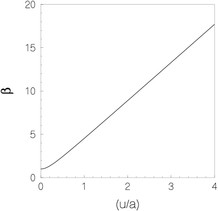
Figure 4: The predicted electron mass enhacemnt $\beta=\tilde{m}/m$ when protons are absorbed into palladium is plotted as a function of the root mean square proton displacement $u$ where $u^{2}=\overline{|{\bf u}|^{2}}$ and the Bohr radius $a\approx 0.5291772108\times 10^{-8}$ cm.

Experimentally[20], for protons absorbed in Pd, one finds the soft Boson mode with $(\hbar\Omega/e)\approx 6\times 10^{-2}\ {\rm volts}$ wherein

$${\cal E}_{\rm p\in Pd}\approx 1.55\times 10^{11}\ {\rm volts/meter}.$$ (87)

In this regard, one notes that typical atomic physics electric fields in atoms are of that order when located a Bohr radius $a$ from an isolated proton; i.e. with the Bohr radius

$$a=\frac{4\pi\hbar^{2}}{e^{2}m}=\frac{\hbar}{\alpha mc}\approx 0.5291772108\times 10^{-8}\ {\rm cm},$$ (88)

atomic electric fields are of the order

$${\cal E}_{a}=\frac{|e|}{4\pi a^{2}}\approx 5.142206318\times 10^{11}\ {\rm volts/meter}.$$ (89)

Employing Eqs.(81), (83) and (89) along with the estimate $\tilde{n}\approx|\psi(0)|^{2}=1/(\pi a^{3})$ yields

$$\frac{\overline{|{\bf E}|^{2}}}{{\cal E}_{a}^{2}}=\frac{16}{9}\left(\frac{\overline{|{\bf u}|^{2}}}{a^{2}}\right).$$ (90)

Thus, Eq.(48) may be written[12] as

$$\beta=\sqrt{\frac{\overline{K^{2}}}{m^{2}c^{4}}}=\sqrt{1+\left[\frac{e^{2}\overline{|{\bf E}|^{2}}}{m^{2}c^{2}\Omega^{2}}\right]}\ ,$$

$$\beta=\frac{\tilde{m}}{m}\approx\sqrt{1+\frac{16{\cal E}_{a}^{2}}{{9{\cal E}}_{\rm p}^{2}}\left(\frac{\overline{|{\bf u}|^{2}}}{a^{2}}\right)}\ .$$ (91)

For example, for protons in palladium Eqs.(87) and (89) imply

$$\beta_{\rm p\in Pd}\approx\sqrt{1+19.6\left(\frac{\overline{|{\bf u}|^{2}}}{a^{2}}\right)},$$ (92)

which is shown in FIG.4.

V.4 Driven Oscillations

When an electrode has a current density passing into the cathode surface, then there is a power per unit area ${\cal P}$ suppled to the surface as in Eq.(3). Under such circumstance the surface temperature rises to a high value. In detail, in a non-equilibrium steady state situation, one must introduce a “noise temperature” $T_{{\bf Q},\omega}$ which depends on the frequency and wave number of the excitations which form due to an Ohmic heating rate per unit time per unit area ${\cal P}={\cal V}{\cal J}$. The noise temperature enters into the dynamic form factor via

$$S(-{\bf Q},-\omega)=e^{-\hbar\omega/k_{B}T_{{\bf Q},\omega}}S({\bf Q},\omega)$$ (93)

which is the non-equilibrium noise temperature version of the thermal equilibrium detailed balance Eq.(74).

Experimentally, the noise temperature is high in the infrared $\omega$-regime in a small surface domain size $d$ related to the wave number via $d\sim Q^{-1}$. Note that the overall temperature over the whole electromagnetic bandwidth need not be very high, but in the infrared regime at $\omega\sim\Omega$ there should be a sharp peak in the noise temperature. What has been observed[27] for deuterons absorbed in palladium, are surface hot spots flashing in different domains analogous to the flashing of fire-flies during a dark evening in the country. The flashing turns on and off in apparently random spatial and temporal patterns. The hot spots occur when and where regions of the rough cathode surface form electromagnetic cavities of size and shape as to naturedly support the infrared radiation. These occur randomly on rough cathode surfaces.

During these flash events the nuclear transmutations can take place. The hot spots at any given time take up only a small fraction of the cathode surface. Increasing the relative fraction of nuclear-active cathode surface area which comprises hot spots would proportionately increase the measured efficiency of neutron production on the cathode. The higher the average density of hot spots on a given cathode surface over time, the greater the amount of excess heat that would likely be observed at the cathode device level using gross thermal measurement techniques such as calorimetry. From the nature of the surface damage on cathodes due to micron-scale hot spots, it is evident that the metal actually melts locally during a hot flash producing nuclear transmutations. Distinctive areas of obvious melting and explosive blow-out cratering features that are consistent with the presence of such hot spots are very commonly seen in post-experiment SEM images of the surfaces of various metallic cathode materials that include gold (melting point $1554.9\ ^{o}C$; boiling point $2963\ ^{o}C$); palladium (melting point $1554.9\ ^{o}C$; boiling point $2963\ ^{o}C$)[28, 29]; titanium (melting point $1064.18\ ^{o}C$; boiling point $2856\ ^{o}C$)[30], and tungsten (melting point $3422\ ^{o}C$; boiling point $5555\ ^{o}C$)[31]. Such evidence is consistent with the noise temperature at a typical value of the peak $T_{{\bf Q},\omega}\sim 5\times 10^{3}\ {}^{o}K$ corresponding to a proton displacement of $(u/a)\sim 10$ within a domain. In accordance with FIG.4, the mass enhancement is more than sufficent for the neutron production Eqs.(1) and (2).

VI Neutrons and Isotopic Spin Waves

The sources of the neutrinos are inhomogeneous in spatial regions near the surfaces of cathodes. Also, the neutrinos are so weakly interacting that after emission they are virtually unaware of the condensed matter. The neutrino on energy shell phase space $Q^{\nu}=({\bf Q},|{\bf Q}|)$ has the Lorentz invariant phase space

$$dL_{\bf Q}=\left[\frac{d^{3}{\bf Q}}{2(2\pi)^{3}|{\bf Q}|}\right].$$ (94)

Writing the neutrino emission part of Eqs.(40) and (41) as the phase space integral

$$\varpi(x)=-c\ {\Im m}\int\int e^{iQ\cdot(x-y)}h^{\lambda\mu\sigma\nu}Q_{\mu}\times$$

$$\left<W^{-}_{\lambda}(x)\bar{\psi}(x)\gamma_{\nu}P_{+}\psi(y)W^{+}_{\sigma}(y)\right>d^{4}ydL_{\bf Q}$$

$$=-4c\left(\frac{\hbar G_{F}}{c^{4}}\right)^{2}\ {\Im m}\int\int e^{iQ\cdot(x-y)}h^{\lambda\mu\sigma\nu}Q_{\mu}\times$$

$$\left<{\cal I}^{-}_{\lambda}(x)\bar{\psi}(x)P_{-}\gamma_{\nu}\psi(y){\cal I}^{+}_{\sigma}(y)\right>d^{4}ydL_{\bf Q}\ .$$ (95)

Under the assumption that the initial proton spins are uncorrelated and that the free neutron density is dilute, considerable simplification can be made in estimating the rather daunting but rigorous Eq.(95). The estimate for the inhomogeneous ultra low momentum neutron production rate per unit volume is

$$\varpi(x)\approx\left(\frac{\hbar G_{F}}{c^{3}}\right)^{2}\left(\frac{2mc^{2}}{\hbar}\right)(g_{V}^{2}+3g_{A}^{2})\times$$

$$\ {\Re e}\int\int e^{iQ\cdot(x-y)}\left<{\cal T}^{+}(x)\bar{\psi}(x)\psi(y){\cal T}^{-}(y)\right>d^{4}ydL_{\bf Q},\$$ (96)

wherein Eq.(19) has been invoked.

If the neutrons are dilute, then it is sufficient to consider the creation of a single neutron from a proton, i.e. the propagation of the $W^{\pm}$ within condensed matter. What is left of the heavy $W^{\pm}$ boson is merely an isotopic spin wave. There is a superposition of amplitudes summed over all the possible protons within a patch which may be converted into a neutron. The isotopic spin wave creation and annihilation operators in the surface patch obey

$${\cal T}^{\pm}(x)\approx{\cal T}^{\pm}({\bf x})e^{\mp i(c\Delta M)x^{0}/\hbar}$$ (97)

with the neutron-proton mass difference determining the threshold value of the electron mass $m$ renormalization parameter $\beta$ i.e.

$$\Delta M=M_{n}-M=\beta_{0}m.$$ (98)

For the creation of a single ultra low momentum neutron from non-relativistic protons

$$\left<{\cal T}^{+}(x)\bar{\psi}(x)\psi(y){\cal T}^{-}(y)\right>\Rightarrow$$

$$\delta({\bf x}-{\bf y})e^{-i(c\Delta M)(x^{0}-y^{0})/\hbar}\times$$

$$\left<p^{\dagger}(x)\bar{\psi}(x)\psi(y)p(y)\right>.$$ (99)

For steady state production rates, Eq.(96) reads

$$\frac{\hbar\varpi({\bf r})}{mc^{2}}\approx 2\left(\frac{\hbar G_{F}}{c^{3}}\right)^{2}(g_{V}^{2}+3g_{A}^{2})\times$$

$$\ {\Re e}\int\int e^{i(c^{2}\Delta M+\hbar c|{\bf Q}|)t/\hbar}\times$$

$$\left<p^{\dagger}({\bf r})\bar{\psi}({\bf r})\psi({\bf r,t})p({\bf r,t})\right>(cdt)dL_{\bf Q}.$$ (100)

Explicitly exhibiting the neutrino energy being radiated away in Eq.(2), yields

$$\frac{\hbar\varpi({\bf r})}{mc^{2}}\approx\frac{1}{2\pi^{2}c^{2}}\left(\frac{\hbar G_{F}}{c^{3}}\right)^{2}(g_{V}^{2}+3g_{A}^{2})\times$$

$$\ {\Re e}\int_{0}^{\infty}\int_{-\infty}^{\infty}e^{i(c^{2}\Delta M+\hbar c|{\bf Q}|)t/\hbar}\times$$

$$\left<p^{\dagger}({\bf r})\bar{\psi}({\bf r})\psi({\bf r,t})p({\bf r,t})\right>(cdt)(\omega d\omega).$$ (101)

The remaining correlation function in Eq.(100) describes how an electron which finds itself directly on top of a proton propagates in time. The integral over time may be written

$${\Re e}\int_{-\infty}^{\infty}\left<p^{\dagger}({\bf r})\bar{\psi}({\bf r})\psi({\bf r,t})p({\bf r,t})\right>e^{iEt/\hbar}dt$$

$$=2\pi\hbar{\cal N}({\bf r})n_{e}({\bf r},E),$$ (102)

wherein ${\cal N}({\bf r})$ is the mean density per unit volume of protons and $n_{e}({\bf r},E)$ is the mean collective density per unit volume per unit energy of electrons which sit directly on the protons.

The steady state inhomogeneous production of neutrons per unit time per unit volume $\varpi({\bf r})$ as estimated in Eq.(101); i.e. exhibiting the radiated neutrino energy $\hbar\omega$,

$$\varpi({\bf r})\approx\frac{mc^{2}}{\pi\hbar}\left(\frac{\hbar G_{F}}{c^{3}}\right)^{2}(g_{V}^{2}+3g_{A}^{2}){\cal N}({\bf r}){\cal K}({\bf r}),$$

$${\cal K}({\bf r})=\frac{\hbar}{c}\int_{0}^{\infty}n_{e}({\bf r},E=c^{2}\Delta M+\hbar\omega)\omega d\omega,$$ (103)

wherein $n_{e}({\bf r},E)$ must be calculated including the surface radiation energy and the driving current through the cathode.

The calculation of ${\cal K}$ depends on the detailed physical properties of the cathode surface as well as the flux $\tilde{\Phi}$ per unit area per unit time of electrons determining the chemical cell current as in the power Eq.(3). In the most simple model, let us consider a smooth surface with material properties and electron currents determining the neutron creation rate via the mass renormalization parameter $\beta$ as defined in Eq.(48). We note in passing that a smooth surface is not likely to be the best surface for producing neutrons since rough surfaces have patches wherein the surface plasma electromagnetic field oscillations will be very much more intense. However, the following smooth surface model will be employed for estimating the proper low energy nuclear reaction rates produced by electroweak interactions.

To compute the density of surface electron states per unit area per unit energy, one may begin with a simple renormalized electron mass $\tilde{m}$ model and take

$$g_{2}(E)=2\int\delta\left(E-\sqrt{c^{2}p^{2}+(\tilde{m}c^{2})^{2}}\right)\frac{d^{2}{\bf p}}{(2\pi\hbar)^{2}}\ ,$$ (104)

i.e.

$$g_{2}(E)=\frac{E}{\pi\hbar^{2}c^{2}}\ .$$ (105)

If such surface electron states are confined to a wave function width $l$ normal to the surface, then we have within the surface region, and after integrating over the emitted neutrino energy spectrum

$${\cal K}\approx\frac{\hbar}{lc}\int g_{2}(E=\beta_{0}mc^{2}+\hbar\omega)\omega d\omega,$$

$${\cal K}\approx\frac{1}{2\pi l}\left(\frac{mc}{\hbar}\right)^{3}(\beta-\beta_{0})^{2}.$$ (106)

For a smooth surface, integrating the neutrino production rate over a thin slab at the electrode surface yields the estimate for the production rate per unit time per unit area,

$$\varpi_{2}\approx\left(\frac{g_{V}^{2}+3g_{A}^{2}}{2\pi^{2}}\right)n_{2}\left(\frac{G_{F}m^{2}}{\hbar c}\right)^{2}\frac{mc^{2}}{\hbar}(\beta-\beta_{0})^{2}.$$ (107)

The above Eq.(107) for smooth surfaces is in agreement with the initial order of magnitude estimate in Eqs.(9) and (10).

VII Conclusions

Electromagnetic surface plasma oscillation energies in hydrogen-loaded metal cathodes may be combined with the normal electron-proton rest mass energies to allow for neutron producing low energy nuclear reactions Eq.(2). The entire process of neutron production near metallic hydride surfaces may be understood in terms of the standard model for electroweak interactions. The produced neutrons have ultra low momentum since the wavelength is that of a low mode isotopic spin wave spanning a surface patch. The radiation energy required for such ultra low momentum neutron production may be supplied by the applied voltage required to push a strong charged current across the metallic hydride cathode surface. Alternatively, low energy nuclear reactions may be induced directly by laser radiation energy applied to a cathode surface. They may even be induced, albeit at comparatively low rates of reaction, simply by imposing an adequate pressure gradient (which can be as little as one atmosphere.) of gaseous hydrogen isotopes across a metallic membrane[32, 33] composed of an aggressive hydride-former such as palladium.

The electroweak rates of the resulting ultra low momentum neutron production are computed from the above considerations. In terms of the radiation induced mass renormalization parameter $\beta$ in Eqs.(7) and (8), the predicted neutron production rates per unit area per unit time have the form

$$\varpi_{2}=\nu(\beta-\beta_{0})^{2}\ \ \ {\rm above\ threshold}\ \ \ \beta>\beta_{0}.$$ (108)

The expected range of the parameter $\nu$ for hydrogen-loaded cathodes is approximately

$$10^{12}\ \frac{\rm Hz}{\rm cm^{2}}\ <\ \nu\ <10^{14}\ \frac{\rm Hz}{\rm cm^{2}}$$ (109)

in satisfactory agreement with the orders of magnitude observed experimentally. More precise theoretical estimates of $\nu$ require specific material science information about the physical state of cathode surfaces which must then be studied in detail. As discussed in previous work[12], a deuteron on certain cathode surfaces may also capture an electron producing two ultra low momentum neutrons and a neutrino. The neutron production rates for heavy water systems are thereby somewhat enhanced.

From a technological perspective, we note that energy must first be put into a given metallic hydride system in order to renormalize electron masses and reach the critical threshold values at which neutron production can occur. Net excess energy, actually released and observed at the physical device level, is the result of a complex interplay between the percentage of total surface area having micron-scale E and B field strengths high enough to create neutrons and elemental isotopic composition of near-surface target nuclei exposed to local fluxes of readily captured ultra low momentum neutrons. In many respects, low temperature and pressure low energy nuclear reactions in condensed matter systems resemble r- and s-process nucleosynthetic reactions in stars. Lastly, successful fabrication and operation of long lasting energy producing devices with high percentages of nuclear active surface areas will require nanoscale control over surface composition, geometry and local field strengths.

References

- [1] Y. Iwamura, T. Itoh, N. Gotoh, and I. Toyoda, Fusion Tech. 33, 476 (1998).
- [2] V. Violante, E. Castagna, C. Sibilia, S. Paoloni, and F. Sarto, Analysis of Ni-Hydride Thin Film after Surface Plasmon Generation by Laser Technique, Condensed Matter Nuclear Science, Proceedings of ICCF-10, P. Hagelstein and S. Chubb, Eds. World Scientific Publishing, Singapore, 421 (2002).
- [3] J. Dash and D. Chicea, Changes in the Radioactivity, Topography, and Surface Composition of Uranium after Hydrogen Loading by Aqueous Electrolysis, Condensed Matter Nuclear Science, Proceedings of ICCF-10, P. Hagelstein and S. Chubb, Eds., World Scientific Publishing, Singapore, 463 (2002).
- [4] G.H. Miley, G. Narne, and T. Woo, J. Rad. Nuc. Chem. 263, 691 (2005).
- [5] G.H. Miley and J. A. Patterson, J. New Energy 1, 11 (1996).
- [6] G.H. Miley, J. New Energy 2, 6 (1997).
- [7] S. Pons in News, Nature 338, 681 (1989).
- [8] R.E. Marshak, Riazuddin and C.P. Ryan, Theory of Weak Interaction of Elementary Particles, Interscience, New York (1969).
- [9] S. Pokorski, Gauge Field Theories, second edition, Cambridge University Press, Cambridge (2000).
- [10] T. Mizuno, Nuclear Transmutation: The Reality of Cold Fusion, Infinite Energy Press, Concord (1998).
- [11] H. Kozima, Discovery of the Cold Fusion Phenomenon, Ohotake Shuppan, Tokyo (1998).
- [12] A. Widom and L. Larsen Eur. Phys. J. C 46, 107 (2006).
- [13] A. Widom and L. Larsen, arXiv:cond-mat/0509269v1, 10 Sep 2005.
- [14] B. Cassin and E.U. Condon, Phys. Rev. 50, 846 (1936).
- [15] G. Gamow and E. Teller, Phys. Rev. 48, 895 (1936).
- [16] V.B. Berestetskii, E.M. Lifshitz and L.P. Pitaevskii, Quantum Electrodynamics, Sec.40, Eq.(40.15), Butterworth Heinmann, Oxzford (1997).
- [17] L.D. Landau and E.M. Lifshitz, The Classical Theory of Fields, Secs.17 and 47 Prob.2, Pergamon Press, Oxford (1975).
- [18] C. A. Chatzidimitriou-Dreismann, T. Abdul-Redah, and M. Krzystyniak1, Phys. Rev. B 72, 054123 (2005).
- [19] R A. Cowley and J Mayers, Phys.: Condens. Matter 18, 5291 (2006).
- [20] M. Kemali, J. E. Totolici, D. K. Ross, and I. Morrison, Phys. Rev. Lett. 84, 1531 (2000);
- [21] A.I. Kolesnikova, V.E. Antonovb, V.K. Fedotova, G. Grossec, A.S. Ivanovd and F.E. Wagner, Physica B, 158 (2002).
- [22] I.Y. Glagolenko1, K.P. Carney1, S. Kern, E.A. Goremychkin, T.J.Udovic, J.R.D. Copley, J.C. Cook, Appl. Phys. A 74, S1397 (2002).
- [23] Nikitas I. Gidopoulos, Phys. Rev. B 71, 054106 (2005).
- [24] D. Medini and A. Widom, J. Chem. Phys. 118 2405 (2003). J. Phys.: Condens. Matter 18 5291 (2006).
- [25] M. Krzystyniak and C.A. Chatzidimitriou-Dreismann, Journal of Neutron Research, 14, 193 (2006).
- [26] G. F. Reiter and P. M. Platzman, Phys. Rev. B 71, 054107 (2004).
- [27] S. Szpak, P.A. Mosier-Boss, J. Dea, and F. Gordon, International Conference on Cold Fusion, World Scientific Inc. (2003).
- [28] Y. Toriyabe, T. Mizuno, T. Ohmori, and Y. Aoki, Elemental Analysis of Palladium Electrodes After Pd/Pd Light Water Critical Electrolysis, Eds. A. Takahashi, K. Ota, and Y. Iwamura, Proceedings of ICCF-12, page 252, World Scientific Publishing, Singapore (2006).
- [29] S. Szpak, P. Boss, C. Young, and F. Gordon, Naturwissenschaften 92, 394 (2005).
- [30] I. Savvatimova and D. Gavritenkov, Results of Analysis of Ti Foil After Glow Discharge with Deuterium, Proceedings of ICCF-11, Ed. J. Biberian, page 438, World Scientific Publishing, Singapore, (2006).
- [31] D. Cirillo, and V. Iorio, Transmutation of Metal at Low Energy in a Confined Plasma in Water, Ed. J. Biberian, page 492, Proceedings of ICCF-11, World Scientific Publishing, Singapore, (2006).
- [32] Y. Iwamura, M. Sakano and T. Itoh, Jpn. J. Appl. Phys. 41, 4642 (2002).
- [33] X. Li, B. Liu, J. Tian, Q. Wei, R. Zhou and Z. Yu, J. Phys. D: Appl. Phys., 36, 3095 (2003).