A FAST HADRON FREEZE-OUT GENERATOR

Abstract

We have developed a fast Monte Carlo procedure of hadron generation allowing one to study and analyze various observables for stable hadrons and hadron resonances produced in ultra-relativistic heavy ion collisions. Particle multiplicities are determined based on the concept of chemical freeze-out. Particles can be generated on the chemical or thermal freeze-out hypersurface represented by a parameterization or a numerical solution of relativistic hydrodynamics with given initial conditions and equation of state. Besides standard space-like sectors associated with the volume decay, the hypersurface may also include non-space-like sectors related to the emission from the surface of expanding system. For comparison with other models and experimental data we demonstrate the results based on the standard parameterizations of the hadron freeze-out hypersurface and flow velocity profile under the assumption of a common chemical and thermal freeze-out. The C++ generator code is written under the ROOT framework and is available for public use at http://uhkm.jinr.ru/.

I Introduction

Ongoing and planned experimental studies of relativistic heavy ion collisions in a wide range of beam energies require a development of new event generators and improvement of the existing ones Heavy_Ions . Especially for Large Hadron Collider (LHC) experiments, because of very high hadron multiplicities, one needs fairly fast Monte-Carlo (MC) generators for event simulation.

A successful but oversimplified attempt of creating a fast hadron generator motivated by hydrodynamics was done in Ref. Snigiriev96 ; Kruglov97 ; Lokhtin03 ; Lokhtin05 . The present work is an extension of this approach. We formulate a fast MC procedure to generate hadron multiplicities, four-momenta and four-coordinates for any kind of freeze-out hypersurface. Decays of hadronic resonances are taken into account. We consider hadrons consisting of light $u$,$d$ and $s$ quarks only, but the extension to heavier quarks is possible. The generator code is written in the object-oriented C++ language under the ROOT framework ROOT .

In this article we discuss only central collisions of nuclei using the Bjorken-like and Hubble-like freeze-out parameterizations used in so-called ”blast wave” Lisa and ”Cracow” models Bron04 , respectively. The same parametrizations have been used in the hadron generator referred as THERMINATOR THERMINATOR that appears however less efficient than our generator (see sections II, VI).

The paper is now organized as follows. Sections  II-V are devoted to the description of the physical framework of the model. In section VI, the Monte Carlo simulation procedure is formulated. The validation of this procedure is presented in section VII. In section VIII, the example calculations are compared with the Relativistic Heavy Ion Collider (RHIC) experimental data. We summarize and conclude in section IX.

II Hadron multiplicities

We give here the basic formulae for the calculation of particle multiplicities. We consider the hadronic matter created in heavy-ion collisions as a hydrodynamically expanding fireball with the equation of state of an ideal hadron gas.

The mean number $\bar{N}_{i}$ of particles species $i$ crossing the space-like freeze-out hypersurface $\sigma(x)$ in Minkowski space can be computed as RKT

$$\bar{N}_{i}=\int_{\sigma(x)}d^{3}\sigma_{\mu}(x)j^{\mu}_{i}(x).$$ (1)

Here the four-vector $d^{3}\sigma_{\mu}(x)=n_{\mu}(x)d^{3}\sigma(x)$ is the element of the freeze-out hypersurface directed along the hypersurface normal unit four-vector $n^{\mu}(x)$ with a positively defined zero component ($n^{0}(x)>0$) and $d^{3}\sigma(x)=|d^{3}\sigma_{\mu}d^{3}\sigma^{\mu}|^{1/2}$ is the invariant measure of this element. The normal to the space-like hypersurface is time-like, i.e. $n^{\mu}n_{\mu}=1$; generally, for hypersurfaces including non-space-like sectors, the normal can also be a space-like so then $n^{\mu}n_{\mu}=-1$. The four-vector $j^{\mu}_{i}(x)$ is the current of particle species $i$ determined as:

$$j^{\mu}_{i}(x)=\int\frac{d^{3}\vec{p}}{p^{0}}p^{\mu}f_{i}(x,p),$$ (2)

where $f_{i}(x,p)$ is the Lorentz invariant distribution function of particle freeze-out four-coordinate $x=\{x^{0},\vec{x}\}$ and four-momentum $p=\{p^{0},\vec{p}\}$. In the case of local equilibrium

$$f_{i}(x,p)=f_{i}^{{\rm eq}}(p\cdot u(x);T(x),\mu(x))=\frac{1}{(2\pi)^{3}}\frac{g_{i}}{\exp{([p\cdot u(x)-\mu_{i}(x)]/T(x))}\pm 1},$$ (3)

where $p\cdot u\equiv p^{\mu}u_{\mu}$, $g_{i}=2J_{i}+1$ is the spin degeneracy factor, $T(x)$ and $\mu_{i}(x)$ are the local temperature and chemical potential respectively, $u(x)=\gamma\{1,\vec{v}\}$ is the local collective four-velocity, $\gamma=(1-v^{2})^{-1/2}$, $u^{\mu}u_{\mu}=1$. The signs $\pm$ in the denominator account for the proper quantum statistics of a fermion or a boson, respectively.

The Lorentz scalar local particle density is defined as:

$$\rho_{i}(x)=u_{\mu}(x)j^{\mu}_{i}(x)=\int\frac{d^{3}\vec{p}}{p^{0}}p_{\mu}u^{\mu}(x)f_{i}(x,p).$$ (4)

For a system in local thermal equilibrium, the particle density in the fluid element rest frame, where $u^{*\mu}=\{1,0,0,0\}$, is solely determined by the local temperature $T(x^{*})$ and chemical potential $\mu_{i}(x^{*})$ for each particle species $i$:

$$\rho_{i}^{\rm eq}(T(x^{*}),\mu_{i}(x^{*}))=u_{\mu}^{*}j^{{\rm eq}\mu}_{i}(x^{*})=\int d^{3}\vec{p}^{~{}*}f_{i}^{\rm eq}(p^{*0};T(x^{*}),\mu_{i}(x^{*}));$$ (5)

the four-vectors in fluid element rest frames are denoted by star.

In the case of local equilibrium, the particle current is proportional to the fluid element four-velocity: $j^{{\rm eq}\mu}_{i}(x)=\rho_{i}^{\rm eq}(T(x),\mu_{i}(x))u^{\mu}(x)$. So the mean number of particles of species $i$ is expressed directly through the equilibrated density:

$$\bar{N}_{i}=\int_{\sigma(x)}d^{3}\sigma_{\mu}(x)u^{\mu}(x)\rho_{i}^{\rm eq}(T(x),\mu_{i}(x)).$$ (6)

In the case of constant temperature and chemical potential, $T(x)=T$ and $\mu_{i}(x)=\mu_{i}$, one has

$$\bar{N}_{i}=\rho_{i}^{\rm eq}(T,\mu_{i})\int_{\sigma(x)}d^{3}\sigma_{\mu}(x)u^{\mu}(x)=\rho_{i}^{\rm eq}(T,\mu_{i})V_{\rm eff},$$ (7)

i.e. the total yield of particle species $i$ is determined by the freeze-out temperature $T$, chemical potential $\mu_{i}$ and by the total co-moving volume $V_{\rm eff}$, so called effective volume of particle production which is a functional of the field of collective velocities $u^{\mu}(x)$ on the hypersurface $\sigma(x)$. The effective volume absorbs the collective velocity profile and the form of hypersurface and cancels out in all particle number ratios. Therefore, the particle number ratios do not depend on the freeze-out details as long as the local thermodynamic parameters are independent of $x$. The concept of the effective volume and factorization property similar to Eq. (7) has been considered first in Ref. Nukleonika , repeatedly used for the analysis of particle number ratios (see, e.g., Ref. Sinyukov02 ) and recently generalized for a study of the averaged phase space densities AkkSin1 and entropy AkkSin2 . One can apply this concept also in a limited rapidity window Nukleonika ; AkkSin1 ; AkkSin2 .

The concept of the effective volume can be applied to calculate the hadronic composition at both chemical and thermal freeze-outs Sinyukov02 . At the former one, which happens soon after hadronization, the chemically equilibrated hadronic composition is assumed to be established and frozen in further evolution. The chemical potential $\mu_{i}$ for any particle species $i$ at the chemical freeze-out is entirely determined by chemical potentials $\widetilde{\mu_{q}}$ per a unit charge, i.e. per unit baryon number $B$, strangeness $S$, electric charge $Q$, charm $C$, etc. It can be expressed as a scalar product:

$$\mu_{i}=\vec{q}_{i}\vec{\widetilde{\mu}},$$ (8)

where $\vec{q}_{i}=\{B_{i},S_{i},Q_{i},C_{i},...\}$ and $\vec{\widetilde{\mu}}=\{\widetilde{\mu}_{B},\widetilde{\mu}_{S},\widetilde{\mu}_{Q},\widetilde{\mu}_{C},..\}$. Assuming constant temperature and chemical potentials on the chemical freeze-out hypersurface, the total quantum numbers $\vec{q}=\{B,S,Q,C,...\}$ of the selected thermal part of produced hadronic system (e.g., in a rapidity interval near $y=0$) with corresponding $V_{\rm eff}$ can be calculated as $\vec{q}=V_{\rm eff}\sum_{i}\rho_{i}^{\rm eq}\vec{q}_{i}$. For example:

$$B=V_{\rm eff}\sum_{i=1}^{n}\rho_{i}^{\rm eq}(T,\mu_{i})B_{i},$$ (9)

$$S=V_{\rm eff}\sum_{i=1}^{n}\rho_{i}^{\rm eq}(T,\mu_{i})S_{i},$$ (10)

$$Q=V_{\rm eff}\sum_{i=1}^{n}\rho_{i}^{\rm eq}(T,\mu_{i})Q_{i}.$$ (11)

The potentials $\widetilde{\mu}_{q}$ are not independent. Thus, taking into account baryon, strangeness and electrical charges only and fixing the total strangeness $S$ and the total electric charge $Q$, $\widetilde{\mu}_{S}$ and $\widetilde{\mu}_{Q}$ can be expressed through baryonic potential $\widetilde{\mu}_{B}$ using Eqs. (10) and (11). Therefore the mean numbers of each particle and resonance species at chemical freeze-out are determined solely by the temperature $T$ and baryonic chemical potential $\widetilde{\mu}_{B}$.

In practical calculations, we use the phenomenological observation Cleymans05 that particle yields in central Au+Au or Pb+Pb collisions in a wide center-of-mass energy range $\sqrt{s}_{NN}=2.2-200$ GeV can be described within the thermal statistical approach using the following parametrizations of the temperature and baryon chemical potential Cleymans05 :

$$T(\widetilde{\mu}_{B})=a-b\widetilde{\mu}^{2}_{B}-c\widetilde{\mu}^{4}_{B},$$ (12)

$$\widetilde{\mu}_{B}(\sqrt{s}_{NN})=\frac{d}{1+e\sqrt{s}_{NN}},$$ (13)

$a=0.166\pm 0.002$ GeV, $b=0.139\pm 0.016$ GeV^-1, $c=0.053\pm 0.021$ GeV^-3 and $d=1.308\pm 0.028$ GeV, $e=0.273\pm 0.008$ GeV^-1.

The particle densities at the chemical freeze-out stage are too high (see, e.g., Sinyukov02 ) to consider particles as free streaming and associate this stage with the thermal freeze-out one. The mean particle numbers $\bar{N}_{i}^{\rm th}$ at thermal freeze-out can be determined using the following procedure Sinyukov02 . First, the temperature and chemical potentials at chemical freeze-out have to be fitted from the ratios of the numbers of (quasi)stable particles. The fitting procedure should account for the decays of all resonances as well as unstable particles in given experimental conditions (feed-down). The common factor, $V_{\rm eff}^{\rm ch}$, and, thus, the absolute particle and resonance numbers can be fixed, e.g., from pion multiplicities. Within the concept of chemically frozen evolution these numbers are assumed to be conserved except for corrections due to decay of some part of short-lived resonances that can be estimated from the assumed chemical to thermal freeze-out evolution time. Then one can calculate the mean numbers of different particles and resonances reaching a (common) thermal freeze-out hypersurface. At a given thermal freeze-out temperature $T_{\rm th}$ these mean numbers can be expressed through the thermal effective volume $V_{\rm eff}^{\rm th}$ and the chemical potentials for each particle species $\mu^{{\rm th}}_{i}$ which can no more be expressed in the form $\mu_{i}=\vec{q}_{i}\vec{\widetilde{\mu}}$ valid only for chemically equilibrated systems. For a given parametrization of the thermal freeze-out hypersurface, the thermal effective volume $V_{\rm eff}^{\rm th}$ (and thus all $\mu^{{\rm th}}_{i}$) can be fixed with the help of pion interferometry data.

In practical calculations we determine all macroscopic characteristics of a particle system with the temperature $T$ and chemical potentials $\mu_{i}$ via a set of equilibrium distribution functions in the fluid element rest frame:

$$f_{i}^{\rm eq}(p^{*0};T,\mu_{i})=\frac{1}{(2\pi)^{3}}\frac{g_{i}}{\exp{([p^{*0}-\mu_{i}]/T)}\pm 1}.$$ (14)

Eq. $(\ref{M6})$ for the particle number density then reduces to

$$\rho_{i}^{\rm eq}(T,\mu_{i})=4\pi\int_{0}^{\infty}{dp^{*}p^{*2}f_{i}^{\rm eq}(p^{*0};T,\mu_{i})}.$$ (15)

Using the expansion

$$f_{i}^{\rm eq}(p^{*0};T,\mu_{i})=\frac{g_{i}}{(2\pi)^{3}}\sum_{k=1}^{\infty}(\mp)^{k+1}\exp(k\frac{\mu_{i}-p^{*0}_{i}}{T}),$$ (16)

the density can be represented in a form of a fast converging series:

$$\rho_{i}^{\rm eq}(T,\mu_{i})=\frac{g_{i}}{2\pi^{2}}m^{2}_{i}T\sum_{k=1}^{\infty}\frac{(\mp)^{k+1}}{k}\exp(\frac{k\mu_{i}}{T})K_{2}(\frac{km_{i}}{T}),$$ (17)

where $K_{2}$ is the modified Bessel function of the second order.

We assume that the calculated mean particle numbers $\bar{N}_{i}=\rho_{i}^{\rm eq}V_{\rm eff}$ correspond to a grand canonical ensemble. The probability that the ensemble consists of $N_{i}$ particles is thus given by Poisson distribution:

$$P(N_{i})=\exp{(-\bar{N}_{i})}\frac{(\bar{N}_{i})^{N_{i}}}{N_{i}!}.$$ (18)

III Hadron momentum distributions

We suppose that a hydrodynamic expansion of the fireball ends by a sudden system breakup at given temperature and chemical potentials. In this case the momentum distribution of the produced hadrons keeps the thermal character of the equilibrium distribution $(\ref{M2P})$. Similar to Eqs. (1), (2), this distribution is then calculated according to the Cooper-Frye formula Cooper74 :

$$p^{0}\frac{d^{3}\bar{N}_{i}}{d^{3}p}=\int_{\sigma(x)}d^{3}\sigma_{\mu}(x)p^{\mu}f^{\rm eq}_{i}(p\cdot u(x);T,\mu_{i}).$$ (19)

The integral in Eq. (19) can be calculated with the help of the invariant weight

$$W_{\sigma,i}(x,p)\equiv p^{0}\frac{d^{6}\bar{N}_{i}}{d^{3}\sigma d^{3}\vec{p}}=n_{\mu}(x)p^{\mu}f_{i}^{\rm eq}(p\cdot u(x);T,\mu_{i}).$$ (20)

It is convenient to transform the four-vectors into the fluid element rest frame, e.g.,

$$\begin{array}[]{c}n^{*0}=n^{\mu}u_{\mu}=\gamma(n^{0}-\vec{v}\vec{n}),\\ \vec{n}^{*}=\vec{n}-\gamma(1+\gamma)^{-1}(n^{*0}+n^{0})\vec{v}\end{array}$$ (21)

and calculate the weight in this frame:

$$W_{\sigma,i}(x,p)=W_{\sigma,i}^{*}(x^{*},p^{*})=n_{\mu}^{*}(x)p^{*\mu}f_{i}^{\rm eq}(p^{*0};T,\mu_{i}).$$ (22)

Particulary, in the case when the normal four-vector $n^{\mu}(x)$ coincides with the fluid element flow velocity $u^{\mu}(x)$, i.e. $n^{*\mu}=u^{*\mu}=\{1,0,0,0\}$, the weight $W_{\sigma,i}^{*}(x^{*},p^{*})=p^{*0}f_{i}^{\rm eq}(p^{*0};T,\mu)$ is independent of $x$ and isotropic in the three-momentum ${\vec{p}}^{~{}*}$. A simple and $100\%$ efficient simulation procedure can then be realized in this frame and the four-momenta of the generated particles transformed back to the fireball rest frame using the velocity field $\vec{v}(x)$:

$$\begin{array}[]{c}p^{0}=\gamma(p^{0*}+\vec{v}\vec{p}^{~{}*}),\\ \vec{p}=\vec{p}^{~{}*}+\gamma(1+\gamma)^{-1}(p^{0*}+p^{0})\vec{v}.\end{array}$$ (23)

There are two well-known examples of the models giving $n^{\mu}(x)=u^{\mu}(x)$: the Bjorken model with hypersurface $\tau_{B}=(t^{2}-z^{2})^{1/2}=const$ and absent transverse flow and the model with hypersurface $\tau_{H}=(t^{2}-x^{2}-y^{2}-z^{2})^{1/2}=const$ and spherically symmetric Hubble flow. In general case $n_{\mu}(x)$ may differ from $u_{\mu}(x)$ and one should account for the $x-p$ correlation and the corresponding anisotropy due to the factor $n_{\mu}p^{\mu}$ even in the fluid element rest frame GorSin .

IV Generalization of the Cooper-Frye prescription

It is well known that the Cooper-Frye freeze-out prescription in Eq. (19) is not valid for the part of the freeze-out hypersurface characterized by a space-like normal four-vector $n^{\mu}$. In this case $|n^{0}|<|\vec{n}|$ and so $p^{\mu}n_{\mu}<0$ for some particle momenta thus leading to negative contributions to particle numbers. Usually, the negative contributions are simply rejected Sin4 ; Bugaev . This procedure however violates the continuity condition of the flow $\rho_{i}u^{\mu}n_{\mu}$ through the freeze-out hypersurface. Taking into account the continuity of the particle flow, the generalization of Eq. (19) has the form Sin4 :

$$p^{0}\frac{d^{3}\bar{N}_{i}}{d^{3}p}=\int_{\sigma(x)}d^{3}\sigma_{\mu}(x)\pi^{\mu}(x,p)f_{i}^{\rm eq}(T(x),\mu_{i}(x)),$$ (24)

where

$$\begin{array}[]{c}\pi^{\mu}(x,p)=p^{\mu}\theta(1-|\widetilde{\lambda}(x,p)|)+u^{\mu}(x)~{}p\cdot u(x)~{}\theta(|\widetilde{\lambda}(x,p)|-1),\\ \widetilde{\lambda}(x,p)=1-{p\cdot n(x)}~{}[{p\cdot u(x)~{}n(x)\cdot u(x)}]^{-1},\end{array}$$ (25)

$\theta(x)=1$ for $x\geq 0$, $\theta(x)=0$ for $x<0$.

Passing to the fluid element rest frames at each point $x$ and using Lorentz transformation properties of the quantities in Eq. (24), one arrives at the same form of the four-vector of particle flow as in the case of the freeze-out hypersurface with the time-like normal $n^{\mu}(x)$:

$$j^{\mu}(x)=\int\frac{d^{3}\vec{p}}{p_{0}}\pi^{\mu}(x,p)f_{i}^{\rm eq}(T(x),\mu_{i}(x))=\rho_{i}^{\rm eq}(T(x),\mu_{i}(x))u^{\mu}(x).$$ (26)

Therefore the factorization of the freeze-out details in the effective volume in the case of constant temperature and chemical potentials, i.e. Eq. (7), is valid for any type of hypersurface AkkSin1 . It follows from Eqs. (24), (25) that the invariant weight in the fluid element rest frame has then the form:

$$W^{*}_{\sigma,i}(x^{*},p^{*})=\left[p^{*\mu}n_{\mu}^{*}~{}\theta\left(1-\left|\frac{\vec{p}^{~{}*}\vec{n}^{~{}*}}{p^{*0}n^{*0}}\right|\right)+p^{*0}n^{*0}~{}\theta\left(\left|\frac{\vec{p}^{~{}*}\vec{n}^{~{}*}}{p^{*0}n^{*0}}\right|-1\right)\right]f_{i}^{\rm eq}(p^{*0};T,\mu_{i}).$$ (27)

For the time-like normal $n^{\mu}(x)$, Eq. (27) reduces to Eq. (22).

It is worth noting that though the bulk of particles is likely associated with the volume decay, the particle emission from the surface of expanding system, or formally, from a non-space-like part of the freeze-out hypersurface enclosed in Minkowski space, is essential for a description of hadronic spectra and like pion correlations at relatively large $p_{T}$ Borysova .

V Freeze-out surface parameterizations

In principle, one can specify the fireball initial conditions (e.g., Landau- or Bjorken-like) and equation of state to follow the fireball dynamic evolution until the freeze-out stage with the help of relativistic hydrodynamics. The corresponding freeze-out four-coordinates $x^{\mu}$, the hypersurface normal four-vectors $n^{\mu}(x)$ and the collective flow four-velocities $u^{\mu}(x)$ can then be used to calculate particle spectra according to generalized Cooper-Frye prescription. This possibility is forseen as an option in our MC generator. In this paper, we however do not consider the fireball evolution, we demonstrate our fast MC procedure utilizing the simple and frequently used parametrizations of the freeze-out.

At relativistic energies, due to dominant longitudinal motion, it is convenient to substitute the Cartesian coordinates $t$, $z$ by the Bjorken ones

$$\tau=(t^{2}-z^{2})^{1/2},~{}~{}\eta=\frac{1}{2}\ln\frac{t+z}{t-z}$$ (28)

and introduce the the radial vector $\vec{r}\equiv\{x,y\}=\{r\cos\phi,r\sin\phi\}$, i.e.:

$$x^{\mu}=\{\tau\cosh\eta,\vec{r},\tau\sinh\eta\}=\{\tau\cosh\eta,r\cos\phi,r\sin\phi,\tau\sinh\eta\}.$$ (29)

Similarly, it is convenient to parameterize the fluid flow four-velocity $u^{\mu}(x)=\gamma(x)\{1,\vec{v}(x)\}\equiv\gamma(x)\{1,\vec{v}_{r}(x),v_{z}(x)\}$ at a point $x$ in terms of the longitudinal ($z$) and transverse ($r$) fluid flow rapidities

$$\eta_{u}(x)=\frac{1}{2}\ln{\frac{1+v_{z}(x)}{1-v_{z}(x)}},~{}~{}\rho_{u}(x)=\frac{1}{2}\ln{\frac{1+v_{r}(x)\cosh\eta_{u}(x)}{1-v_{r}(x)\cosh\eta_{u}(x)}},$$ (30)

where $v_{r}=|\vec{v}_{r}|$ is the magnitude of the transverse component of the flow three-velocity $\vec{v}=\{v_{r}\cos\phi_{u},v_{r}\sin\phi_{u},v_{z}\}$, i.e.

$$\begin{array}[]{c}u^{\mu}(x)=\{\cosh\rho_{u}\cosh\eta_{u},\sinh\rho_{u}\cos\phi_{u},\sinh\rho_{u}\sin\phi_{u},\cosh\rho_{u}\sinh\eta_{u}\}\\ =\{(1+u_{r}^{2})^{1/2}\cosh\eta_{u},\vec{u}_{r},(1+u_{r}^{2})^{1/2}\sinh\eta_{u}\},\end{array}$$ (31)

$\vec{u}_{r}=\gamma\vec{v}_{r}=\gamma_{r}\cosh\eta_{u}\vec{v}_{r}$, $\gamma_{r}=\cosh\rho_{u}$. For the considered central collisions of symmetric nuclei, $\phi_{u}=\phi$. Representing the freeze-out hypersurface by the equation $\tau=\tau(\eta,r,\phi),$ the hypersurface element in terms of the coordinates $\eta$, $r$, $\phi$ becomes

$$d^{3}\sigma_{\mu}=\epsilon_{\mu\alpha\beta\gamma}\frac{dx^{\alpha}dx^{\beta}dx^{\gamma}}{d\eta drd\phi}d\eta drd\phi,$$ (32)

where $\epsilon_{\mu\alpha\beta\gamma}$ is the completely antisymmetric Levy-Civita tensor in four dimensions with $\epsilon^{0123}=-\epsilon_{0123}=1$. Particulary, for azimuthaly symmetric hypersurface $\tau=\tau(\eta,r)$, Eq. (32) yields Sinyukov02 :

$$d^{3}\sigma_{\mu}=\tau(\vec{r},\eta)d^{2}\vec{r}d\eta\{\frac{1}{\tau}\frac{d\tau}{d\eta}\sinh\eta+\cosh\eta,-\frac{d\tau}{dr}\cos\phi,-\frac{d\tau}{dr}\sin\phi,-\frac{1}{\tau}\frac{d\tau}{d\eta}\cosh\eta-\sinh\eta\}.$$ (33)

Generally, the freeze-out hypersurface is represented by a set of equations $\tau=\tau_{j}(\eta,r,\phi)$ and Eq. (32) should be substituted by the sum of the corresponding hypersurface elements.

To simplify the situation, besides the azimuthal symmetry, we further assume the longitudinal boost invariance Bjorken83 . The local quantities (such as particle density) are then functions of $\tau$ and ${r}$ only. The hypersurface then takes the form $\tau=\tau(r)$, the flow rapidities $\eta_{u}=\eta$ (i.e. $v_{z}=z/t$), $\rho_{u}=\rho_{u}(r)$ and Eq. (33) yields

$$\begin{array}[]{c}d^{3}\sigma_{\mu}=\tau(r)d^{2}\vec{r}d\eta\{\cosh\eta,-\frac{d\tau}{dr}\cos\phi,-\frac{d\tau}{dr}\sin\phi,-\sinh\eta\},\cr d^{3}\sigma=|1-(\frac{d\tau}{dr})^{2}|^{1/2}\tau(r)d^{2}\vec{r}d\eta,\cr n^{\mu}(x)=|1-(\frac{d\tau}{dr})^{2}|^{-1/2}\{\cosh\eta,\frac{d\tau}{dr}\cos\phi,\frac{d\tau}{dr}\sin\phi,\sinh\eta\}.\end{array}$$ (34)

Note that the normal four-vector $n^{\mu}$ becomes space-like $(n^{\mu}n_{\mu}=-1)$ for $|d\tau/dr|>1$.

For the simplest freeze-out hypersurface $\tau=const$ one has

$$\begin{array}[]{c}d^{3}\sigma=\tau d^{2}\vec{r}d\eta,\\ n^{\mu}(x)=\{\cosh\eta,0,0,\sinh\eta\}.\end{array}$$ (35)

In this case the normal $n^{\mu}(x)$ is time-like ($n^{\mu}n_{\mu}=1$) but generally different from the flow four-velocity $u^{\mu}(x)$ except for the case of absent transverse flow (i.e. $\rho_{u}=0$). Assuming $\phi_{u}=\phi$ and the linear transverse flow rapidity profile (effectively taking into account a positive flow - radius correlation up to the radii close to the fireball boundary as indicated by numerical solutions of (3+1)-dimensional relativistic hydrodynamics, see, e.g., mor02 ):

$$\rho_{u}=\frac{r}{R}\rho_{u}^{\max},$$ (36)

where $R$ is the fireball transverse radius, the total effective volume for particle production at $\tau=const$ is

$$V_{\rm eff}=\int_{\sigma(x)}d^{3}\sigma_{\mu}(x)u^{\mu}(x)=\tau\int_{0}^{R}\gamma_{r}rdr\int_{0}^{2\pi}d\phi\int_{\eta_{\min}}^{\eta_{\max}}d\eta=$$

$$=2\pi\tau\Delta\eta\left({R\over\rho_{u}^{\max}}\right)^{2}(\rho_{u}^{\max}\sinh\rho_{u}^{\max}-\cosh\rho_{u}^{\max}+1),$$ (37)

where $\Delta\eta=\eta_{\max}-\eta_{\min}$. For small values of the maximal transverse flow rapidity $\rho_{u}^{\max}$, Eq. (V) reduces to $V_{\rm eff}=\pi\tau R^{2}\Delta\eta$ Sinyukov02 .

We shall refer the above choice of the freeze-out hyper-surface and the flow four-velocity profile as the Bjorken-like parametrization or Bjorken model scenario for particle freeze-out with transverse flows Bjorken83 .

We also consider so called Cracow model scenario Bron04 corresponding to the Hubble-like freeze-out hypersurface $\tau_{H}=(t^{2}-x^{2}-y^{2}-z^{2})^{1/2}=const$ and flow four-velocity

$$u^{\mu}(x)=x^{\mu}/\tau_{H}.$$ (38)

Introducing the longitudinal space-time rapidity $\eta$ according to Eq. (28) and the transverse space-time rapidity $\rho=\sinh^{-1}(r/\tau_{H})$, one has Csorgo96

$$x^{\mu}=\tau_{H}\{\cosh\eta\cosh\rho,\sinh\rho\cos\phi,\sinh\rho\sin\phi,\sinh\eta\cosh\rho\},$$ (39)

$\tau_{H}=\tau_{B}/\cosh\rho$. Representing the freeze-out hypersurface by the equation $\tau_{H}=\tau_{H}(\eta,\rho,\phi)=const$, one finds from Eq. (32):

$$\begin{array}[]{{c}}d^{3}\sigma=\tau^{3}_{H}\sinh\rho\cosh\rho d\eta d\rho d\phi=\tau_{H}d\eta d^{2}\vec{r},\\ n^{\mu}(x)=u^{\mu}(x).\end{array}$$ (40)

The effective volume corresponding to $r=\tau_{H}\sinh\rho<R$ and $\eta_{\min}\leq\eta\leq\eta_{\max}$ is

$$V_{\rm eff}=\int_{\sigma(x)}d^{3}\sigma_{\mu}(x)u^{\mu}(x)=\tau_{H}\int^{R}_{0}rdr\int_{0}^{2\pi}d\phi\int_{\eta_{\min}}^{\eta_{\max}}d\eta=\pi\tau_{H}R^{2}\Delta\eta.$$ (41)

VI Hadron generation procedure

Our MC procedure to generate the freeze-out hadron multiplicities, four-momenta and four-coordinates is the following:

1. First, the parameters of the chosen freeze-out model are initialized. Particularly, for the models with constant freeze-out temperature $T$ and chemical potentials $\mu_{i}$, the phenomenological formulae $(\ref{Cleymans2})$, $(\ref{Cleymans1})$ are implemented as an option allowing to calculate $T$ and $\mu_{i}$ at the chemical freeze-out in central $Au+Au$ or $Pb+Pb$ collisions specifying only the center-of-mass energy $\sqrt{s}_{NN}$. In the scenario with the thermal freeze-out occurring at a temperature $T^{\rm th}<T^{\rm ch}$, the chemical potentials $\mu_{i}^{\rm th}$ are no more given by Eq. (8). At given thermal freeze-out temperature $T^{\rm th}$ and effective volume $V_{\rm eff}^{\rm th}$, they are set according to the procedure described in section II. So far, only the stable particles and resonances consisting of $u$, $d$, $s$ quarks are incorporated in the model. They are taken from the ROOT particle data table ROOT ; pdg .

2. Next, the effective volume corresponding to a given freeze-out model is determined, e.g., according to Eq. (V) or (41) and particle number densities are calculated with the help of Eq. (17). The mean multiplicity of each particle species is then calculated according to Eq. (7). A more general option to calculate the mean multiplicities, e.g., in the case of the freeze-out hypersurface obtained from relativistic hydrodynamics, is the direct integration of Eq. (24). The multiplicity corresponding to the mean one is simulated according to Poisson distribution in Eq. (18).

3. The particle freeze-out four-coordinates $x^{\mu}=\{\tau\cosh\eta,r\cos\phi,r\sin\phi,\tau\sinh\eta\}$ in the fireball rest frame are then simulated on each hypersurface segment $\tau=\tau_{j}(r)$ according to the element $d^{3}\sigma_{\mu}u^{\mu}=d^{3}\sigma_{0}^{*}=n_{0}^{*}(r)|1-(d\tau/dr)^{2}|^{1/2}\tau(r)d^{2}\vec{r}d\eta$, assuming $n_{0}^{*}$ and $\tau$ functions of $r$ (i.e. independent of $\eta,\phi$), by sampling uniformly distributed $\eta$ in the interval $[\eta_{\min},\eta_{\max}]$, $\phi$ in the interval $[0,2\pi]$ and generating $r$ in the interval $[0,R]$) using a $100\%$ efficient procedure similar to ROOT routine $GetRandom()$. In the Bjorken- and Hubble-like models: $\tau(r)=\tau_{B}=const$, $n_{0}^{*}=\cosh\rho_{u}=\gamma_{r}$ and $|1-(d\tau/dr)^{2}|^{1/2}\tau(r)=\tau_{H}=const$, $n_{0}^{*}=1$, respectively. Note that if $n_{0}^{*}$ and $\tau$ were depending on two or three variables, a generalization of the routine $GetRandom()$ to more dimensions is possible. A less efficient possibility is to simulate $\vec{r},\eta$ according to the element $d^{2}\vec{r}d\eta$ and include the factor $d^{3}\sigma n_{0}^{*}/d^{2}\vec{r}d\eta$ in the residual weight in the step 6. Also note that the particle freeze-out coordinates calculated from relativistic hydrodynamics are distributed according to the element $d^{3}\sigma_{\mu}u^{\mu}$.

4. The corresponding collective flow four-velocities $u^{\mu}(x)$ are calculated using, e.g., Eqs. (31), (36) or Eq. (38).

5. The particle three-momenta $p^{*}\{\sin\theta\cos\phi,\sin\theta\sin\phi,\cos\theta\}$ are then generated in the fluid element rest frames according to the probability $f_{i}^{\rm eq}(p^{0*};T,\mu_{i})p^{*2}dp^{*}d\cos\theta_{p}^{*}d\phi_{p}^{*}$ by sampling uniformly distributed $\cos\theta_{p}^{*}$ in the interval $[-1,1]$, $\phi_{p}^{*}$ in the interval $[0,2\pi]$ and generating $p^{*}$ using a $100\%$ efficient procedure similar to ROOT routine $GetRandom()$.

6. Next, the standard von Neumann rejection/acceptance procedure is used to account for the difference between the true probability $W_{\sigma,i}^{*}d^{3}\sigma d^{3}\vec{p}^{~{}*}/p^{0*}$ (see Eqs. (20), (22), (27)) and the probability $f_{i}^{\rm eq}(p^{0*};T,\mu_{i})d^{3}\sigma_{\mu}u^{\mu}d^{3}\vec{p}^{*}=f_{i}^{\rm eq}(p^{0*};T,\mu_{i})n^{0*}d^{3}\sigma d^{3}\vec{p}^{*}$ corresponding to the simulation steps 3-5. Thus the residual weight

   $$W_{i}^{\rm res}=\frac{W_{\sigma,i}^{*}d^{3}\sigma d^{3}\vec{p}^{*}}{n^{0*}p^{0*}f_{i}^{\rm eq}d^{3}\sigma d^{3}\vec{p}^{*}}$$ (42)

   is calculated and the simulated particle four-coordinate and four-momentum are accepted provided that this weight is larger than a test variable randomly simulated in the interval $[0,\max(W_{i}^{\rm res})]$. Otherwise, the simulation returns to step 3. Note that for the freeze-out parametrizations considered in this paper,

   $$W_{i}^{\rm res}=\left(1-\frac{\vec{n}^{~{}*}\vec{p}^{~{}*}}{n^{0*}p^{0*}}\right)$$ (43)

   and the maximal weight $\max(W_{i}^{\rm res})$ can be calculated analytically. Particularly, in the Bjorken-like model and $\eta^{\max}\gg 1$, $W_{i}^{\rm res}$ is distributed in the interval $[1-\tanh\rho_{u}^{\max},1+\tanh\rho_{u}^{\max}]$. The step 6 can be omitted for the Hubble-like model or for the Bjorken model without transverse flow ($\rho_{u}=0$) when $W_{i}^{\rm res}=1$. Generally, in the residual weight one should take into account the contribution of non-space-like sectors of the freeze-out hypersurface:

   $$W_{i}^{\rm res}=\left[\left(1-\frac{\vec{n}^{~{}*}\vec{p}^{~{}*}}{n^{0*}p^{0*}}\right)~{}\theta\left(1-\left|\frac{\vec{p}^{~{}*}\vec{n}^{~{}*}}{p^{*0}n^{*0}}\right|\right)+\theta\left(\left|\frac{\vec{p}^{~{}*}\vec{n}^{~{}*}}{p^{*0}n^{*0}}\right|-1\right)\right].$$ (44)

7. Next, the hadron four-momentum $p^{*\mu}$ is boosted to the fireball rest frame according to Eqs. (23).

8. The two-body, three-body and many-body decays are simulated with the branching ratios calculated via ROOT utilities ROOT . A more correct kinetic evolution, taking into account not only resonance decays but also hadron elastic scattering, may be included with the help of the Boltzmann equation solver C++ code which was developed earlier UKM05 .

It should be stressed that a high generation speed is achieved due to $100\%$ generation efficiency of the freeze-out four-coordinates and four-momenta in steps 3-5 as well as due to a weak non-uniformity of the residual weight $W_{i}^{\rm res}$ in the cases of practical interest. For example, in the Bjorken-like model, the increase of the maximal transverse flow rapidity from zero ($W_{i}^{\rm res}=const$) to $\rho_{u}^{\max}=0.65$ leads only to a few percent decrease of the generation speed. Compared, e.g., to THERMINATOR THERMINATOR , our generator appears more than one order of magnitude faster.

VII Validation of the MC procedure

In the Boltzmann approximation for the equilibrium distribution function (14), i.e. retaining only the first term in the expansion (16), the transverse momentum ($p_{t}$) spectrum in the Bjorken-like model takes the form Snigiriev96 ; heinz93 :

$$\frac{d\bar{N}_{i}}{p_{t}dp_{t}} = \frac{1}{\pi}g_{i}~{}\tau~{}m_{t}~{}e^{\mu_{i}/T}~{}\Delta\eta~{}\int_{0}^{R}rdrK_{1}\left(\frac{m_{t}\cosh{\rho_{u}}}{T}\right)I_{0}\left(\frac{p_{t}\sinh{\rho_{u}}}{T}\right),$$ (45)

where $I_{0}(z)$ and $K_{1}(z)$ are the modified Bessel functions and $m_{t}=(m^{2}_{i}+p_{t}^{2})^{1/2}$ is the particle transverse mass.

To test our MC procedure, we compare in Fig. 1 the transverse momentum spectrum calculated according to Eq. (45) with the corresponding MC result for $T=0.165$ GeV, $R=8$ fm, $m_{i}=0.14$ GeV, $\Delta\eta=10$, $\mu=0.0$ GeV, $\tau=12$ fm/c, $\rho_{u}^{\max}=0.65$ and 2.0. One may see that the analytical and the MC calculations practically coincide.

To demonstrate the increasing influence of the residual weight with the increasing $\rho_{u}^{\max}$, we also present in Fig. 1 the MC results obtained without this weight.

VIII Input parameters and example calculations

We present here the results of example MC calculations performed on the assumption of a common chemical and thermal freeze-out and compare them with the experimental data on central Au + Au collisions at RHIC.

VIII.1 Model input parameters

First, we summarize the input parameters which control the execution of our MC hadron generator in the case of Bjorken-like and Hubble-like parametrizations with a common thermal and chemical freeze-out:

1. Number of events to generate.

2. Thermodynamic parameters at chemical freeze-out: temperature ($T$) and chemical potentials per a unit charge $(\widetilde{\mu}_{B},\widetilde{\mu}_{S},\widetilde{\mu}_{Q})$. As an option, there is an additional parameter $\gamma_{s}\leq 1$ taking into account the strangeness suppression according to partially equilibrated distribution Gorenstein97 ; Raf81 :

   $$f_{i}(p^{*0};T,\mu_{i},\gamma_{s})=\frac{g_{i}}{\gamma_{s}^{-n_{i}^{s}}\exp{([p^{*0}-\mu_{i}]/T)}\pm 1},$$ (46)

   where $n_{i}^{s}$ is the number of strange quarks and anti-quarks in a hadron $i$. Optionally, the parameter $\gamma_{s}$ can be fixed using its phenomenological dependence on the temperature and baryon chemical potential Beca06 .

3. Volume parameters: the freeze-out proper time ($\tau$) and firebal transverse radius ($R$).

4. Maximal transverse flow rapidity $(\rho_{u}^{\max})$ for Bjorken-like parametrization Snigiriev96 ; Kruglov97 .

5. Maximal space-time longitudinal rapidity ($\eta_{\max}$) which determines the rapidity interval $[-\eta_{\max},\eta_{\max}]$ in the collision center-of-mass system. To account for the violation of the boost invariance, we have included in the code an option corresponding to the substitution of the uniform distribution of the space-time longitudinal rapidity $\eta$ in the interval $[-\eta_{\max},\eta_{\max}]$ by a Gaussian distribution $\exp(-\eta^{2}/2\Delta\eta^{2})$ with a width parameter $\Delta\eta$ (see, e.g., Wiedemann_Heinz02 ).

The parameters used to model central Au+Au collisions at $\sqrt{s}_{NN}=200$ GeV are given in Table 1.

Table 1: The model parameters for central Au + Au collisions at $\sqrt{s}_{NN}=200$ GeV.

parameter	Bjorken-like	Hubble-like
$T$, GeV	0.165	0.165
$\widetilde{\mu}_{B}$, GeV	0.028	0.028
$\widetilde{\mu}_{S}$, GeV	0.007	0.007
$\widetilde{\mu}_{Q}$, GeV	-0.001	-0.001
$\gamma_{s}$	1 (0.8)	1 (0.8)
$\tau$, fm/c	6.1	9.65
$R$, fm	10.0	8.2
$\eta_{\max}$	2 (3,5)	2 (3,5)
$\rho_{u}^{\max}$	0.65	-

VIII.2 Space-time distributions of the hadron emission points

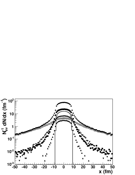
Figure 3: The same as in Fig. 2 for the Hubble-like parametrization.

In figures 2 and 3, we show the distributions of the $\pi^{+}$ emission transverse x-coordinate and time generated in the Bjorken-like and Hubble-like models with the parameters given in Table 1, $\eta_{\max}=2$. Also shown are the contributions from the primary $\pi^{+}$’s emitted directly from the freeze-out hypersurface and the contributions from $\pi^{+}$’s from the decays of the most abundant resonances $\rho$, $\omega$, $K^{*}(892)$ and $\Delta$. For primary pions, $x<R$ and $\tau<t<\tau\cosh\eta_{\max}$. The tails at $|x|>R$ and $t>\tau\cosh\eta_{\max}$ reflect the exponential law of the resonance decays. The longest tails in figures 2 and 3 are due to pions from $\omega$ decays.

VIII.3 Ratios of hadron abundances

It is well known that the particle abundances in heavy-ion collisions in a large energy range can be reasonably well described within statistical models (see, e.g., BHS95 ; Gorenstein97 ; THERMUS ) based on the assumption that the produced hadronic matter reaches thermal and chemical equilibrium. This is demonstrated in tables 2 and 3 for the particle number ratios near mid-rapidity in central Au +Au collisions at $\sqrt{s}_{NN}=130$ and 200 GeV calculated in our MC model and the statistical model of Ref. Bron02 and compared with the RHIC experimental data. Being independent of volume and flow parameters, the particle number ratio allow one to fix the thermodynamic parameters. We have not tuned the latter here and simply used the same thermodynamic parameters as in Ref. Bron02 despite there are noticeable differences in some particle number ratios calculated in the two models. These differences may be related to the different numbers of resonance states taken into account and uncertainties in the decay modes of high excited resonances.

Table 2: Particle number ratios near mid-rapidity in central Au + Au collisions at $\sqrt{s}_{NN}=130$ GeV calculated with the thermodynamic parameters: $T=0.168$ GeV, $\widetilde{\mu}_{B}=0.041$ GeV, $\widetilde{\mu}_{S}=0.010$ GeV and $\widetilde{\mu}_{Q}=-0.001$ GeV.

particle number ratios	our MC	statistical model Bron02	experiment
$\pi^{-}/\pi^{+}$	$0.98$	$1.02$	$1.00\pm 0.02$ 35 , $0.99\pm 0.02$ 36
$\bar{p}/\pi^{-}$	$0.06$	$0.09$	$0.08\pm 0.01$ 37
$K^{-}/K^{+}$	$0.90$	$0.92$	$0.91\pm 0.09$ 35 , $0.93\pm 0.07$ 39
$K^{-}/\pi^{-}$	$0.22$	$0.16$	$0.15\pm 0.02$ 40
$\bar{p}/p$	$0.61$	$0.65$	$0.60\pm 0.07$ 35 , $0.64\pm 0.08$ 39
$\bar{\Lambda}/\Lambda$	$0.69$	$0.69$	$0.71\pm 0.04$ 38
$\bar{\Xi}/\Xi$	$0.79$	$0.77$	$0.83\pm 0.06$ 38
$\phi/K^{-}$	$0.17$	$0.15$	$0.13\pm 0.03$ 41
$\Lambda/p$	$0.48$	$0.47$	$0.49\pm 0.03$ 42 , 43
$\Xi^{-}/\pi^{-}$	$0.0086$	$0.0072$	$0.0088\pm 0.0020$ 45

Table 3: Particle number ratios near mid-rapidity in central Au + Au collisions at $\sqrt{s}_{NN}=200$ GeV calculated with the thermodynamic parameters: $T=0.165$ GeV, $\widetilde{\mu}_{B}=0.028$ GeV, $\widetilde{\mu}_{S}=0.07$ GeV, and $\widetilde{\mu}_{Q}=-0.001$ GeV.

particle number ratios	our MC	experiment pt_PHENIX
$\pi^{-}/\pi^{+}$	$0.98$	$0.984\pm 0.004$
$K^{-}/K^{+}$	$0.94$	$0.933\pm 0.008$
$K^{-}/\pi^{-}$	$0.21$	$0.162\pm 0.001$
$\bar{p}/p$	$0.71$	$0.731\pm 0.011$

VIII.4 Pseudo-rapidity distributions

In Fig. 4, we compare the PHOBOS data eta_PHOBOS on pseudo-rapidity spectrum of charged hadrons in central Au+Au collisions at $\sqrt{s}_{NN}=200$ GeV with our MC results obtained within the Bjorken-like and Hubble-like models for different values of $\eta_{\max}$. One may see that the data are compatible with the longitudinal boost invariance only in the mid-rapidity region in which the model is practically insensitive to $\eta_{\max}$. In the single freeze-out scenario, the data on particle numbers at mid-rapidity thus allows one to fix the effective volume $V_{\rm eff}\propto\tau R^{2}$.

VIII.5 Transverse momentum spectra

In Fig. 5, we compare the mid-rapidity PHENIX data pt_PHENIX on $\pi^{+}$, $K^{+}$ and proton $p_{t}$ spectra in Au+Au collisions at $\sqrt{s}_{NN}=200$ GeV with our MC results obtained within the Bjorken-like and Hubble-like models. A good agreement between the models and the data may be seen for pions while for kaons and protons the models overestimate the spectra at $p_{t}<1$ GeV/$c$. For kaons, this discrepancy can be diminished with the help of the strangeness suppression parameter $\gamma_{s}$ of 0.8 (see the right panel in Fig. 5). The overestimated slope of the kaon and proton $p_{t}$ spectra can also be related with the oversimplified assumption of a common thermal and chemical freeze-out or insufficient number of the accounted heavy resonance states.

The contribution of different resonances to the pion $p_{t}$ spectrum calculated in the Bjorken-like model is shown in Fig. 6.

Note that in Hubble-like model, the transverse flow is determined by the volume parameters $R,\tau$ and so, at fixed thermodynamic parameters and the effective volume $V_{\rm eff}\propto\tau R^{2}$, the transverse momentum spectra allow one to fix both $R$ and $\tau$. In the Bjorken-like model, there is more freedom since the transverse flow is also regulated by the parameter $\rho_{u}^{\max}$. The choice of these parameters in Table 1 has been done to minimize the discrepancy of the simulated and measured correlation radii of identical pions (see below).

VIII.6 Correlation functions

It is well known that, due to the effects of quantum statistics (QS) and final state interaction (FSI), the momentum correlations of two or more particles at small relative momenta in their center-of-mass system are sensitive to the space-time characteristics of the production process on a level of fm $=10^{-15}$ m so serving as a correlation femtoscopy tool (see, for example, Lednicky05 -CF_STAR ).

The momentum correlations are usually studied with the help of correlation functions of two or more particles. Particularly, the two-particle correlation function $CF(p_{1},p_{2})$ is defined as a ratio of the measured two-particle distribution to the reference one which is usually constructed by mixing the particles from different events of a given class, normalizing the correlation function to unity at sufficiently large relative momenta.

Since our MC generator provides the information on particle four-momenta $p_{i}$ and four-coordinates $x_{i}$ of the emission points, it can be used to calculate the correlation function with the help of the weight procedure, assigning a weight to a given particle combination accounting for the effects of QS and FSI. Here we will consider the correlation function of two identical pions neglecting their FSI, so the weight

$$w=1+\cos(q\cdot\Delta x),$$ (47)

where $q=p_{1}-p_{2}$ and $\Delta x=x_{1}-x_{2}$. The $CF$ is defined as a ratio of the weighted histogram of the pair kinematic variables to the unweighted one.

Generally, the pair is characterized by six kinematic variables. In case of the azimuthal symmetry, there are five variables that are usually chosen as the three ”out-side-long” components of the relative three-momentum vector pod83 ; Pratt84 $\mathbf{q}=(q_{\mathrm{out}},q_{\mathrm{side}},q_{\mathrm{long}})$, half the pair transverse momentum $k_{t}$ and the pair rapidity or pseudo-rapidity. The out and side denote the transverse, with respect to the reaction axis, components of the vector ${\bf q}$; the out direction is parallel to the transverse component of the pair three–momentum.

The corresponding correlation widths are usually parameterized in terms of the Gaussian correlation radii $R_{i}$,

$$CF(p_{1},p_{2})=1+\lambda\exp(-R_{\mathrm{out}}^{2}q_{\mathrm{out}}^{2}-R_{\mathrm{side}}^{2}q_{\mathrm{side}}^{2}-R_{\mathrm{long}}^{2}q_{\mathrm{long}}^{2}-2R_{\mathrm{out,long}}^{2}q_{\mathrm{out}}q_{\mathrm{long}})$$ (48)

and their dependence on pair rapidity and transverse momentum is studied. The form of Eq. (48) assumes azimuthal symmetry of the production process pod83 . Generally, e.g., in case of the correlation analysis with respect to the reaction plane, all three cross terms $q_{i}q_{j}$ contribute Wiedemann_Heinz02 . We choose as the reference frame the longitudinal co-moving system (LCMS) cso91 . In LCMS each pair is emitted transverse to the reaction axis so that the pair rapidity vanishes. The parameter $\lambda$ measures the correlation strength. For fully chaotic Gaussian source $\lambda=1$. Experimentally observed values of $\lambda<1$ are mainly due to contribution of very long–lived sources ($\eta$, $\eta^{\prime}$, $K^{0}_{s}$, $\Lambda$, …), the non-Gaussian shape of the correlation functions and particle misidentification.

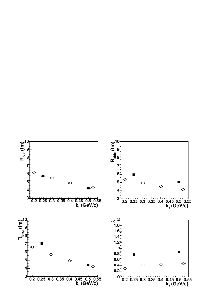
Figure 7: The $\pi^{\pm}\pi^{\pm}$ correlation radii and the suppression parameter $\lambda$ at mid-rapidity in central $Au+Au$ collisions at $\sqrt{s}_{NN}=200$ GeV from the STAR experiment CF_STAR (open circles) and the MC calculations within the Bjorken-like model (up-triangles) in different intervals of the pair transverse momentum $k_{t}$.

The correlation functions of two identical charged pions have been calculated within the Bjorken-like and Hubble-like models with the parameters given in Table 1, $\eta_{\max}=2$, reasonably well describing single particle spectra in the mid-rapidity region. The three-dimensional correlation functions were fitted according to Eq. (48) in two $k_{t}$ intervals $0.1<k_{t}<0.3$ GeV/$c$ and $0.3<k_{t}<0.6$ GeV/$c$. In Fig. 7, the fitted correlation radii and strength parameter are compared with those measured by STAR collaboration CF_STAR . One may see that the Bjorken-like model, adjusted to describe single particle spectra, describes also the decrease of the correlation radii with increasing $k_{t}$ but overestimates their values. The situation is even worth with the Hubble-like model which is more constraint than the Bjorken-like one and yields the longitudinal radius by a factor two larger.

As for the overestimation of the correlation strength parameter $\lambda$, it is likely related to the neglected contribution of misidentified particles and pions from weak decays. Indeed, the new preliminary analysis of the STAR data with the improved particle identification Bistr yields the $\lambda$ parameter closer to the model results.

We would like to emphasize that the high freeze-out temperature of $165$ MeV and a fixed effective volume $V_{\rm eff}\propto\tau R^{2}$ make it quite difficult to describe the correlation radii within the single freeze-out model. Thus a tuning of the longitudinal radius $R_{\rm long}\approx\tau(T/m_{t})^{1/2}$ requires a small proper time $\tau$, leading to too large values of $R$ and $R_{\rm side}\propto R$. The concept of a later thermal freeze-out occurring at a smaller temperature $T^{\rm th}<T^{\rm ch}$ and with no multiplicity constraint on the thermal effective volume (see section II) can help to resolve this problem (see, e.g., Lisa ).

To get a valuable information from the correlation data, one should consider more realistic models as compared with the simple Bjorken-like and Hubble-like ones (particularly, consider a more complex form of the freeze-out hypersurface taking into account particle emission from the surface of expanding system Borysova ) and study the problem of particle rescattering and resonance excitation after the chemical and/or thermal freeze-out (only minor effect of elastic rescatterings on particle spectra and correlations is expected UKM05 ). For the latter, our earlier developed C++ kinetic code UKM05 can be coupled to the MC freeze-out generator.

IX Conclusions and perspectives

We have developed a MC simulation procedure and the corresponding C++ code allowing for a fast but realistic description of multiple hadron production in central relativistic heavy ion collisions. A high generation speed and an easy control through input parameters make our MC generator code particularly useful for detector studies. As options, we have implemented two freeze-out scenarios with coinciding and with different chemical and thermal freeze-outs. Also implemented are various options of the freeze-out hypersurface parameterizations including those with non-space-like hypersurface sectors related to the emission from the surface of expanding system. The generator code is quite flexible and allows the user to add other scenarios and freeze-out surface parameterizations as well as additional hadron species in a simple manner.

We have compared the RHIC experimental data with our MC generation results obtained within the single freeze-out scenario and Bjorken-like and Hubble-like freeze-out surface parameterizations. While simplified, such a scenario nevertheless allows for a reasonable description of particle spectra. It however fails to describe the correlation functions of identical pions, overestimating the correlation radii.

The RHIC data thus points to the need for a more complicated scenario likely including different chemical and thermal freeze-outs, a more complex form of the freeze-out hypersurface (the use of numerical solution of the relativistic hydrodynamics is foreseen) and the account for kinetic evolution following the chemical and/or thermal freeze-out (for this, the MC generator can be coupled to our C++ kinetic code UKM05 ).

We plan to implement in the MC generator the impact parameter dependence of the freeze-out hypersurface and account for the anisotropic flow similar to Ref. Lokhtin03 ; Lokhtin05 . In view of the importance of high-$p_{t}$ physics related to the partonic states created in ultra-relativistic heavy ion collisions, we also foresee the inclusion of mini-jet production Lokhtin05 .

Figure 1: The validation of the MC procedure for $\rho_{u}^{\max}=0.65$ (left panel) and 2.0 (right panel): the transverse momentum spectra (solid lines) calculated according to Eq. (45) and the corresponding MC results (black triangles). Also shown are the MC results obtained with a constant residual weight (black points).

Figure 2: The $\pi^{+}$ emission transverse x-coordinate (left) and time (right) generated in the Bjorken-like model with the parameters given in Table 1, $\eta_{\max}=2$: all $\pi^{+}$’s (solid circles), direct $\pi^{+}$’s (solid line), decay $\pi^{+}$’s from $\rho$ (squares), $\omega$ (open circles), $K^{*}(892)$ (up-triangles) and $\Delta$ (down-triangles).

Figure 4: The pseudo-rapidity ($-\ln\tan(\theta/2)$, $\theta$ is the particle production angle) distributions of charged particles in central Au + Au collisions at $\sqrt{s}_{NN}=200$ GeV from the PHOBOS experiment eta_PHOBOS (solid circles) and the MC calculations within the Bjorken-like (left panel) and Hubble-like (right panel) models. The model results corresponding to the space-time rapidity range parameter $\eta_{\max}=5,3$ and 2 are shown by solid, dashed and dotted lines respectively.

Figure 5: The $\pi^{+}$, $K^{+}$ and proton transverse momentum spectra at mid-rapidity $y\approx 0$ in central Au + Au collisions at $\sqrt{s}_{NN}=200$ GeV from PHENIX experiment pt_PHENIX (solid symbols) and the MC calculations within the Bjorken-like (dashed lines) and Hubble-like (solid lines) models. The right panel shows the model results obtained with the strangeness suppression parameter $\gamma_{s}=0.8$.

Figure 6: The contributions to the $\pi^{+}$ transverse momentum spectrum at mid-rapidity in central Au + Au collisions at $\sqrt{s}_{NN}=200$ GeV calculated within the Bjorken-like model: all $\pi^{+}$’s (solid circles), direct $\pi^{+}$’s (stars), decay $\pi^{+}$’s from $\rho$ (squares), $\omega$ (open circles), $K^{*}(892)$ (up-triangles) and $\Delta$ (down-triangles).