${\bm{K}^{0}}$ photoproduction on the deuteron
and the extraction of the elementary amplitude

Abstract

The photoproduction of $K^{0}$ on the deuteron has been investigated with the inclusion of $YN$ and $KN$ final-state interaction (FSI), as well as the pion- mediated process $\gamma d\rightarrow\pi NN\rightarrow KYN$. The $YN$ rescattering effects for the inclusive cross section are found to be large in the threshold regions. Polarization observables show sizable FSI effects at larger kaon and hyperon angles. It is shown that the extraction of the elementary $\gamma N\rightarrow KY$ amplitude is possible in the quasi-free scattering region where FSI effects are negligible. Furthermore, the cross sections in this region are large, indicating that measurements in this kinematical region are favored.

I Introduction

In order to have a comprehensive understanding of the strong interaction, it is important to learn more about the hyperon-nucleon ($YN$) interaction. It could be studied through hyperon-nucleon scattering in a straightforward manner, though the lack of hyperon beams makes it difficult experimentally. Instead, kaon photoproduction on the deuteron offers itself as a suitable alternative for studying the hyperon-nucleon interaction in the final state. Several previous studies ReR67a ; ReR67b ; AdW89 ; LiW91 have been done in the inclusive and exclusive kaon photoproduction on the deuteron using simple $\Lambda n$ potentials. In a recent calculation Yamamura et al. YaM99 have investigated $YN$ final state interaction (FSI) effects of the $K^{+}$ channels using the more realistic Nijmegen $YN$ potentials MaR89 ; RiS99 . Sizeable FSI effects were found in both exclusive and inclusive cross sections, in particular near the $\Sigma$-threshold. They concluded that precise data would allow the study of the $YN$ interaction in a great detail. This work is extended in Ref. Sal03 with the inclusion of kaon-nucleon ($KN$) rescattering in the final state and the pion-mediated process $\gamma d\rightarrow\pi NN\rightarrow KYN$ ($\pi N-KY$ process for short) in the intermediate state. Other recent calculations Ker01 ; Max04 have also investigated these effects and reached similar conclusions.

Regarding kaon photoproduction on the nucleon, the most understood channels are the proton ones DaF96 ; Mar96 ; BeM96 ; MaB00 ; HaC01 ; JaR02 , i.e., $\gamma p\rightarrow K^{+}\Lambda$ and $\gamma p\rightarrow K^{+}\Sigma^{0}$, since a relatively large number of experimental data are available for these channels Boc94 ; Tra98 ; Goers:1999sw . Meanwhile, the study of neutron channels is needed in order to complete our understanding about kaon photoproduction on the nucleon. In these channels the elementary operator can be quite different. Because of isospin conservation at the hadronic vertices, there is no $\Lambda$ contribution in the intermediate states of the $\gamma n\rightarrow K^{+}\Sigma^{-}$ process. Furthermore, in the processes $\gamma n\rightarrow K^{0}\Lambda$ and $\gamma n\rightarrow K^{0}\Sigma^{0}$ there is no $t$-channel contribution in the Born terms since $K^{0}$ has zero electrical charge. Since free neutron targets are not available to study the neutron channels, one needs to use light nuclei like the deuteron or ³He as effective neutron targets. The deuteron is particularly well suited because of its small binding energy and its simple structure. Therefore, kaon photoproduction on the deuteron is the natural avenue in the investigation of kaon photoproduction on the neutron.

With the purpose of extracting the elementary cross section on the neutron target, Li et al. LiW92 have calculated the processes $d(\gamma,K^{0}p)\Lambda$, $d(\gamma,K^{0}p)\Sigma^{0}$, and $d(\gamma,K^{+}p)\Sigma^{-}$, where the kaon is detected in coincidence with the outgoing nucleon in the impulse approximation (IA). They concluded that, within the framework of their model, the deuteron can indeed be used to study $K^{0}$ and $K^{+}$ photoproduction from the neutron.

Very recently an experiment of $K^{0}$ photoproduction on the deuteron has been done at the Laboratory of Nuclear Science (LNS), in Sendai Hashimoto . They measured the cross section of the $d(\gamma,K^{0})\Lambda p$ process at a photon energy around 1.1 GeV with forward kaon angles. The data are now being analyzed. In the near future, they also plan to measure the cross section for the exclusive process and some polarization observables Maeda . Similarly, for the same reaction high-precision data from Jefferson Lab are being analyzed that have become available through the pentaquark searches pawel . In view of these experiments this paper extends the previous work YaM99 by calculating $K^{0}$ photoproduction on the deuteron and taking into account the effects of $KN$ rescattering and the $\pi N-KY$ process. Other rescattering processes (see, for example, Fig.2 in Max04 ) will not be included in our study, since for the kinematics considered here (close to quasi-free scattering or to the $YN$ thresholds) they do not contribute significantly. In extracting the elementary amplitude from the cross section we only consider the $\gamma d\rightarrow K^{0}\Lambda p$ channel, since the corresponding measurements have been performed. In Sect. II, we briefly review the production operator used in this work. The formalism for calculating the transition matrix and observables are shown in Sect. III. The results are presented in Sect. IV and we close the paper with conclusions in Sect. V.

II The kaon photoproduction operator

Most analyses of kaon photoproduction on the nucleon have been performed at tree level in an effective Lagrangian approach. While this leads to violation of unitarity, this kind of isobar model provides a simple tool to parameterize the elementary process because it is relatively easy to calculate and to use for production on nuclei. In this approach, the photoproduction amplitude $\gamma N\rightarrow KY$ ( in the following denoted as elementary amplitude) can be written as

$$\langle\vec{p}_{Y}\mu_{Y}|t^{\gamma K}_{\lambda}|\vec{p}_{N}\mu_{N}\rangle = \bar{u}_{\mu_{Y}}\Big{(}\sum_{i=1}^{4}A_{i}\Gamma^{i}_{\lambda}\Big{)}u_{\mu_{N}}\,,~{}~{}$$ (1)

where $A_{i}$’s are invariant amplitudes as functions of the Mandelstam variables only. The hyperon and nucleon Dirac spinors are denoted by $u_{\mu_{Y}}$ and $u_{\mu_{N}}$, respectively. The invariant Dirac operators $\Gamma^{i}_{\lambda}$, which are given by

$$\Gamma^{1}_{\lambda} = {\textstyle\frac{1}{2}}\gamma_{5}\left({\epsilon\!\!/}\!_{\lambda}k\!\!\!/-k\!\!\!/{\epsilon\!\!/}\!_{\lambda}\right)\,,$$ (2)

$$\Gamma^{2}_{\lambda} = \gamma_{5}\left[(2q-k)\cdot\epsilon_{\lambda}P\cdot k-(2q-k)\cdot kP\cdot\epsilon_{\lambda}\right]\,,$$ (3)

$$\Gamma^{3}_{\lambda} = \gamma_{5}\left(q\cdot k{\epsilon\!\!/}\!_{\lambda}-q\cdot\epsilon_{\lambda}k\!\!\!/\right)\,,$$ (4)

$$\Gamma^{4}_{\lambda} = i\epsilon_{\mu\nu\rho\sigma}\gamma^{\mu}q^{\nu}\epsilon^{\rho}_{\lambda}k^{\sigma}\,,$$ (5)

are gauge invariant Lorentz pseudoscalars and given in terms of the usual $\gamma$-matrices, the photon momentum $k$, and its polarization vector $\epsilon_{\lambda}$. Here $\lambda$ labels the polarization states, $q$ the meson momentum, and $P=(p^{\prime}+p)/2$, where $p$ and $p^{\prime}$ denote initial and final baryon momenta, respectively Don72 . By expressing the Dirac operators and spinors in term of Pauli matrices $\vec{\sigma}$ and spinors $\chi$, we can write the kaon photoproduction operator as

$$t^{\gamma K}_{\lambda} = i\Big{(}L_{\lambda}+i\vec{\sigma}\cdot\vec{K}_{\lambda}\Big{)}\,,$$ (6)

where $L_{\lambda}$ and $\vec{K}_{\lambda}$ are functions of $A_{i}$. The rather lengthy expression of $A_{i}$, $L_{\lambda}$, and $\vec{K}_{\lambda}$ can be found in Ref. Mar96 .

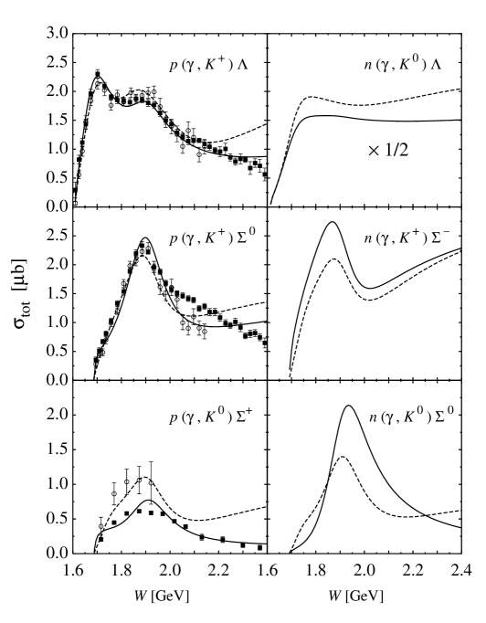
Figure 1: Total cross section of kaon photoproduction on the nucleon obtained by using the original KAON-MAID model (dashed lines) and the same model but refitted to the new SAPHIR data (solid lines). Older experimental data are taken from Refs. Tra98 ; Goers:1999sw , while new SAPHIR data are taken from Refs. Lawall:2005np ; Glan03b .

In the present work we use the KAON-MAID model MaB00 , which includes the $D_{13}$(1895) resonance beside the Born terms and other resonances. Separate hadronic form factors for each vertex were used. In order to restore gauge invariance, the recipe from Haberzettl Hab97 was utilized. The coupling constants and cut-off parameters were determined by fitting to the experimental data. The behavior of this model in all six isospin channels is exhibited by the dashed lines in Fig. 1.

Recently, the SAPHIR collaboration at ELSA has published new data on all proton channels, i.e. the $\gamma p\rightarrow K^{+}\Lambda$, $\gamma p\rightarrow K^{+}\Sigma^{0}$ and $\gamma p\rightarrow K^{0}\Sigma^{+}$ ones. The new data are more precise and cover all angular distributions in the energy range from threshold up to $W\simeq 2.4$ GeV. Furthermore, as shown by the middle- and lower-left panels of Fig. 1, these new data show a significant discrepancy with the previous experiment in the $\gamma p\rightarrow K^{+}\Sigma^{0}$ and $\gamma p\rightarrow K^{0}\Sigma^{+}$ channels. Since KAON-MAID was fitted to previous data, it obviously faces a problem to reproduce the new ones. Figure 1 reveals this problem explicitly.

To investigate the effects of new data on KAON-MAID we refit the coupling constants in this isobar model by only using the new SAPHIR data in our database. The results are shown by the solid lines in Fig. 1. While in the $\gamma p\rightarrow K^{+}\Lambda$ and $\gamma p\rightarrow K^{0}\Sigma^{+}$ channels KAON-MAID can nicely reproduce the new measurements, it is obviously unable to explain the $\gamma p\rightarrow K^{+}\Sigma^{0}$ cross section at $W\gtrsim 2.0$ GeV. This problem originates from the fact that KAON-MAID does not have certain resonances at this energy region. By floating the resonance masses during the fit process, a recent study has shown that the new data on this channel demand a nucleon resonance $S_{11}$ with $M\simeq 2100$ MeV Lawall:2005np .

The predicted total cross sections for neutron channels are given in the three right panels of Fig. 1. There are sizable differences between the original prediction of KAON-MAID and the refitted version. Nevertheless, all predicted cross sections are of the same order.

Very recently, the CLAS collaboration has also published their data for both $\gamma p\rightarrow K^{+}\Lambda$ and $\gamma p\rightarrow K^{+}\Sigma^{0}$ channels McNabb:2003nf ; Bradford:2005pt . The CLAS data show, unfortunately, substantial and systematic discrepancies with the SAPHIR ones. This problem is clearly illustrated in Fig. 2. As a consequence, an effort to simultaneously fit the model to both data versions would be meaningless. In view of this, we decide to use the original KAON-MAID model in the subsequent calculations. This choice is also supported by the fact that in this paper most calculations on the deuteron have been performed at low photon energy, a region where the original and the refitted KAON-MAID models are still in good agreement and the discrepancy in the new experimental data is not too significant. Furthermore, our main motivation in this paper is to show the possibility to extract the elementary cross section for the $\gamma N\rightarrow KY$ process from the deuteron cross section. Therefore, we can expect that the main conclusion will be independent from the choice of elementary model.

Figure 2: Example of the systematic discrepancy between SAPHIR (open squares) Lawall:2005np and CLAS (solid squares) McNabb:2003nf data in the differential cross section of the $\gamma p\rightarrow K^{+}\Lambda$ channel as a function of the total c.m. energy $W$. Predictions from the two elementary operator models given in Fig. 1 are shown for comparison.

III The reaction on the deuteron

III.1 Cross sections and amplitudes

The general expression for the cross section using the convention of Bjorken and Drell BjDr is given by

$$d\sigma = \frac{1}{|\vec{v}_{\gamma}-\vec{v}_{d}|}\frac{m_{Y}m_{N}}{8E_{\gamma}E_{K}E_{d}E_{Y}E_{N}}\frac{d\vec{p}_{K}}{(2\pi)^{3}}\frac{d\vec{p}_{Y}}{(2\pi)^{3}}\frac{d\vec{p}_{N}}{(2\pi)^{3}}\,(2\pi)^{4}\delta^{4}(P_{d}+Q-p_{Y}-p_{N})\,$$ (7)

$$\times\,\frac{1}{6}\sum_{\mu_{Y}\mu_{N}\mu_{d}\lambda}\big{|}\sqrt{2}\langle\vec{p}_{Y}\vec{p}_{N}\mu_{Y}\mu_{N}|T^{\gamma K}_{\lambda}|\Psi_{\mu_{d}}\rangle\,\big{|}^{2}\,,$$

where $\mu_{Y}$, $\mu_{N}$, $\mu_{d}$, and $\lambda$ denote the spin projections of hyperon, nucleon, deuteron and the photon polarization, respectively. For the deuteron state $\Psi_{\mu_{d}}$, however, we use a noncovariant notation, which removes the standard additional factor $1/2E_{d}(2\pi)^{3}$. Here $Q=p_{\gamma}-p_{K}$ is the momentum transfer to the two-baryon system and the factor $\sqrt{2}$ comes from the proper antisymmetrization. In this expression the dependencies on the kinematical variables have been suppressed and it should be understood that the production operator acts on one of the two initial baryons. By integrating the right hand side of Eq. (7) over the three-momentum of nucleon and momentum of hyperon, followed by rewriting the flux factor, we arrive at the cross section for the exclusive process $d(\gamma,KY)N$ in the deuteron rest frame, i.e.,

$$\frac{d\sigma}{dp_{K}d\Omega_{K}d\Omega_{Y}} = \frac{m_{Y}m_{N}|\vec{p}_{K}|^{2}|\vec{p}_{Y}|^{2}}{4(2\pi)^{2}E_{\gamma}E_{K}}\,\big{|}(E_{Y}+E_{N})|\vec{p}_{Y}|-E_{Y}\vec{Q}\cdot\hat{p}_{Y}\big{|}^{-1}\,$$ (8)

$$\times\,\frac{1}{6}\sum_{\mu_{Y}\mu_{N}\mu_{d}\lambda}\big{|}\sqrt{2}\langle\vec{p}_{Y}\vec{p}_{N}\mu_{Y}\mu_{N}|T^{\gamma K}_{\lambda}|\Psi_{\mu_{d}}\rangle\big{|}^{2}\,.$$

Through out the paper we work in the deuteron rest frame. For the inclusive process $d(\gamma,K)YN$ the cross section is given by

$$\frac{d\sigma}{dp_{K}d\Omega_{K}} = \int d\Omega^{\,\rm cm}_{Y}\,\frac{m_{Y}m_{N}|\vec{p}_{K}|^{2}|\vec{p}^{\,\rm cm}_{Y}|}{4(2\pi)^{2}E_{\gamma}E_{K}W}\,$$ (9)

$$\times\,\frac{1}{6}\sum_{\mu_{Y}\mu_{N}\mu_{d}\lambda}\big{|}\sqrt{2}\langle\vec{p}_{Y}\vec{p}_{N}\mu_{Y}\mu_{N}|T^{\gamma K}_{\lambda}|\Psi_{\mu_{d}}\rangle\,\big{|}^{2}\,,$$

where $W^{2}=(P_{d}+Q)^{2}$ and $|\vec{p}^{\,\rm cm}_{Y}|$ is the hyperon momentum calculated in the center of mass frame of the two final baryons.

The amplitude is approximated by the diagram shown in Fig. 3, which is written for convenience as

$$T^{\gamma K}_{\lambda} = t^{\gamma K}+t^{\gamma K}_{YN}+t^{\gamma K}_{KN}+t^{\gamma K}_{K\pi}\,,$$ (10)

where $t^{\gamma K}$, $t^{\gamma K}_{YN}$, $t^{\gamma K}_{KN}$, and $t^{\gamma K}_{K\pi}$ denote the operators for the impulse approximation, hyperon-nucleon rescattering, kaon-nucleon rescattering, and the pion mediated process, respectively.

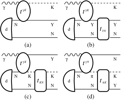
Figure 3: Kaon photoproduction on the deuteron. The diagrams indicate (a) the impulse approximation (IA), (b) the $YN$ rescattering, (c) the $KN$ rescattering, and (d) the $\pi N-KY$ process.

The IA and $YN$ rescattering terms are calculated precisely. Here we describe the calculation briefly; the reader should consult Ref. YaM99 for details. The operator of the sum of diagrams (a) and (b) can be written as

$$T^{\gamma K}_{YN} = t^{\gamma K}+t^{\gamma K}_{YN}$$ (11)

$$= t^{\gamma K}+t_{YN}\,G_{YN}t^{\gamma K}\,$$ (12)

with the $YN$ scattering operator $t_{YN}$ which obeys the Lippmann-Schwinger equation

$$t_{YN} = V_{YN}+V_{YN}\,G_{YN}\,t_{YN}\,,$$ (13)

where $V_{YN}$ denotes the $YN$ potential operator and $G_{YN}$ the free $YN$ propagator. Inserting Eq. (13) into Eq. (12), we obtain

$$T^{\gamma K}_{YN} = t^{\gamma K}+V_{YN}\,G_{YN}\,T^{\gamma K}_{YN}\,,$$ (14)

which can be solved by inversion, i.e.,

$$T^{\gamma K}_{YN} = \left(1-V_{YN}\,G_{YN}\right)^{-1}t^{\gamma K}\,.$$ (15)

After solving the last equation in a partial wave decomposition with respect to the $YN$ subsystem, one obtains the $YN$ rescattering amplitude by subtraction of the IA term.

The $KN$ rescattering (diagram (c) in Fig. 3) is evaluated directly in contrast to $YN$ rescattering. The corresponding operator is given by

$$t^{\gamma K}_{KN} = t_{KN}\,G_{KN}\,t^{\gamma K}\,,$$ (16)

where $t_{KN}$ is the $KN$ scattering operator, which also obeys the Lippmann-Schwinger equation of the form (13), and $G_{KN}$ is the free $KN$ propagator. For $V_{KN}$ we take a rank-1 separable potential which, in the partial wave representation, is given by

$$V_{\ell J}(p^{\prime},p) = \lambda_{\ell J}\,g(p^{\prime})_{\ell J}\,g(p)_{\ell J}$$ (17)

with the form factor

$$g(p)_{\ell J} = \frac{B_{\ell J}\,p^{\ell}}{\left[p^{2}+A_{\ell J}^{2}\right]^{\frac{\ell+2}{2}}}\,,$$ (18)

where $\lambda_{\ell J}$, $B_{\ell J}$, and $A_{\ell J}$ are parameters which are determined by fitting the phase shift to the experimental data HyA92 ; Sax80 . The $\pi N-KY$ process (diagram (d) in Fig. 3) is calculated in the same fashion; details of these calculations can be found in Ref. Sal03 .

III.2 Polarization Observables

With respect to polarization observables, we consider the tensor target asymmetries $T_{2M}$ which are given by Are88

$$T_{2M}\frac{d\sigma}{d\Omega_{K}} = (2-\delta_{M0})\,{\mathcal{R}e}\,V_{2M}\,,\quad M=0,1,2\,,$$ (19)

where

$$V_{2M} = \sqrt{15}\sum_{\mu_{Y}\mu_{N}\lambda}\sum_{\mu^{\prime}_{d}\mu_{d}}(-1)^{1-\mu^{\prime}_{d}}\left(\begin{array}[]{ccc}1&1&2\\ \mu_{d}&-\mu^{\prime}_{d}&-M\end{array}\right)$$ (23)

$$\times\,\int_{p_{K}^{\rm min}}^{p_{K}^{\rm max}}dp_{K}\int d\Omega^{\,\rm cm}_{Y}\,\kappa\,{\cal M}_{\mu_{Y}\mu_{N}\mu_{d}\lambda}^{*}{\cal M}_{\mu_{Y}\mu_{N}\mu^{\prime}_{d}\lambda}$$

with a kinematic factor

$$\kappa = \frac{m_{Y}m_{N}|\vec{p}_{K}|^{2}|\vec{p}^{\,\rm cm}_{Y}|}{24(2\pi)^{2}E_{\gamma}E_{K}W}\,.$$ (24)

We also calculate the hyperon recoil polarization $P_{y}$, the beam asymmetry $\Sigma$, and the double polarization $C_{x}$ and $C_{z}$, which are given by

$$P_{y} = \frac{{\rm Tr}\,{\cal M}{\cal M}^{+}\sigma_{y}}{{\rm Tr}\,{\cal M}{\cal M}^{+}}\,,$$ (25)

$$\Sigma = \frac{{\rm Tr}\,{\cal M}_{\epsilon_{y}}{\cal M}^{+}_{\epsilon_{y}}-{\rm Tr}\,{\cal M}_{\epsilon_{x}}{\cal M}^{+}_{\epsilon_{x}}}{{\rm Tr}\,{\cal M}_{\epsilon_{y}}{\cal M}^{+}_{\epsilon_{y}}+{\rm Tr}\,{\cal M}_{\epsilon_{x}}{\cal M}^{+}_{\epsilon_{x}}}\,,$$ (26)

$$C_{x} = \frac{{\rm Tr}\,{\cal M}_{\epsilon_{1}}{\cal M}^{+}_{\epsilon_{1}}\sigma_{x}}{{\rm Tr}\,{\cal M}_{\epsilon_{1}}{\cal M}_{\epsilon_{1}}}\,,$$ (27)

$$C_{z} = \frac{{\rm Tr}\,{\cal M}_{\epsilon_{1}}{\cal M}^{+}_{\epsilon_{1}}\sigma_{z}}{{\rm Tr}\,{\cal M}_{\epsilon_{1}}{\cal M}_{\epsilon_{1}}}\,.$$ (28)

In these equations the amplitude ${\cal M}$ reads

$$\cal M = \sqrt{2}\,\langle\vec{p}_{Y}\vec{p}_{N}\mu_{Y}\mu_{N}|T^{\gamma K}_{\lambda}|\Psi_{\mu_{d}}\rangle\,,$$ (29)

where, for example, ${\cal M}_{\epsilon_{y}}$ indicates the amplitude with photon polarization pointing into the y-axis, i.e. $\vec{\epsilon}_{\lambda}$ = $\vec{\epsilon}_{y}$. The photon polarization $\vec{\epsilon}_{1}$ = $-\frac{1}{\sqrt{2}}(\vec{\epsilon}_{x}+i\vec{\epsilon}_{y})$ describes the helicity state +1. The beam asymmetry $\Sigma$ is obtained with linearly polarized photon, while the double polarization observables $C_{x}$ and $C_{z}$ are the observables for both polarized hyperon and circularly polarized photon.

III.3 Extraction of the elementary amplitude

In the following, we describe briefly the extraction of the invariant elementary amplitude from the cross section on the deuteron in view of the study of kaon photoproduction on the neutron. The condition for the extraction must be that FSI effects be negligible. Thus, the amplitude can be approximated only by the impulse term. In this case the invariant elementary amplitude can be separated from the deuteron one. To show this, first we write the amplitude of the impulse term explicitly as

$$\mbox{$\langle\vec{p}_{Y}\vec{p}_{N}\mu_{Y}\mu_{N}|$}t^{\gamma K}_{\lambda}\mbox{$|\Psi_{\mu_{d}}\rangle$} = \sum_{\mu_{N^{\prime}}}\mbox{$\langle\vec{p}_{Y}\mu_{Y}|$}t^{\gamma K}_{\lambda}\mbox{$|-\vec{p}_{N}\mu_{N^{\prime}}\rangle$}\,C^{\frac{1}{2}\,\frac{1}{2}\,1}_{\mu_{N}\mu_{N^{\prime}}\mu_{S}}\Psi_{\mu_{S}\mu_{d}}(-\vec{p}_{N})\,,$$ (30)

where $C$ denotes Clebsch-Gordan coefficient and $\vec{p}_{N}$ is the spectator nucleon momentum. The deuteron wave function $\Psi$ is given by

$$\Psi_{\mu_{S}\mu_{d}}(-\vec{p}_{N}) = \sum_{\ell}C^{\ell\,1\,1}_{\mu_{\ell}\mu_{S}\mu_{d}}\,u_{\ell}(|\vec{p}_{N}|)\,Y_{\ell\mu_{\ell}}(-\hat{p}_{N})\,,$$ (31)

where $Y$ indicates spherical harmonics and $u$ is its radial part, which is generated by the Nijmegen93 NN potential nij93 in this work. Summing over all spin states of the amplitude in Eq. (30), after some algebra we find

$$\sum_{\mu_{Y}\mu_{N}\mu_{d}\lambda}\big{|}\mbox{$\langle\vec{p}_{Y}\vec{p}_{N}\mu_{Y}\mu_{N}|$}t^{\gamma K}_{\lambda}\mbox{$|\Psi_{\mu_{d}}\rangle$}\big{|}^{2} = D\,\sum_{\mu_{Y}\mu_{N^{\prime}}\lambda}\big{|}\mbox{$\langle\vec{p}_{Y}\mu_{Y}|$}t^{\gamma K}_{\lambda}\mbox{$|-\vec{p}_{N}\mu_{N^{\prime}}\rangle$}\big{|}^{2}\,,$$ (32)

where

$$D = {\textstyle\frac{3}{2}}|Y_{00}|^{2}u_{0}^{2}+\left({\textstyle\frac{3}{10}}|Y_{20}|^{2}+{\textstyle\frac{3}{5}}|Y_{21}|^{2}+{\textstyle\frac{3}{5}}|Y_{22}|^{2}\right)u_{2}^{2}\,.$$ (33)

With this expression we can write Eq. (8) as

$$\frac{d\sigma}{dp_{K}d\Omega_{K}d\Omega_{Y}} = \frac{m_{Y}m_{N}|\vec{p}_{K}|^{2}|\vec{p}_{Y}|^{2}}{4(2\pi)^{2}E_{\gamma}E_{K}}\,\big{|}(E_{Y}+E_{N})|\vec{p}_{Y}|-E_{Y}\vec{Q}\cdot\hat{p}_{Y}\big{|}^{-1}\,$$ (34)

$$\times\,\frac{1}{6}\,D\sum_{\mu_{Y}\mu_{N^{\prime}}\lambda}\big{|}\mbox{$\langle\vec{p}_{Y}\mu_{Y}|$}t^{\gamma K}_{\lambda}\mbox{$|-\vec{p}_{N}\mu_{N^{\prime}}\rangle$}\big{|}^{2}\,.$$

On the r.h.s. of this equation the sum of the squared amplitudes of the elementary process $\gamma N\rightarrow KY$ has been completely separated from the deuteron wave function.

IV Results

Figure 4: Inclusive cross sections of $d(\gamma,K^{0})YN$ as functions of $p_{K}$ at $E_{\gamma}=1.1$ GeV and $\theta_{K}=0^{\circ}$. The dashed line denotes the IA results and the solid line the IA+$YN$ results. The arrow indicates the $\Sigma$ threshold.

Figure 5: Comparison of the inclusive cross sections in IA using the two different elementary models given in Fig 1.

The inclusive cross section, calculated using Eq. (9) at a photon energy of $E_{\gamma}$ = 1.1 GeV and at forward kaon angle $\theta_{K}=0^{\circ}$, is shown in Fig. 5. In this figure we add up the cross section for all outgoing channels, $K^{0}\Lambda p$, $K^{0}\Sigma^{0}p$ and $K^{0}\Sigma^{+}n$. The positions of the two peaks are found to be consistent with the $\Lambda$ and $\Sigma$ quasi-free scattering (QFS) conditions. We note sizable effects of $YN$-rescattering in the $\Lambda$ and $\Sigma$ threshold regions, and on the top of the $\Lambda$-peak around $p_{K}=690$ MeV/$c$. Figure 5 shows the inclusive cross sections in IA, where the results for the two different elementary operators discussed in Sec. II are compared. This figure shows a relatively large variation of the cross sections around the $\Sigma$-QFS region. This result originates from the different models for the elementary process (see Fig. 1) of the $K^{+}\Sigma^{-}$ channel at this energy of $W\simeq 1.7$ GeV. The other $K\Sigma$ channels also exhibit significant differences, but since their overall cross sections are smaller compared to $K^{+}\Sigma^{-}$, their effects become less important. In contrast to the $K^{+}\Sigma^{-}$ channel, for both the $K^{+}\Lambda$ and $K^{0}\Lambda$ channels the corresponding cross sections do not differ too much around $W=1.7$ GeV. This also explains why the difference between the two elementary models does not show up strongly around the $\Lambda$-QFS region.

By comparing Figs.  5 and 5, we can see that the variation originating from the different elementary operators is larger than that originating from the FSI effects around the $\Sigma$-QFS region. In other words, we can say that the cross section of the process $d(\gamma,K^{0})\Sigma N$ is more sensitive to the choice of the elementary operators than to the FSI effects. This feature shows that the process $d(\gamma,K^{0})\Sigma N$ can serve as a way to access the elementary operators. Experimental data with error bars smaller than these variations are needed now to apply our procedure.

Figure 6: Exclusive cross sections as a function of hyperon angle $\theta_{Y}$ for $\gamma d\rightarrow K^{0}\Lambda p$ (left panels), and $\gamma d\rightarrow K^{0}\Sigma^{0}p$ (right panels) at the photon energy $E_{\gamma}$ = 1.1 GeV, kaon angle $\theta_{K}=0^{\circ}$, hyperon angle $\phi_{Y}=0^{\circ}$ for two values of the kaon momentum $\vec{p}_{K}$. The dotted line corresponds to IA, the short-dashed line to IA+$YN$, the dashed line to IA+$YN$+$KN$, and the solid line to IA+$YN$+$KN$+($\pi N-KY$).

Figure 7: Tensor asymmetries $T_{20}$, $T_{21}$, and $T_{22}$, as a function of kaon angle $\theta_{K}$ for $\gamma d\rightarrow K^{0}\Lambda p$ (left panels), and $\gamma d\rightarrow K^{0}\Sigma^{0}p$ (right panels) for the photon energy $E_{\gamma}$ = 1.1 GeV. The lines are as in Fig. 7.

Figure 7 presents the exclusive cross sections calculated for the photon energy 1.1 GeV at forward kaon angle $\theta_{K}=0^{\circ}$. The figure shows that the effect of the $YN$ rescattering is stronger at larger hyperon angles, while the effects of $KN$ rescattering and $\pi N-KY$ process are negligible or small.

The tensor asymmetries for the photon energy of $E_{\gamma}$ = 1.1 GeV are shown in Fig. 7. This figure shows that the $YN$, $KN$ rescatterings, and $\pi N-KY$ process have different effects on $T_{20}$, $T_{21}$, and $T_{22}$ at larger kaon angles.

Figure 8: Beam asymmetry $\Sigma$, recoil polarization $P_{y}$, and double polarizations $C_{x}$ and $C_{z}$, as functions of the hyperon angle $\theta_{Y}$ for the $\gamma d\rightarrow K^{0}\Lambda p$ process. Top and bottom panels are for the two kaon momenta $p_{K}=690$ and 590 MeV/$c$, respectively. The photon energy is $E_{\gamma}$ = 1.1 GeV, the kaon angle is fixed at $\theta_{K}=0^{\circ}$ and the hyperon azimuthal angle is $\phi_{Y}=0^{\circ}$. The lines are as in Fig. 7.

Figure 9: Same as in Fig. 8 but for $\gamma d\rightarrow K^{0}\Sigma^{0}p$ with $p_{K}=520$ and 420 MeV/$c$.

Figures 8 and 9 show the polarization observables $\Sigma$, $P_{y}$, $C_{x}$, and $C_{z}$ in the $\gamma d\rightarrow K^{0}\Lambda p$ and $\gamma d\rightarrow K^{0}\Sigma^{0}p$ channels, respectively. These polarization observables are calculated for the photon energy $E_{\gamma}$ = 1.1 GeV, the kaon angle $\theta_{K}=0^{\circ}$, and the hyperon angle $\phi_{Y}=0^{\circ}$. The top panels correspond to the results at the peak positions of the inclusive cross section, while the bottom panels refer to lower kaon momenta. For these observables the $YN$ rescattering effects dominate at larger hyperon angles $\theta_{Y}$. The effects are more remarkable at lower kaon momenta than at the peak positions.

Figure 10: Exclusive cross sections of $d(\gamma,K^{0}\Lambda)p$ as functions of kaon angle $\theta_{K}$ for the photon energy $E_{\gamma}$ = 1.1 GeV. The direction of the outgoing nucleon momentum $\vec{p}_{N}$ is fixed at $\theta_{N}=30^{\circ}$ and $\phi_{N}=180^{\circ}$, but the magnitude of $\vec{p}_{N}$ is varied. The results for $p_{N}=0$, 50, 100, and 150 MeV/$c$ are shown. The lines are as in Fig. 7.

Figure 11: Same as Fig. 11 but for the photon energy $E_{\gamma}$ = 1.3 GeV.

Figure 12: Comparison between the extracted and the free-process amplitudes squared for the process $\gamma n\rightarrow K^{0}\Lambda$ at the photon energy $E_{\gamma}$ = 1.1 GeV (left panels) and $E_{\gamma}$ = 1.3 GeV (right panels). The solid line refers to the extracted amplitudes from $\gamma d\rightarrow K^{0}\Lambda p$, while the dashed line is obtained from the free-process amplitudes. The direction of $\vec{p}_{N}$ is fixed at $\theta_{N}=30^{\circ}$ and $\phi_{N}=180^{\circ}$, but the magnitude of $\vec{p}_{N}$ is varied with 0, 50, 100 150 MeV/$c$.

Figures 11 and 11 show the exclusive cross sections of $d(\gamma,K^{0}\Lambda)p$ as a function of kaon angle $\theta_{K}$ for the photon energies $E_{\gamma}$ = 1.1 and 1.3 GeV, respectively. In the figures we fix the direction of the outgoing nucleon momentum $\vec{p}_{N}$ to $\theta_{N}=30^{\circ}$ and $\phi_{N}=180^{\circ}$, while several magnitudes of $\vec{p}_{N}$, namely 0, 50, 100, and 150 MeV/$c$ are studied. At nucleon momentum $p_{N}=150$ MeV/$c$, the effects of $YN$ rescattering are most prominent at forward kaon angles, but almost negligible for zero nucleon momentum, i.e. under QFS kinematics. From these features we conclude that the extraction of the elementary amplitude is favored in QFS kinematics.

Finally, in Fig. 12 we compare the extracted elementary amplitudes for $p_{N}=0$, 50, 100 MeV/$c$ with the corresponding free-process amplitudes. We see that the extracted amplitudes are in good agreement with the free-process amplitudes at QFS kinematics. At $p_{N}=50$ MeV/$c$ there is a small discrepancy between the extracted and the free-process amplitudes, especially at larger kaon angles. The discrepancy grows at $p_{N}=100$ MeV/$c$. One can also note from the figures that the extraction works better done at higher photon energies $E_{\gamma}$ where the discrepancy is smaller for the same nucleon momentum $p_{N}$.

Figure 13: Three dimensional plot of $d(\gamma,K^{0})YN$ as a function of $\theta_{K}$ and $p_{K}$, which is obtained with IA + YN. The photon energy is $E_{\gamma}$ = 1.1 GeV.

Another feature visible in Figs. 11 and 11 is that the cross section of the exclusive process $d(\gamma,K^{0}\Lambda)p$ in QFS kinematics is much larger than in other kinematic regions, indicating that measurements in this region will be easier. For visualizing the QFS regions over a wide range of $p_{K}$ and $\theta_{K}$, we provide a three-dimensional plot of the inclusive process $d(\gamma,K^{0})\Lambda p$ obtained with IA + YN in Fig. 13, for the photon energy $E_{\gamma}$ = 1.1 GeV. This figure shows a ridge running along the QFS condition which moves to smaller kaon momentum $p_{K}$ as the kaon angle $\theta_{K}$ increases.

V Summary and Conclusion

We have analyzed $K^{0}$ photoproduction on the deuteron $\gamma d\rightarrow KYN$, investigating the effects of $YN$ and $KN$ rescattering and the intermediate $\pi N-KY$ rescattering process. $YN$ rescattering effects are found to be large in the threshold regions in the inclusive cross section for forward kaon angle $\theta_{K}=0^{\circ}$. The two models of KAON-MAID for the elementary operator, the original and the refitted one to the new SAPHIR data, show a large variation in the $\Sigma$ QFS region of the inclusive cross sections. Therefore, the $d(\gamma,K^{0})YN$ experiments can serve as a method to access those operators. In the exclusive processes, the polarization observables show visible effects of the final-state interactions at larger hyperon angles.

We have also calculated the exclusive cross section for outgoing nucleon momenta $\vec{p}_{N}$ with various magnitudes in a fixed direction. The $YN$ rescattering effects are found to become larger at forward kaon angles as the magnitude of $\vec{p}_{N}$ increases, but those are almost negligible at zero nucleon momentum, i.e. under QFS kinematics. We have shown that the elementary amplitude can be extracted algebraically from the full amplitude using the impulse approximation when FSI effects do not contribute. We have performed the extraction for the $\vec{p}_{N}$-values mentioned above, and the extracted elementary amplitudes have been compared with the free-process ones. At QFS kinematics the extracted and the free-process amplitudes agree well. This demonstrates that kaon photoproduction on the deuteron in the QFS region is suitable for investigating the elementary process in the neutron channels. The exclusive cross sections for the $d(\gamma,K^{0}\Lambda)p$ process at the QFS kinematics are found to be especially large suggesting that this region is appropriate for measurements. We confirm that the region where the cross sections are large develops close to QFS kinematics and forms a ridge on the $\theta_{K}-p_{K}$ plane.

References

• (1) F.M. Renard and Y. Renard, Nucl. Phys. B1, 389 (1967).
• (2) F.M. Renard and Y. Renard, Phys. Lett. B24, 159 (1967).
• (3) R.A. Adelseck and L.E. Wright, Phys. Rev. C 39, 580 (1989).
• (4) X. Li and L.E. Wright, J. Phys. G 17, 1127 (1991).
• (5) H. Yamamura, K. Miyagawa, T. Mart, C. Bennhold, W. GlΓΆckle, and H. Haberzettl, Phys. Rev. C 61, 014001 (1999).
• (6) P.M.M. Maessen, Th.A. Rijken, and J.J. de Swart, Phys. Rev. C 40, 2226 (1989).
• (7) Th.A. Rijken, V.G.J. Stoks, and Y. Yamamoto, Phys. Rev. C 59, 21 (1999).
• (8) A.Salam and H.ArenhΓΆvel, Phys. Rev. C 70, 044008 (2004); A. Salam, Dissertation, Johannes Gutenberg UniversitΓ€t, Mainz, 2003 ( unpublished).
• (9) B.O. Kerbikov, Phys. Atom. Nucl. 64, 1835 (2001).
• (10) O.V. Maxwell, Phys. Rev. C 69, 034605 (2004).
• (11) J.C. David, C. Fayard, G.H. Lamot, and B. Saghai, Phys. Rev. C 53, 2613 (1996).
• (12) T. Mart, Dissertation, Johannes Gutenberg UniversitΓ€t, Mainz, 1996.
• (13) C. Bennhold, T. Mart, and D. Kusno, Proc. of The CEBAF/INT Workshop on $N^{\ast}$ Physics, Seattle USA, 1996.
• (14) T. Mart and C. Bennhold, Phys. Rev. C 61, 012201 (2000); T. Mart, ibid. 62, 038201 (2000).
• (15) B.S. Han, M.K. Cheoun, K.S. Kim, and I.T. Cheon, Nucl. Phys. A691, 713 (2001).
• (16) S. Janssen, J. Ryckebusch, D. Debruyne, and T. Van Cauteren, Phys. Rev. C 65, 015201 (2002).
• (17) M. Bockhorst et al., Z. Phys. C 63, 37 (1994).
• (18) M.Q. Tran et al., Phys. Lett. B445, 20 (1998).
• (19) S.Β Goers et al., Phys.Β Lett.Β B 464, 331 (1999).
• (20) X. Li, L.E. Wright, and C. Bennhold, Phys. Rev. C 45, 2011 (1992).
• (21) O. Hashimoto (private communication).
• (22) K. Maeda (private communication).
• (23) P. Nadel-Turonski (private communication).
• (24) K.-H. Glander et al., Eur. Phys. J. A 19, 251 (2004).
• (25) R.Β Lawall et al., Eur.Β Phys.Β J.Β A 24, 275 (2005).
• (26) J.Β W.Β C.Β McNabb et al. [The CLAS Collaboration], Phys.Β Rev.Β C 69, 042201 (2004).
• (27) R.Β Bradford et al., [CLAS Collaboration], Phys.Β Rev.Β C 73, 035202 (2006).
• (28) J. D. Bjorken and S. D. Drell, Relativistic Quantum Mechanic (McGraw-Hill, New York, 1964).
• (29) A. Donnachie, High Energy Physics, Vol. 5, Academic Press, New York, 1972.
• (30) H. Haberzettl, Phys. Rev. C 56, 2041 (1997).
• (31) J.S. Hyslop, R.A. Arndt, L.D. Roper, and R.L. Workman, Phys. Rev. D 46, 961 (1992).
• (32) D.H. Saxon et al., Nucl. Phys. B162, 522 (1980).
• (33) H. ArenhΓΆvel, Few-Body Syst. 4, 55 (1988).
• (34) V. G. J. Stoks, R. A. M. Klomp, C. P. F. Terheggen, and J. J. deΒ Swart, Phys. Rev. C 49, 2950 (1994).