Dynamical Coupled-channel Model of Meson Production
Reactions in the Nucleon Resonance Region

Abstract

A dynamical coupled-channel model is presented for investigating the nucleon resonances ($N^{*}$) in the meson production reactions induced by pions and photons. Our objective is to extract the $N^{*}$ parameters and to investigate the meson production reaction mechanisms for mapping out the quark-gluon substructure of $N^{*}$ from the data. The model is based on an energy-independent Hamiltonian which is derived from a set of Lagrangians by using a unitary transformation method. The constructed model Hamiltonian consists of (a) $\Gamma_{V}$ for describing the vertex interactions $N^{*}\leftrightarrow MB,\pi\pi N$ with $MB=\gamma N,\pi N,\eta N,\pi\Delta,\rho N,\sigma N$, and $\rho\leftrightarrow\pi\pi$ and $\sigma\leftrightarrow\pi\pi$, (b) $v_{22}$ for the non-resonant $MB\rightarrow M^{\prime}B^{\prime}$ and $\pi\pi\rightarrow\pi\pi$ interactions, (3) $v_{MB,\pi\pi N}$ for the non-resonant $MB\rightarrow\pi\pi N$ transitions, and (4) $v_{\pi\pi N,\pi\pi N}$ for the non-resonant $\pi\pi N\rightarrow\pi\pi N$ interactions. By applying the projection operator techniques, we derive a set of coupled-channel equations which satisfy the unitarity conditions within the channel space spanned by the considered two-particle $MB$ states and the three-particle $\pi\pi N$ state. The resulting amplitudes are written as a sum of non-resonant and resonant amplitudes such that the meson cloud effects on the $N^{*}$ decay can be explicitly calculated for interpreting the extracted $N^{*}$ parameters in terms of hadron structure calculations. We present and explain in detail a numerical method based on a spline-function expansion for solving the resulting coupled-channel equations which contain logarithmically divergent one-particle-exchange driving terms $Z^{(E)}_{MB,M^{\prime}B^{\prime}}$ resulted from the $\pi\pi N$ unitarity cut. This method is convenient, and perhaps more practical and accurate than the commonly employed methods of contour rotation/deformation, for calculating the two-pion production observables. For completeness in explaining our numerical procedures, we also present explicitly the formula for efficient calculations of a very large number of partial-wave matrix elements which are the input to the coupled-channel equations. Results for two pion photo-production are presented to illustrate the dynamical consequence of the one-particle-exchange driving term $Z^{(E)}_{MB,M^{\prime}B^{\prime}}$ of the coupled-channel equations. We show that this mechanism, which contains the effects due to $\pi\pi N$ unitarity cut, can generate rapidly varying structure in the reaction amplitudes associated with the unstable particle channels $\pi\Delta$, $\rho N$, and $\sigma N$, in agreement with the analysis of Aaron and Amado [Phys. Rev. D13, 2581 (1976)]. It also has large effects in determining the two-pion production cross sections. Our results indicate that cautions must be taken to interpret the $N^{*}$ parameters extracted from using models which do not include $\pi\pi N$ cut effects. Strategies for performing a complete dynamical coupled-channel analysis of all of available data of meson photo-production and electro-production are discussed.

I Introduction

With the very intense experimental efforts at Jefferson Laboratory (JLab), Mainz, Bonn, GRAAL, and Spring-8, extensive data of photo-production and electro-production of $\pi$, $\eta$, $K$, $\omega$, $\phi$, and two pions have now become availablelee-review . Many approaches have been developed accordingly to investigate how the excitations of nucleon resonances ($N^{*}$) can be identified from these data. The objective is to extract the $N^{*}$ parameters for investigating the dynamical structure of Quantum Chromodynamics (QCD) in the non-perturbative region. The outstanding questions which can be addressed are, for example, how the spontaneously broken chiral symmetry is realized, and how the constituent quarks emerge as effective degrees of freedom and how they are confined. In this work, we are similarly motivated and have developed a dynamical coupled-channel model for analyzing these data.

The $\pi N$ and $\gamma N$ reaction data in the $N^{*}$ region are most often analyzed by using two different kinds of approaches. The first kind is to apply the models which are mainly the continuations and/or extensions of the earlier works. These include the analyses by using the Virginia Polytechnic Institute-George Washington University (VPI-GWU) Model (SAID)said , the Carnegie-Mellon-Berkeley (CMB) modelcmb , and the Kent State University (KSU) modelksu . Apart from imposing the unitarity condition, these models are very phenomenological in treating the reaction mechanisms. In particular, they assume that the non-resonant amplitudes, which are often comparable to or even much larger than the resonant amplitudes, can be parameterized in terms of separable or polynomial forms in fitting the data. Furthermore, their isobar model parameterizations do not fully account for the analytical properties due to the $\pi\pi N$ unitarity condition, as discussed, for example, by Aaron and Amadoaa-76 . We will address this important question later in this paper.

The second kind of analyses account for the reasonably understood meson-exchange mechanisms. For numerical simplicity in solving the scattering equations, they however neglect the off-shell multiple-scattering dynamics which determines the meson-baryon scattering wavefunctions in the short range region where we want to map out the quark-gluon substructure of $N^{*}$. The $\pi\pi N$ unitarity condition is also not satisfied rigorously in these analyses. The most well-developed along this line are the Unitary Isobar Models (UIM) developed by the Mainz group (MAID)maid and the Jlab-Yeveran collaborationjlab-yeve , K-matrix coupled-channel models developed by the Giessen groupgiessen and KVI groupkvi , and the JLab-Moscow State University (MSU) model of two-pion production. More details of these approaches have been reviewed recently in Ref.lee-review .

As we have learned recently in the $\Delta$ region, the results from the approaches described above are useful, but certainly not sufficient for making real progress in understanding the structure of $N^{*}$ states. For example, the empirical values of $N$-$\Delta$ transitions extracted by using SAID and MAID are understood within the constituent quark model only when the very large pion cloud effects are identified in the analyses based on dynamical modelssl-1 ; sl-2 ; ky . The essence of a dynamical model is to separate the reaction mechanisms from the internal structure of hadrons in interpreting the data. To make similar progress in investigating the higher mass $N^{*}$, it is highly desirable to extend such a dynamical approach to analyze the meson production data up to the energy with invariant mass $W\sim 2$ GeV. This is the objective of this work. Our goal is not only to extract the resonance parameters, but also to interpret them in terms of the current hadron structure calculations. The achievable goal at the present time is to test the predictions from various QCD-based models of baryon structure. It is also important to make connections with Lattice QCD calculations. The Lattice QCD calculations are now being carried outdina to give a deeper understanding of the $N$-$\Delta$ transition. A systematic Lattice QCD program on $N^{*}$ is also under developmentrichards .

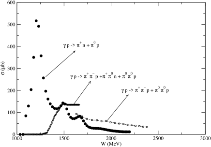
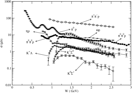
Figure 1: The total cross section data of meson production in $\gamma p$ reaction. Left: $1-\pi$ and $2-\pi$ production are compared. Right: KY ( $K^{+}\Lambda$, $K^{+}\Sigma^{0}$, $K^{0}\Sigma^{+}$), $\eta p$, and $\omega p$ production are compared with some of the $1-\pi$ and $2-\pi$ production

The main challenge of developing dynamical reaction models of meson production reactions in the $N^{*}$ region can be seen in Fig.1. We see that two-pion photo-production cross sections shown in the left-hand-side become larger than the one-pion photo-production as the $\gamma p$ invariant mass exceeds $W\sim 1.4$ GeV. In the right-hand-side, KY ( $K^{+}\Lambda$, $K^{+}\Sigma^{0}$, $K^{0}\Sigma^{+}$), $\eta p$, and $\omega p$ production cross sections are a factor of about 10 weaker than the dominant $\pi^{+}\pi^{-}p$ production. From the unitarity condition, we have for any single meson production process $\gamma N\rightarrow MB$ with $MB=\pi N,\eta N,\omega N,K\Lambda,K\Sigma$

$$i(T_{\gamma N,MB}-T^{*}_{MB,\gamma N}) = \sum_{M^{\prime}B^{\prime}}T_{\gamma N,M^{\prime}B^{\prime}}\rho_{M^{\prime}B^{\prime}}T^{*}_{MB,M^{\prime}B^{\prime}}$$ (1)

$$+T_{\gamma N,\pi\pi N}\rho_{\pi\pi N}T^{*}_{MB,\pi\pi N}\,,$$

where $\rho_{\alpha}$ denotes an appropriate phase space factor for the channel $\alpha$. The large two-pion production cross sections seen in Fig.1 indicate that the second term in the right-hand-side of Eq.(1) is significant and hence the single meson production reactions above the $\Delta$ region must be influenced strongly by the coupling with the two-pion channels. Similarly, the two-pion production $\gamma N\rightarrow\pi\pi N$ is also influenced by the transition to two-body $MB$ channel

$$i(T_{\gamma N,\pi\pi N}-T^{*}_{\pi\pi N,\gamma N}) = \sum_{M^{\prime}B^{\prime}}T_{\gamma N,M^{\prime}B^{\prime}}\rho_{M^{\prime}B^{\prime}}T^{*}_{\pi\pi N,M^{\prime}B^{\prime}}$$ (2)

$$+T_{\gamma N,\pi\pi N}\rho_{\pi\pi N}T^{*}_{\pi\pi N,\pi\pi N}\,.$$

Clearly, a sound dynamical reaction model must be able to describe the two pion production and to account for the above unitarity conditions.

The development of meson-baryon reaction models including two-pion production channel has a long history. It was already recognized in 1960’s, as discussed by Blankenbecler and Sugarbs , that the dispersion-relation approach, which has been very successful in analyzing the data of $\pi N$ elastic scatteringhohler and $\gamma N\rightarrow\pi N$ reactionscgln ; donnachie , can not be used to analyze the data of two-pion production. The reason is that apart from the $\pi N$ and $\pi\pi N$ unitarity cuts, it is rather impossible to even guess the analytic structure of two-pion production amplitudes. Furthermore, the dispersion relation models are difficult to solve because of their bi-linear structure which is the price of only dealing with the on-shell amplitudes.

Ideally, one would like to find alternatives to analyze the $\pi N$ and $\gamma N$ reaction data completely within the framework of relativistic quantum field theory. The Bethe-Salpeter (BS) equation has been taken historically as the starting point of such an ambitious approach. The complications involved in solving the BS equation have been known for long time. For example, its singularity structure and the associated numerical problems were very well discussed in Refs.tjon-1 ; tjon-2 ; afnan-1 . The BS equation contains serious singularities arising from the pinching of the integration over the time component. In addition to the two-body unitarity cut, it has a selected set of n-body unitarity cuts, as explained in great detail in Ref.afnan-1 . Considerable numerical efforts are already needed to solve the Ladder BS equation for $\pi N$ elastic scattering, as can be seen in the work of Lahiff and Afnanafnan-2 . Using the Wick rotation, they can solve the Ladder BS equation below two-pion production threshold with very restricted choices of form factors. It is not clear how to extend their work to higher energies.

The first main progress in finding an alternative to the dispersion-relation approach was perhaps also made by Blankenbecler and Sugarbs . By imposing the unitarity condition, they show that the Bethe-Salpeter equation can be reduced into a covariant three-dimensional equation which is linear and can be managed in practice. Compared with the dispersion relation approach, the challenge here is account for the off-shell dynamics. This approach was later further developed by Aaron, Amado, and Young (AAY)aay . With the assumption that all interactions are due to the formation and decay of isobars, they developed a set of covariant three-dimensional equations for describing both the $\pi N$ elastic scattering and $\pi N\rightarrow\pi\pi N$ reaction. They however had only obtainedaay ; aay-1 ; aa-1 ; aa-2 a very qualitative description of the $\pi N$ data and only investigated very briefly the electromagnetic meson production reactions. Their results suggested the limitation of the isobar model and the need of additional mechanisms. For example, the $N^{*}$ excitation mechanisms are not included in their formulation. They then proposedaa-76 an approach to include the additional mechanisms phenomenologically in fitting the data by using the ”minimal” equations which are rigorously constrained by the $\pi N$ and $\pi\pi N$ unitarity conditions and have the correct analyticity of the isobar model. The AAY approach was later applied mainly in the studies of $\pi NN$ systems, such as those by Afnan and Thomasafnan-thomas and by Matsuyama and Yazakimatsuyama . Development in this direction was well reviewed in Ref.garcilazo .

The dynamical study of $\pi N$ scattering was pursued further in 1980’s by Pearce and Afnanpa-86 ; ap-87 ; afnan-88 . They derived the $\pi N$ scattering equations by using a diagrammatic method, originally developed for investigating the $\pi NN$ problemgarcilazo , to sum the perturbation diagrams which are selected by imposing the unitarity condition. Furthermore, they relate the $\pi N$ scattering to the cloudy bag model by extending the work of Thieberg, Thomas and Millercbm-1 ; cbm-2 ; cbm-3 to include the $\pi\pi N$ unitarity condition.

Since 1990 the $\pi N$ and $\gamma N$ reactions have been investigated mainly by using either the three-dimensional reductionsklein of the Bethe-Salpeter equation or the unitary transformation methodssl-1 ; fuda-1 . These efforts were motivated mainly by the success of the meson-exchange models of $NN$ scatteringmachleidt , and have yielded the meson-exchange models developed by Pearce and Jenningspj-91 , National Taiwan University-Argonne National Laboratory (NTU-ANL) collaboration ntuanl-1 ; ntuanl-2 , Gross and Suryagross , Sato and Leesl-1 ; sl-2 , Julich Groupjulich-1 ; julich-2 ; julich-3 ; julich-4 , Fuda and his collaboratorsfuda-1 ; fuda-2 , and Utretch-Ohio collaborationpasc-1 ; pasc-2 . All of these dynamical models can describe well the data in the $\Delta$ region, but have not been fully developed in the higher mass $N^{*}$ region. The main challenge is to include correctly the coupling with the $\pi\pi N$ channels.

We now return to discussing the two-pion production channel which is an essential part of our formulation. Most of the recent two-pion production calculations are the extensions of the isobar model of Lüke and Södingluke . The production mechanisms are calculated from tree-diagrams of appropriately chosen Lagrangians. The calculations of Valencia Grouposet included the tree diagrams calculated from Lagrangians with $\gamma$, $N$, $\pi$, $\rho$, $\Delta$(1232), $N^{*}(1440)$, and $N^{*}(1520)$ fields. To describe the total cross section data in all charged $\pi\pi N$ channels, they also includedoset-1 the production of $\Delta(1700)$ and $\rho$ effect arising from $N^{*}(1520)$.

The model developed by Ochi, Hirata, Katagiri, and Takakihirata-1 ; hirata-2 ; hirata-3 contains the tree diagrams calculated from Lagrangians with $\gamma$, $\pi$, $\rho$, $\omega$, $N$, $\Delta$ and $N^{*}(1520)$ fields. An important feature of this model is to describe the excitation of $N^{*}(1520)$ within an isobar model with three channels $\pi N$, $\rho N$, and $\pi\Delta$. They found that the invariant mass distributions of all charged channels of $\gamma p\rightarrow\pi\pi N$ can be better described if the pseudo-scalar $\pi NN$ coupling is used. They also found that the $N^{*}(1520)\rightarrow\rho N$ decay is the essential mechanism to explain the differences between the invariant mass distributions of $\pi^{+}\pi^{0}$ and $\pi^{0}\pi^{0}$. Similar tree-diagram calculations of two pion photo-production have also been performed by Murphy and Lagetlaget .

The analysesmokeev-1 ; mokeev-2 ; mokeev-3 of two pion production by using the JLab-Moscow State University (JLAB-MSU) isobar model considered only the minimum set of the tree diagrams proposed in the original work of Lüke and Södingluke . However, they made two improvements. They included all 3-star and 4-star resonances listed by the Particle Data Group and used the absorptive model developed by Gottfried and Jacksongott to account for the initial and final state interactions. They found that the $\pi N\Delta$ form factor is needed to get agreement with the data of $\gamma p\rightarrow\pi^{-}\Delta^{++}$, while the initial and final state interactions are not so large. In analyzing the two-pion electro-production data, they further included a $\pi\pi N$ phase-space term with its magnitude adjusted to fit the data. This term was later replaced by a phenomenological particle-exchange amplitude which improves significantly the fits to the data. With this model, they had identifiedmokeev-3 a new $N^{*}$($\frac{3}{2}^{+},1720$) and the production of the isobar channel $\pi^{+}D_{13}(1520)$ which has never been considered before.

The common feature of all of the two-pion production calculations described above is that the coupled-channel effects due to the unitarity condition, such as that given in Eqs.(1)-(2), are not included. The problems arise from this simplification were very well studied by Aaron and Amadoaa-76 , and will be discussed later in this paper. While the results from these tree-diagram models are very useful for identifying the reaction mechanisms, their findings concerning $N^{*}$ properties must be further examined. To make progress, it is necessary to develop a coupled-channel formulation within which the $\pi\pi N$ channel is explicitly included. In this paper, we report our effort in this direction.

We have developed a dynamical coupled-channel model by extending the model developed in Refs.sl-1 ; sl-2 to include the higher mass $N^{*}$ and all relevant reaction channels seen in Fig.1. Our presentations will only include two-particle channels $MB=\gamma N$, $\pi N$, $\eta N$ and three-particle channel $\pi\pi N$ which has resonant components $\pi\Delta$, $\rho N$, and $\sigma N$. But the formulation can be easily extended to include other two-particle channels such as $\omega N$, $K\Lambda$ and $K\Sigma$ and three-particle channels such as $\pi\eta N$ and $K\bar{K}N$.

Our main purpose here is to give a complete and detailed presentation of our model and the numerical methods needed to solve the resulting coupled-channel equations. A complete coupled-channel analysis requires a simultaneous fit to all of the meson production data from $\pi N$ and $\gamma N$ reactions, such as the total cross section data illustrated in Fig.1 and the very extensive data from recent high precision experiments on photo-production and electro-production reactions. Obviously, this is a rather complex problem which can not be accomplished in this paper. Instead, we will apply our approach only to address the theoretical questions concerning the effects due to $\pi\pi N$ unitarity cuts. For this very limited purpose, we present results from our first calculations of $\gamma N\rightarrow\pi\pi N$ reactions.

In section II, we present the model Hamiltonian of our formulation. It is derived from a set of Lagrangians, given explicitly in Appendix A, by applying the unitary transformation method which was explained in detail in Refs.sl-1 ; sko . The coupled-channel equations are then derived from the model Hamiltonian in section III with details explained in Appendix B. In section IV, we explain the procedures for performing numerical calculations within our formulation. The numerical methods for solving the coupled-channel equations with $\pi\pi N$ cut are explained in section V. Results of $\gamma p\rightarrow\pi\pi N$ are presented and discussed in section VI. A summary and the plans for future developments are given in section VII. For the completeness in explaining our numerical procedures, several appendices are given to present explicitly the formula for efficient calculations of a very large number of partial-wave matrix elements which are the input to the coupled-channel equations, and to explain how the constructed resonant amplitudes are related to the information listed by the Particle Data Group (PDG)pdg .

II Model Hamiltonian

In this section we present a model Hamiltonian for constructing a coupled-channel reaction model with $\gamma N$, $\pi N$, $\eta N$ and $\pi\pi N$ channels. Since significant parts of the $\pi\pi N$ production are known experimentally to be through the unstable states $\pi\Delta$, $\rho N$, and perhaps also $\sigma N$, we will also include $bare$ $\Delta$, $\rho$ and $\sigma$ degrees of freedom in our formulation. Furthermore, we introduce $bare$ $N^{*}$ states to represent the quark-core components of the nucleon resonances. The model is expected to be valid up to $W=2$ GeV below which three pion production is very weak.

Similar to the model of Refs.sl-1 ; sl-2 (commonly called the SL model), our starting point is a set of Lagrangians describing the interactions between mesons ($M=\gamma,\pi,\eta,\rho,\omega,\sigma\cdot\cdot\cdot$) and baryons ($B=N,\Delta,N^{*}\cdot\cdot\cdot$). These Lagrangian are constrained by various well-established symmetry properties, such as the invariance under isospin, parity, and gauge transformation. The chiral symmetry is also implemented as much as we can. The considered Lagrangians are given in Appendix A. By applying the standard canonical quantization, we obtain a Hamiltonian of the following form

$$H = \int{\it h(\vec{x},t=0)}d\vec{x}$$ (3)

$$= H_{0}+H_{I}\,,$$

where ${\it h(\vec{x},t)}$ is the Hamiltonian density constructed from the starting Lagrangians and the conjugate momentum field operators. In Eq.(3), $H_{0}$ is the free Hamiltonian and

$$H_{I}=\sum_{M,B,B^{\prime}}\Gamma_{MB\leftrightarrow B^{\prime}}+\sum_{M,M^{\prime},M^{\prime\prime}}h_{M^{\prime}M^{\prime\prime}\leftrightarrow M}\,,$$ (4)

where $\Gamma_{MB\leftrightarrow B^{\prime}}$ describes the absorption and emission of a meson($M$) by a baryon($B$) such as $\pi N\leftrightarrow N$ and $\pi N\leftrightarrow\Delta$, and $h_{M^{\prime}M^{\prime\prime}\leftrightarrow M}$ describes the vertex interactions between mesons such as $\pi\pi\leftrightarrow\rho$ and $\gamma\pi\leftrightarrow\pi$. Clearly, it is a non-trivial many body problem to calculate meson-baryon scattering and meson production reaction amplitudes from the Hamiltonian defined by Eqs.(3)-(4). To obtain a manageable reaction model, we apply a unitary transformation methodsl-1 ; sko to derive an effective Hamiltonian from Eqs.(3)-(4). The essential idea of the employed unitary transformation method is to eliminate the unphysical vertex interactions $MB\rightarrow B^{\prime}$ with masses $m_{M}+m_{B}<m_{B^{\prime}}$ from the Hamiltonian and absorb their effects into $MB\rightarrow M^{\prime}B^{\prime}$ two-body interactions. The resulting effective Hamiltonian is energy independent and hence is easy to be used in developing reaction models and performing many-particle calculations. The details of this method have been explained in section II and the appendix of Ref.sl-1 .

Our main step is to derive from Eqs.(3)-(4) an effective Hamiltonian which contains interactions involving $\pi\pi N$ three-particle states. This is accomplished by applying the unitary transformation method up to the third order in interaction $H_{I}$ of Eq.(4). The resulting effective Hamiltonian is of the following form

$$H_{eff}=H_{0}+V\,,$$ (5)

with

$$H_{0}=\sum_{\alpha}K_{\alpha}\,,$$ (6)

where $K_{\alpha}=\sqrt{m_{\alpha}^{2}+\vec{p_{\alpha}}^{2}}$ is the free energy operator of particle $\alpha$ with a mass $m_{\alpha}$, and the interaction Hamiltonian is

$$V=\Gamma_{V}+v_{22}+v^{\prime}\,,$$ (7)

where

$$\Gamma_{V} = \{\sum_{N^{*}}(\sum_{MB}\Gamma_{N^{*}\rightarrow MB}+\Gamma_{N^{*}\rightarrow\pi\pi N})+\sum_{M^{*}}h_{M^{*}\rightarrow\pi\pi}\}+\{c.c.\}\,,$$ (8)

$$v_{22} = \sum_{MB,M^{\prime}B^{\prime}}v_{MB,M^{\prime}B^{\prime}}+v_{\pi\pi}\,.$$ (9)

Here ${c.c.}$ denotes the complex conjugate of the terms on its left-hand-side. In the above equations, $MB=\gamma N,\pi N,\eta N,\pi\Delta,\rho N,\sigma N$ represent the considered meson-baryon states. The resonance associated with the $bare$ baryon state $N^{*}$ is induced by the vertex interactions $\Gamma_{N^{*}\rightarrow MB}$ and $\Gamma_{N^{*}\rightarrow\pi\pi N}$. Similarly, the $bare$ meson states $M^{*}$ = $\rho$, $\sigma$ can develop into resonances through the vertex interaction $h_{M^{*}\rightarrow\pi\pi}$. These vertex interactions are illustrated in Fig.2(a). Note that the masses $M^{0}_{N^{*}}$ and $m^{0}_{M^{*}}$ of the bare states $N^{*}$ and $M^{*}$ are the parameters of the model which will be determined by fitting the $\pi N$ and $\pi\pi$ scattering data. They differ from the empirically determined resonance positions by mass shifts which are due to the coupling of the bare states with the meson-baryon $scattering$ states. It is thus reasonable to speculate that these bare masses can be identified with the mass spectrum predicted by the hadron structure calculations which do not account for the meson-baryon $continuum$ scattering states, such as the calculations based on the constituent quark models which do not have meson-exchange quark-quark interactions. It is however much more difficult, but more interesting, to relate these bare masses to the $current$ Lattice QCD calculations which can not account for the scattering states rigorously mainly because of the limitation of the lattice spacing.

In Eq.(9), $v_{MB,M^{\prime}B^{\prime}}$ is the non-resonant meson-baryon interaction and $v_{\pi\pi}$ is the non-resonant $\pi\pi$ interaction. They are illustrated in Fig.2(b). The third term in Eq.(7) describes the non-resonant interactions involving $\pi\pi N$ states

$$v^{\prime}=v_{23}+v_{33}$$ (10)

with

$$v_{23} = \sum_{MB}[(v_{MB,\pi\pi N})+(c.c.)]$$

$$v_{33} = v_{\pi\pi N,\pi\pi N}\,.$$

They are illustrated in Fig.2(c). All of these interactions are defined by the tree-diagrams generated from the considered Lagrangians. They are illustrated in Fig.3 for two-body interactions $v_{MB,M^{\prime}B^{\prime}}$ and in Fig.4 for $v_{MB,\pi\pi N}$. Some leading mechanisms of $v_{\pi\pi}$ and $v_{\pi\pi N,\pi\pi N}$ are illustrated in Fig.5. The calculations of the matrix elements of these interactions will be discussed later in the section on our calculations and detailed in appendices. Here we only mention that the matrix elements of these interactions are calculated from the usual Feynman amplitudes with their time components in the propagators of intermediate states defined by the three momenta of the initial and final states, as specified by the unitary transformation methods. Thus they are independent of the collision energy $E$.

Figure 2: Basic mechanisms of the Model Hamiltonian defined in Eqs.(8)-(10).

Figure 3: Mechanisms for $v_{MB,M^{\prime}B^{\prime}}$ of Eq.(9): (a) direct s-channel, (b) crossed u-channel, (c) one-particle-exchange t-channel, (d) contact interactions.

Figure 4: Examples of non-resonant mechanisms of $v_{MN,\pi\pi N}$ with $M=\pi$ or $\gamma$ (denoted by long-dashed lines). $M_{I}$ denotes the intermediate mesons ($\pi,\rho,\omega$).

Figure 5: Examples of non-resonant mechanisms of $v_{\pi\pi}$ and $v_{\pi\pi N,\pi\pi N}$

III Dynamical Coupled-Channel Equations

With the Hamiltonian defined by Eqs.(5)-(10) , we follow the formulation of Ref.gw to define the scattering S-matrix as

$$S_{ab}(E)=\delta_{ab}-(2\pi)iT_{ab}(E)\,,$$ (11)

where the scattering T-matrix is defined by

$$T_{ab}(E)=<a|T(E)|b>$$

with

$$T(E)=V+V\frac{1}{E-H_{0}+i\epsilon}T(E)\,.$$ (12)

Since the interaction $V$, defined by Eqs.(7)-(10), is energy independent, it is rather straightforward to follow the formal scattering theory given in Ref.gw to show that Eq.(12) leads to the following unitarity condition

$$(T(E)-T^{\dagger}(E))_{ab}=-2\pi i\sum_{c}T^{\dagger}_{ac}(E)\delta(E_{c}-E)T_{cb}(E)\,,$$ (13)

where $a,b,c$ are the reaction channels in the considered energy region.

Our task is to derive from Eq.(12) a set of dynamical coupled-channel equations for practical calculations within the model space $N^{*}\oplus MB\oplus\pi\pi N$. In the derivations, the unitarity condition Eq.(13) must be maintained exactly. We achieve this rather complex task by applying the standard projection operator techniquesfeshbach , similar to that employed in a studyLM85 of $\pi NN$ scattering. The details of our derivations are given in Appendix B. To explain our coupled-channel equations, it is sufficient to present the formula obtained from setting $\Gamma_{N^{*}\rightarrow\pi\pi N}=0$ in our derivations. The resulting model is defined by Eqs.(B74)-(B96) of appendix B. Here we explain these equations and discuss their dynamical content.

The resulting $MB\rightarrow M^{\prime}B^{\prime}$ amplitude $T_{MB\rightarrow M^{\prime}B^{\prime}}$ in each partial wave is illustrated in Fig.6. It can be written as

$$T_{MB,M^{\prime}B^{\prime}}(E) = t_{MB,M^{\prime}B^{\prime}}(E)+t^{R}_{MB,M^{\prime}B^{\prime}}(E)\,,$$ (14)

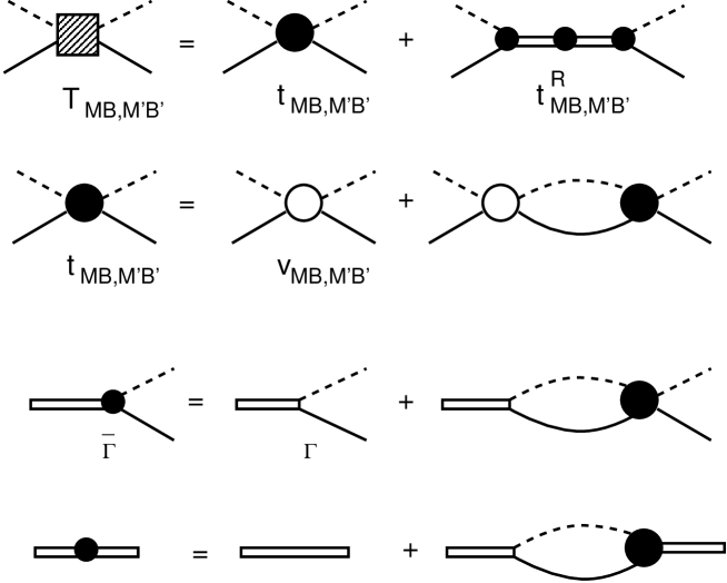
Figure 6: Graphical representations of Eqs.(14)-(19).

The second term in the right-hand-side of Eq.(14) is the resonant term defined by

$$t^{R}_{MB,M^{\prime}B^{\prime}}(E)=\sum_{N^{*}_{i},N^{*}_{j}}\bar{\Gamma}_{MB\rightarrow N^{*}_{i}}(E)[D(E)]_{i,j}\bar{\Gamma}_{N^{*}_{j}\rightarrow M^{\prime}B^{\prime}}(E)\,,$$ (15)

with

$$[D(E)^{-1}]_{i,j}(E)=(E-M^{0}_{N^{*}_{i}})\delta_{i,j}-\bar{\Sigma}_{i,j}(E)\,,$$ (16)

where $M_{N^{*}}^{0}$ is the bare mass of the resonant state $N^{*}$, and the self-energies are

$$\bar{\Sigma}_{i,j}(E)=\sum_{MB}\Gamma_{N^{*}_{i}\rightarrow MB}G_{MB}(E)\bar{\Gamma}_{MB\rightarrow N^{*}_{j}}(E)\,.$$ (17)

The dressed vertex interactions in Eq.(15) and Eq.(17) are (defining $\Gamma_{MB\rightarrow N^{*}}=\Gamma^{\dagger}_{N^{*}\rightarrow MB}$)

$$\bar{\Gamma}_{MB\rightarrow N^{*}}(E) = {\Gamma_{MB\rightarrow N^{*}}}+\sum_{M^{\prime}B^{\prime}}t_{MB,M^{\prime}B^{\prime}}(E)G_{M^{\prime}B^{\prime}}(E)\Gamma_{M^{\prime}B^{\prime}\rightarrow N^{*}}\,,$$ (18)

$$\bar{\Gamma}_{N^{*}\rightarrow MB}(E) = \Gamma_{N^{*}\rightarrow MB}+\sum_{M^{\prime}B^{\prime}}\Gamma_{N^{*}\rightarrow M^{\prime}B^{\prime}}G_{M^{\prime}B^{\prime}}(E)t_{M^{\prime}B^{\prime},MB}(E)\,.$$ (19)

The meson-baryon propagator $G_{MB}$ in the above equations takes the following form

$$G_{MB}(E)=\frac{1}{E-K_{B}-K_{M}-\Sigma_{MB}(E)+i\epsilon}\,,$$ (20)

where the mass shift $\Sigma_{MB}(E)$ depends on the considered $MB$ channel. It is $\Sigma_{MB}(E)=0$ for the stable particle channels $MB=\pi N,\eta N$. For channels containing an unstable particle, such as $MB=\pi\Delta,\rho N,\sigma N$, we have

$$\Sigma_{MB}(E)=[<MB|g_{V}\frac{P_{\pi\pi N}}{E-K_{\pi}-K_{\pi}-K_{N}+i\epsilon}g^{\dagger}_{V}|MB>]_{un-connected}$$ (21)

with

$$g_{V}=\Gamma_{\Delta\rightarrow\pi N}+h_{\rho\rightarrow\pi\pi}+h_{\sigma\rightarrow\pi\pi}\,.$$ (22)

In Eq.(21) ”$un-connected$” means that the stable particle, $\pi$ or $N$, of the $MB$ state is a spectator in the $\pi\pi N$ propagation. Thus $\Sigma_{MB}(E)$ is just the mass renormalization of the unstable particle in the $MB$ state.

It is important to note that the resonant amplitude $t^{R}_{M^{\prime}B^{\prime},MB}(E)$ is influenced by the non-resonant amplitude $t_{M^{\prime}B^{\prime},MB}(E)$, as seen in Eq.(15)-(19). In particular, Eqs.(18)-(19) describe the meson cloud effects on $N^{*}$ decays, as illustrated in Fig.7 for the $\Delta\rightarrow\gamma N$ decay interpreted in Refs.sl-1 ; sl-2 . This feature of our formulation is essential in interpreting the extracted resonance parameters.

Figure 7: Graphical representation of the dressed $\bar{\Gamma}_{\Delta,\gamma N}$ interpreted in Refs.sl-1 ; sl-2 .

Here we note that the $N^{*}$ propagator $D(E)$ defined by Eq.(16) can be diagonalized to write the resonant term Eq.(15) as

$$t^{R}_{MB,M^{\prime}B^{\prime}}(k,k^{\prime})=\sum_{\bar{N}^{*}}\frac{\tilde{\Gamma}_{MB\rightarrow\bar{N}^{*}}(k)\tilde{\Gamma}_{\bar{N}^{*}\rightarrow M^{\prime}B^{\prime}}(k^{\prime})}{E-{M}_{\bar{N}^{*}}(E)+\frac{i}{2}\Gamma^{tot}_{\bar{N}^{*}}(E)}\,,$$ (23)

where $\tilde{\Gamma}_{MB\rightarrow\bar{N^{*}}}$ and mass parameters ${M}_{\bar{N}^{*}}(E)$ and $\Gamma^{tot}_{\bar{N^{*}}}(E)$ are of course related the dressed vertexes $\bar{\Gamma}_{N^{*}\rightarrow MB}$ and self energies $\Sigma_{i,j}$ defined in Eqs.(17)-(19). Eq.(23) is similar to the usual Breit-Wigner form and hence can be used to relate our model to the empirical resonant parameters listed by Particle Data Group. This non-trivial subject is being investigated in Ref. suzuki .

The non-resonant amplitudes $t_{MB,M^{\prime}B^{\prime}}$ in Eq.(14) and Eqs.(18)-(19) are defined by the following coupled-channel equations

$$t_{MB,M^{\prime},B^{\prime}}(E) = V_{MB,M^{\prime}B^{\prime}}(E)+\sum_{M^{\prime\prime}B^{\prime\prime}}V_{MB,M^{\prime\prime}B^{\prime\prime}}(E)G_{M^{\prime\prime}B^{\prime\prime}}(E)t_{M^{\prime\prime}B^{\prime\prime},M^{\prime}B^{\prime}}(E)$$ (24)

with

$$V_{MB,M^{\prime}B^{\prime}}(E)=v_{MB,M^{\prime}B^{\prime}}+Z_{{M}{B},{M}^{\prime}{B}^{\prime}}(E)\,.$$ (25)

Here $Z_{{M}{B},{M}^{\prime}{B}^{\prime}}(E)$ contains the effects due to the coupling with $\pi\pi N$ states. It has the following form

$$Z_{{M}{B},{M}^{\prime}{B}^{\prime}}(E) = <{M}{B}\mid F\frac{P_{\pi\pi N}}{E-H_{0}-\hat{v}_{\pi\pi N}+i\epsilon}F^{\dagger}\mid{M}^{\prime}{B}^{\prime}>$$ (26)

$$-[\delta_{MB,M^{\prime}B^{\prime}}\Sigma_{MB}(E)]$$

with

$$\hat{v}_{\pi\pi N} = v_{\pi N,\pi N}+v_{\pi\pi}+v_{\pi\pi N,\pi\pi N}\,,$$ (27)

$$F = g_{V}+v_{MB,\pi\pi N}\,,$$ (28)

where $g_{V}$ has been defined in Eq.(22). Note that the second term in Eq.(26) is the effect which is already included in the mass shifts $\Sigma_{MB}$ of the propagator Eq.(20) and must be removed to avoid double counting.

The appearance of the projection operator $P_{\pi\pi N}$ in Eqs.(21) and (26) is the consequence of the unitarity condition Eq.(13). To isolate the effects entirely due to the vertex interaction $g_{V}=\Gamma_{\Delta\rightarrow\pi N}+h_{\rho\rightarrow\pi\pi}+h_{\sigma\rightarrow\pi\pi}$, we use the operator relation Eq.(B33) of Appendix B to decompose the $\pi\pi N$ propagator of Eq.(26) to write

$$Z_{MB,M^{\prime}B^{\prime}}(E)=Z^{(E)}_{MB,M^{\prime}B^{\prime}}(E)+Z^{(I)}_{MB,M^{\prime}B^{\prime}}(E)\,.$$ (29)

The first term is

$$Z^{(E)}_{MB,M^{\prime}B^{\prime}}(E) = <MB\mid g_{V}\frac{P_{\pi\pi N}}{E-H_{0}+i\epsilon}g^{\dagger}_{V}\mid M^{\prime}B^{\prime}>-[\delta_{MB,M^{\prime}B^{\prime}}\Sigma_{MB}(E)]\,.$$ (30)

Obviously, $Z^{(E)}_{MB,M^{\prime}B^{\prime}}(E)$ is the one-particle-exchange interaction between unstable particle channels $\pi\Delta$, $\rho N$, and $\sigma N$, as illustrated in Fig.8. The second term of Eq.(29) is

$$Z^{(I)}_{MB,M^{\prime}B^{\prime}}(E) = <MB\mid F\frac{P_{\pi\pi N}}{E-H_{0}+i\epsilon}t_{\pi\pi N,\pi\pi N}(E)\frac{P_{\pi\pi N}}{E-H_{0}+i\epsilon}F^{\dagger}\mid M^{\prime}B^{\prime}>$$ (31)

$$+<MB\mid g_{V}\frac{P_{\pi\pi N}}{E-H_{0}+i\epsilon}v^{\dagger}_{MB,\pi\pi N}\mid B^{\prime}M^{\prime}>$$

$$+<MB\mid v_{MB,\pi\pi N}\frac{P_{\pi\pi N}}{E-H_{0}+i\epsilon}g^{\dagger}_{V}\mid M^{\prime}B^{\prime}>$$

$$+<MB\mid v_{MB,\pi\pi N}\frac{P_{\pi\pi N}}{E-H_{0}+i\epsilon}v^{\dagger}_{MB,\pi\pi N}\mid M^{\prime}B^{\prime}>\,.$$

Some of the leading terms of $Z^{(I)}_{MB,M^{\prime}B^{\prime}}(E)$ are illustrated in Fig.9. Here $t_{\pi\pi N,\pi\pi N}(E)$ is a three-body scattering amplitude defined by

$$t_{\pi\pi N,\pi\pi N}(E)=\hat{v}_{\pi\pi N}+\hat{v}_{\pi\pi N}\frac{1}{E-K_{\pi}-K_{\pi}-K_{N}-\hat{v}_{\pi\pi N}+i\epsilon}\hat{v}_{\pi\pi N}$$ (32)

where $\hat{v}_{\pi\pi N}$ has been defined in Eq.(27). Few leading terms of Eq.(32) due to the direct s-channel interaction $v^{s}$ (illustrated in Fig.3) of $v_{\pi N,\pi N}$ are shown in Fig.10. These terms involve the $\pi\pi N$ propagator ${1}/({E-K_{\pi}-K_{\pi}-K_{N}+i\epsilon})$ and obviously can generate $\pi\pi N$ cut effects which are due to the $\pi\pi N$ vertex. This observation indicates that the $\pi N$ scattering equation of Aaron, Amado, and Youngaay can be related to our formulation if the interactions which are $only$ determined by the $\pi\pi N$ vertex are kept in the equations presented above. We however will not discuss this issue in this paper. The relations between our formulation and the $AAY$ model can be better understood in our next publicationjlms where we will determine the strong interaction parts of our Hamiltonian by fitting $\pi N$ reaction data up to invariant mass $W=2$ GeV.

Figure 8: One-particle-exchange interactions $Z^{(E)}_{\pi\Delta,\pi\Delta}(E)$, $Z^{(E)}_{\rho N,\pi\Delta}$ and $Z^{(E)}_{\sigma N,\pi\Delta}$ of Eq.(30).

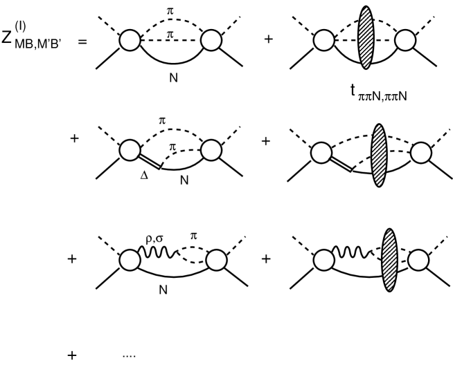
Figure 9: Examples of mechanisms included in $Z^{(I)}_{MB,M^{\prime}B^{\prime}}(E)$ of Eq.(31).

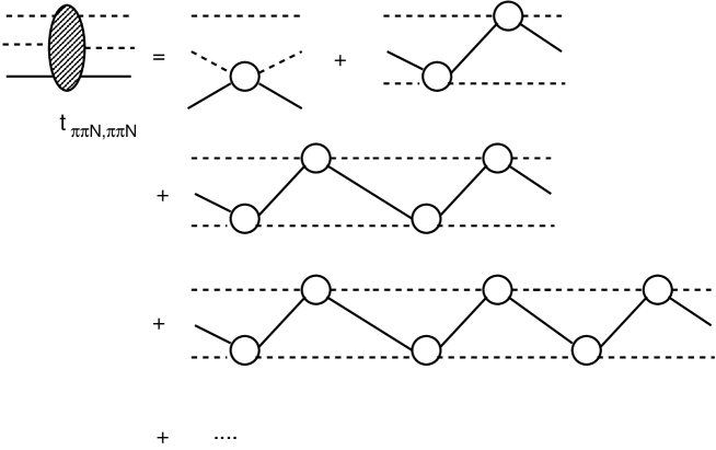
Figure 10: Some of the leading order terms of $t_{\pi\pi N,\pi\pi N}$ of Eq.(32). The open circle represents the direct s-channel interaction $v^{s}$ illustrated in Fig.3 for the $MB=M^{\prime}B^{\prime}=\pi N$ case.

The amplitudes $T_{MB,M^{\prime}B^{\prime}}=t_{MB,M^{\prime}B^{\prime}}+t^{R}_{MB,M^{\prime}B^{\prime}}$ defined by Eq.(14) can be used directly to calculate the cross sections of $\pi N\rightarrow\pi N,\eta N$ and $\gamma N\rightarrow\pi N,\eta N$ reactions. They are also the input to the calculations of the two-pion production amplitudes. The two-pion production amplitudes resulted from our derivations given in Appendix B are illustrated in Fig.11. They can be cast exactly into the following form

$$T_{\pi\pi N,MB}(E)=T^{dir}_{\pi\pi N,MB}(E)+T^{\pi\Delta}_{\pi\pi N,MB}(E)+T^{\rho N}_{\pi\pi N,MB}(E)+T^{\sigma N}_{\pi\pi N,MB}(E)$$ (33)

with

$$T^{dir}_{\pi\pi N,MB}(E) = <\psi^{(-)}_{\pi\pi N}(E)|\sum_{M^{\prime}B^{\prime}}v_{\pi\pi N,M^{\prime}B^{\prime}}[\delta_{M^{\prime}B^{\prime},MB}$$ (34)

$$+G_{M^{\prime}B^{\prime}}(E)(t_{M^{\prime}B^{\prime},MB}(E)+t^{R}_{M^{\prime}B^{\prime},MB})]|MB>\,,$$

$$T^{\pi\Delta}_{\pi\pi N,MB}(E) = <\psi^{(-)}_{\pi\pi N}(E)|\Gamma^{\dagger}_{\Delta\rightarrow\pi N}G_{\pi\Delta}(E)[t_{\pi\Delta,MB}(E)+t^{R}_{\pi\Delta,MB}(E)]|MB>\,,$$ (35)

$$T^{\rho N}_{\pi\pi N,MB}(E) = <\psi^{(-)}_{\pi\pi N}(E)|h^{\dagger}_{\rho\rightarrow\pi\pi}G_{\rho N}(E)[t_{\rho N,MB}(E)+t^{R}_{\rho N,MB}(E)]|MB>\,,$$ (36)

$$T^{\sigma N}_{\pi\pi N,MB}(E) = <\psi^{(-)}_{\pi\pi N}(E)|h^{\dagger}_{\sigma\rightarrow\pi\pi}G_{\sigma N}(E)[t_{\sigma N,MB}(E)+t^{R}_{\sigma N,MB}(E)]|MB>\,.$$ (37)

In the above equations, the $\pi\pi N$ scattering wave function is defined by

$$<\psi^{(-)}_{\pi\pi N}(E)| = <\pi\pi N|\Omega^{(-)\dagger}_{\pi\pi N}(E)\,,$$ (38)

where the scattering operator is defined by

$$\Omega^{(-)\dagger}_{\pi\pi N}(E)=<\pi\pi N|[1+t_{\pi\pi N,\pi\pi N}(E)\frac{1}{E-K_{\pi}-K_{\pi}-K_{N}+i\epsilon}]\,.$$ (39)

Here the three-body scattering amplitude $t_{\pi\pi N,\pi\pi N}(E)$ is determined by the non-resonant interactions $v_{\pi\pi}$, $v_{\pi N,\pi N}$ and $v_{\pi\pi N,\pi\pi N}$, as defined by Eq.(32).

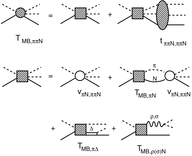
Figure 11: Graphical representations of $T_{\pi\pi N,MB}$ defined by Eqs.(33)-(37).

We note here that the direct production amplitude $T^{dir}_{\pi\pi N,MB}(E)$ of Eq.(34) is due to $v_{\pi\pi N,MB}$ interaction illustrated in Fig.4, while the other three terms are through the unstable $\pi\Delta$, $\rho N$, and $\sigma N$ states. Each term has the contributions from the non-resonant amplitude $t_{M^{\prime}B^{\prime},MB}(E)$ and resonant term $t^{R}_{M^{\prime}B^{\prime},MB}(E)$. As seen in Eq.(15)-(19), the resonant amplitude $t^{R}_{M^{\prime}B^{\prime},MB}(E)$ is influenced by the non-resonant amplitude $t_{M^{\prime}B^{\prime},MB}(E)$. This an important consequence of unitarity condition Eq.(13).

IV Calculations

The $N^{*}$ information can be accurately extracted only when the extensive meson production data of $\pi N$ and $\gamma N$ reactions are analyzed simultaneously. Obviously, this is a rather complex task by using the dynamical coupled-channel formulation described in section III. In addition, it is a highly non-trivial numerical task to solve the coupled-channel equation Eq.(24) which contains a logarithmically divergent driving term $Z_{MB,M^{\prime}B^{\prime}}{(E)}$ defined by Eqs.(29)-(31). As a first step, we focus in this work on the development of numerical methods for solving this coupled-channel equation. This then allows us to perform two-pion photo-production calculations to investigate the effects due to the $\pi\pi N$ cut effects which are not included in the recent two-pion production calculations, as briefly reviewed in section I.

To proceed, we first note that the matrix elements of $Z^{(I)}_{MB,M^{\prime}B^{\prime}}$, as defined by Eq.(31), is expected to be weaker than the other driving terms $v_{MB,M^{\prime}B^{\prime}}$ and $Z^{(E)}_{MB,M^{\prime}B^{\prime}}$ because it involves more intermediate states. For our present purpose of developing numerical methods, this rather complex term can be neglected in solving the coupled-channel Eq.(24). For simplicity, we also neglect the non-resonant interactions on the final $\pi\pi N$ state by setting $<\psi^{(-)}_{\pi\pi N}(E)|\rightarrow<\pi\pi N|$ in the calculation of two-pion production amplitudes defined by Eqs.(34)-(37).

To make contact with recent experimental developments, we focus on the $\gamma N\rightarrow\pi\pi N$ process. Our task is therefore to develop numerical methods for solving the following equations

$$T_{\pi\pi N,\gamma N}(E) = \hat{T}^{dir}_{\pi\pi N,\gamma N}(E)+\hat{T}^{\pi\Delta}_{\pi\pi N,\gamma N}(E)+\hat{T}^{\rho N}_{\pi\pi N,\gamma N}(E)+\hat{T}^{\sigma N}_{\pi\pi N,\gamma N}(E)$$ (40)

with

$$\hat{T}^{dir}_{\pi\pi N,\gamma N}(E) = <\pi\pi N|v_{\pi\pi N,\gamma N}+v_{\pi\pi N,\pi N}G_{\pi N}(E)[\hat{t}_{\pi N,\gamma N}+t^{R}_{\pi N,\gamma N}]|\gamma N>\,,$$ (41)

$$\hat{T}^{\pi\Delta}_{\pi\pi N,\gamma N}(E) = <\pi\pi N|\Gamma^{\dagger}_{\Delta\rightarrow\pi N}G_{\pi\Delta}(E)[\hat{t}_{\pi\Delta,\gamma N}(E)+t^{R}_{\pi\Delta,\gamma N}]|\gamma N>\,,$$ (42)

$$\hat{T}^{\rho N}_{\pi\pi N,\gamma N}(E) = <\pi\pi N|h^{\dagger}_{\rho\rightarrow\pi\pi}G_{\rho N}(E)[\hat{t}_{\rho N,\gamma N}(E)+t^{R}_{\rho N,\gamma N}]|\gamma N>\,,$$ (43)

$$\hat{T}^{\sigma N}_{\pi\pi N,\gamma N}(E) = <\pi\pi N|h^{\dagger}_{\sigma\rightarrow\pi\pi}G_{\sigma N}(E)[\hat{t}_{\sigma N,\gamma N}(E)+t^{R}_{\sigma N,\gamma N}]|\gamma N>\,.$$ (44)

Here the non-resonant scattering amplitudes $\hat{t}_{MB,M^{\prime}B^{\prime}}$ is obtained from solving Eq.(24) with one of its driving term $Z^{(I)}_{MB,M^{\prime}B^{\prime}}$ set to zero. To the first order in electromagnetic coupling, the matrix elements of these non-resonant amplitudes are calculated from the following coupled-channel equations

$$\hat{t}_{MB,M^{\prime}B^{\prime}}(\vec{k},\vec{k^{\prime}},E) = \hat{V}_{MB,M^{\prime}B^{\prime}}(\vec{k},\vec{k^{\prime}},E)$$

$$+\sum_{M^{\prime\prime}B^{\prime\prime}}\int d\vec{k^{\prime}}\hat{V}_{MB,M^{\prime\prime}B^{\prime\prime}}(\vec{k},\vec{k^{\prime\prime}},E)G_{M^{\prime\prime}B^{\prime\prime}}(\vec{k^{\prime\prime}},E)\hat{t}_{M^{\prime\prime}B^{\prime\prime},M^{\prime}B^{\prime}}(\vec{k^{\prime\prime}},\vec{k^{\prime}},E)\,,$$

$$\hat{t}_{MB,\gamma N}(\vec{k},\vec{q},E) = v_{MB,\gamma N}(\vec{k},\vec{q})$$ (46)

$$+\sum_{M^{\prime}B^{\prime}}\int d\vec{k^{\prime}}\hat{t}_{MB,M^{\prime}B^{\prime}}(\vec{k},\vec{k^{\prime}},E)G_{M^{\prime}B^{\prime}}(\vec{k^{\prime}},E)v_{M^{\prime}B^{\prime},\gamma N}(\vec{k},\vec{q})$$

with

$$\hat{V}_{MB,M^{\prime}B^{\prime}}(\vec{k},\vec{k^{\prime}},E)=v_{MB,M^{\prime}B^{\prime}}(\vec{k},\vec{k^{\prime}})+Z^{(E)}_{MB,M^{\prime}B^{\prime}}(\vec{k},\vec{k^{\prime}},E)$$ (47)

where $MB=\pi N,\eta N,\pi\Delta,\rho N,\sigma N$. Despite the neglect of some of the terms of the formulation presented in section III, the calculations based on the above equations are already far more complex than all of existing calculations of two-pion production based on the tree-diagram models or K-matrix coupled-channel models. This is however a necessary step to correctly account for the meson-baryon scattering wavefunctions in the short range region where we want to extract and interpret the $N^{*}$ parameters using the data of meson production reactions, as discussed in section I.

In the following subsections, we describe our numerical procedures for solving Eqs.(LABEL:eq:hat-tmbmb)-(47) to get the non-resonant amplitudes $\hat{t}_{MB,M^{\prime}B^{\prime}}$, calculating the resonance amplitudes $t^{R}_{MB,M^{\prime}B^{\prime}}$, and evaluating the two-pion production amplitudes Eqs.(40)-(44).

IV.1 Non-resonant amplitudes

We solve Eq.(LABEL:eq:hat-tmbmb) in the partial-wave representation. To proceed, we follow the convention of Goldberger and Watsongw to normalize the plane-wave state $|\vec{k}>$ by setting $<\vec{k}|\vec{k^{\prime}}>=\delta(\vec{k}-\vec{k^{\prime}})$. In the center of mass frame, Eq.(11) then leads to the following formula of the cross section of $M(\vec{k})+B(-\vec{k})\rightarrow M(\vec{k^{\prime}})+B(-\vec{k^{\prime}})$ for stable particle channels $MB,M^{\prime}B^{\prime}=\gamma N,\pi N,\eta N$

$$\frac{d\sigma}{d\Omega}=\frac{(4\pi)^{2}}{k^{2}}\rho_{M^{\prime}B^{\prime}}(k^{\prime})\rho_{MB}(k)\frac{1}{(2j_{M}+1)(2j_{B}+1)}\sum_{m_{j_{M}},m_{j_{B}}}\sum_{m^{\prime}_{j_{M}},m^{\prime}_{j_{B}}}|<M^{\prime}B^{\prime}|T(E)|MB>|^{2}$$

(48)

with

$$<M^{\prime}B^{\prime}|T(E)|MB>=$$

$$<j^{\prime}_{M}m^{\prime}_{j_{M}},i^{\prime}_{M}m^{\prime}_{i_{M}};j^{\prime}_{B}m^{\prime}_{j_{B}},\tau^{\prime}_{B}m^{\prime}_{\tau_{B}}|T_{M^{\prime}B^{\prime},MB}(\vec{k^{\prime}},\vec{k},E)|j_{M}m_{j_{M}},i_{M}m_{i_{M}};j_{B}m_{j_{B}},\tau_{B}m_{\tau_{B}}>\,,$$

(49)

where $[(j_{M},m_{j_{M}}),(i_{M},m_{i_{M}})]$ and $[(j_{B}m_{j_{B}}),(\tau_{B}m_{\tau_{B}})]$ are the spin-isospin quantum numbers of mesons and baryons, respectively. The incoming and outgoing momenta $k$ and $k^{\prime}$ are defined by the collision energy $E$

$$E=E_{M}(k)+E_{B}(k)=E_{M^{\prime}}(k^{\prime})+E_{B^{\prime}}(k^{\prime})\,,$$ (50)

and the phase-space factor is

$$\rho_{MB}(k) = \pi\frac{kE_{M}(k)E_{B}(k)}{E}\,.$$ (51)

The partial-wave expansion of the scattering amplitude is defined as

$$T_{M^{\prime}B^{\prime},MB}(\vec{k^{\prime}},\vec{k},E)=\sum_{JM,TM_{T}}\sum_{LS,L^{\prime}S^{\prime}}|{\it Y}^{JM,TM_{T}}_{L^{\prime}(j^{\prime}_{M}j^{\prime}_{B})S^{\prime}}(\hat{k^{\prime}})>T^{JT}_{L^{\prime}S^{\prime}M^{\prime}B^{\prime},LSMB}(k^{\prime},k,E)<{\it Y}^{JM,TM_{T}}_{L(j_{M}j_{B})S}(\hat{k})|$$

(52)

where the total angular vector in the spin-isospin space is defined by

$$|{\it Y}^{JM,TM_{T}}_{L(j_{M}j_{B})S}(\hat{k})> = \sum_{all\,\,\,m}|j_{M}m_{j_{M}},i_{M},m_{i_{M}};j_{B}m_{j_{B}},\tau_{B}m_{\tau_{B}}><TM_{T}|i_{M}\tau_{B}m_{i_{M}}m_{\tau_{B}}>$$

$$\times<JM|LSm_{L}m_{S}><Sm_{S}|j_{M}j_{B}m_{j_{M}}m_{j_{B}}>Y_{Lm_{L}}(\hat{k})\,.$$

Clearly, Eqs.(52)-(LABEL:eq:ylm) lead to

$$T^{JT}_{L^{\prime}S^{\prime}M^{\prime}B^{\prime},LSMB}(k^{\prime},k,E)$$

$$=\int d\hat{k^{\prime}}\int d\hat{k}<{\it Y}^{JM,TM_{T}}_{L^{\prime}(j^{\prime}_{M}j^{\prime}_{B})S^{\prime}}(\hat{k^{\prime}})|T_{M^{\prime}B^{\prime},MB}(\vec{k^{\prime}},\vec{k};E)|{\it Y}^{JM,TM_{T}}_{L(j_{M}j_{B})S}(\hat{k})>\,.$$

By also expanding the driving term $\hat{V}_{MB,M^{\prime}B^{\prime}}(\vec{k},\vec{k^{\prime}},E)$ of Eq.(LABEL:eq:hat-tmbmb) into the partial-wave form similar to Eq.(52), we then obtain a set of coupled one-dimensional integral equations

$$\hat{t}^{JT}_{L^{\prime}S^{\prime}M^{\prime}B^{\prime},LSMB}(k^{\prime},k,E) = \hat{V}^{JT}_{L^{\prime}S^{\prime}M^{\prime}B^{\prime},LSMB}(k^{\prime},k,E)$$ (55)

$$+ \sum_{M^{\prime\prime}B^{\prime\prime}}\sum_{L^{\prime\prime}S^{\prime\prime}}\int k^{\prime\prime 2}dk^{\prime\prime}\hat{V}^{JT}_{L^{\prime}S^{\prime}M^{\prime}B^{\prime},L^{\prime\prime}S^{\prime\prime}M^{\prime\prime}B^{\prime\prime}}(k^{\prime},k^{\prime\prime},E)$$

$$\times G_{M^{\prime\prime}B^{\prime\prime}}(k^{\prime\prime},E)\hat{t}^{JT}_{L^{\prime\prime}S^{\prime\prime}M^{\prime\prime}B^{\prime\prime},LSMB}(k^{\prime\prime},k,E)\,,$$

where the driving term is

$$V^{JT}_{L^{\prime}S^{\prime}M^{\prime}B^{\prime},LSMB}(k^{\prime},k)=v^{JT}_{L^{\prime}S^{\prime}M^{\prime}B^{\prime},LSMB}(k^{\prime},k)+Z^{(E)JT}_{L^{\prime}S^{\prime}M^{\prime}B^{\prime},LSMB}(k^{\prime},k,E)\,.$$ (56)

The above partial-wave matrix elements of the non-resonant interaction $v_{M^{\prime}B^{\prime},MB}$ and one-particle-exchange interaction $Z^{(E)}_{M^{\prime}B^{\prime},MB}(E)$ are given in Appendices C and E, respectively. There the numerical methods for evaluating them are also discussed in some details; in particular on the use of the transformation from the helicity representation to the partial-wave representation.

The propagators in Eq.(55) are given in Appendix B. Taking the matrix elements of Eqs.(B84)-(B90), we have

$$G_{MB}(k,E)=\frac{1}{E-E_{M}(k)-E_{B}(k)+i\epsilon}$$ (57)

for stable particle channels $MB=\pi N,\eta N$, and

$$G_{MB}(k,E)=\frac{1}{E-E_{M}(k)-E_{B}(k)-\Sigma_{MB}(k,E)}$$ (58)

for unstable particle channels $MB=\pi\Delta,\rho N,\sigma N$ with

$$\Sigma_{\pi\Delta}(k,E) = \int q^{2}dq\frac{|f_{\Delta,\pi N}(q)|^{2}}{E-E_{\pi}(k)-[(E_{N}(q)+E_{\pi}(q))^{2}+k^{2}]^{1/2}+i\epsilon}\,,$$ (59)

$$\Sigma_{\rho N}(k,E) = \int q^{2}dq\frac{|f_{\rho,\pi\pi}(q)|^{2}}{E-E_{N}(k)-[(2E_{\pi}(q))^{2}+k^{2}]^{1/2}+i\epsilon}\,,$$ (60)

$$\Sigma_{\sigma N}(k,E) = \int q^{2}dq\frac{|f_{\sigma,\pi\pi}(q)|^{2}}{E-E_{N}(k)-[(2E_{\pi}(q))^{2}+k^{2}]^{1/2}+i\epsilon}\,,$$ (61)

where the vertex function $f_{\Delta,\pi N}(q)$ is from Ref.sl-1 , $f_{\rho,\pi\pi}(q)$ and $f_{\sigma,\pi\pi}(q)$ are from the isobar fitsjohnstone to the $\pi\pi$ phase shifts. They are given in Eqs.(D7)-(D9) of Appendix D.

To solve the coupled-channel integral equation Eq.(55), we note that the matrix elements of their particle-exchange driving terms $Z^{(E)}_{\pi\Delta,\pi\Delta}(k,k^{\prime},E)$ and $Z^{(E)}_{\rho N,\pi\Delta}(k,k^{\prime},E)$ (Fig.8) contain singularities due to the $\pi\pi N$ cuts. This can be seen in Eq.(E5) of Appendix E which is the essential component of their partial-wave matrix elements Eq.(E2). Qualitatively, they are of the following form

$$Z^{(E)JT}_{L^{\prime}S^{\prime}\pi\Delta,LS\pi\Delta}(k,k^{\prime},E) \sim \sum_{{\it l}}\int_{-1}^{+1}dx\frac{A^{JT}_{\pi\Delta,\pi\Delta}(L^{\prime}S^{\prime},LS,{\it l},\vec{k},\vec{k^{\prime}})P_{\it l}(x)}{E-E_{\pi}(k)-E_{\pi}(k^{\prime})-E_{N}(\vec{k}+\vec{k^{\prime}})+i\epsilon}$$ (62)

$$Z^{(E)JT}_{L^{\prime}S^{\prime}\rho N,LS\pi\Delta}(k,k^{\prime},E) \sim \sum_{{\it l}}\int_{-1}^{+1}dx\frac{A^{JT}_{\rho N,\pi\Delta}(L^{\prime}S^{\prime},LS,{\it l},\vec{k},\vec{k^{\prime}})P_{\it l}(x)}{E-E_{\pi}(k)-E_{N}(k^{\prime})-E_{\pi}(\vec{k}+\vec{k^{\prime}})+i\epsilon}$$ (63)

where $A^{JT}$ is a non-singular function, $P_{\it l}(x)$ is the Legendre polynomial, and $x=\hat{k}\cdot\hat{k^{\prime}}$. One can easily see that these two driving terms diverge logarithmically in some momentum regions. For $E=1.88$ GeV, they are within the moon-shape regions of Fig.12. Their boundary curves are defined by $E-E_{\pi}(k)-E_{\pi}(k^{\prime})-E_{N}({k}\pm{k^{\prime}})=0$ for $Z^{(E)}_{\pi\Delta,\pi\Delta}$ and by $E-E_{\pi}(k)-E_{N}(k^{\prime})-E_{\pi}(k\pm{k^{\prime}})=0$ for $Z^{(E)}_{\rho N,\pi\Delta}$. In Fig.13, we show the rapid change of the matrix element $Z^{(E)}_{\pi\Delta,\pi\Delta}(k,k^{\prime};E)$ at $E=1.88$ GeV and $k^{\prime}=300$ MeV/c when the momentum $k$ is varied to cross the moon-shape region. In particular, the imaginary part (dashed line) is non-zero only in a narrow region. The matrix elements of $Z^{(E)}_{\rho N,\pi\Delta}(k,k^{\prime};E)$ have the similar singular structure.

Figure 12: Logarithmically divergent moon-shape regions of the matrix elements of $Z^{(E)}_{\pi\Delta,\pi\Delta}(k^{\prime},k,E)$ (solid curves) and $Z^{(E)}_{\rho N,\pi\Delta}(k^{\prime},k,E)$ (dashed curves).

Figure 13: Matrix elements of the one-particle-exchange term $Z^{(E)}_{\pi\Delta,\pi\Delta}(k,k^{\prime},E)$ for $L=L^{\prime}=1,J=5/2,T=1/2$ at $k^{\prime}=300$ MeV/c and $E=1.88$ GeV.

With the singular structure illustrated in Fig.13, Eq.(55) can not be solved by the standard subtraction method. To get $\pi N\rightarrow\pi N,\eta N$ and $\gamma N\rightarrow\pi N,\eta N$ on-shell scattering amplitudes, it is sufficient to apply the well-developed method of contour rotation to solve Eq.(55) on the complex momentum axis defined by $k_{\theta}=ke^{-i\theta}$ with $\theta>0$. However, the resulting half-off-shell transition amplitudes $\hat{t}_{MB,\gamma N}(k_{\theta},q;E)$ with $MB=\pi\Delta,\rho N,\sigma N$, defined on the complex momentum $k_{\theta}$, can not be used directly to evaluate the matrix elements Eqs.(41)-(44) for calculating the two-pion production amplitudes. Considerable effort is needed to find an appropriate contour integration for getting the desired matrix elements on the real momentum axis. The situation is similar to the calculations of deuteron breakup in $\pi d$ or $pd$ reactions, as well discussed in the literaturesthomas-review . We overcome this difficulty by applying the spline-function method developed in the study of $\pi NN$ reactionsAM-1 ; AM-2 . This method is explained in details in the next section.

The solutions of Eq.(55) are then used to calculate the non-resonant photo-production amplitudes Eq.(46). Here we use the helicity-LSJ mixed-representation that the initial $\gamma N$ state is specified by their helicities, $\lambda_{\gamma},\lambda_{N}$, but the final $MB$ is defined by the $(LS)J$ angular momentum variables

$$v_{MB,\gamma N}(\vec{k},\vec{q}) = \sum_{JM,TM_{T}}\sum_{LS}\sum_{\lambda_{\gamma}\lambda_{N}}|{\it Y}^{JM,TM_{T}}_{L(j_{M}j_{B})S}(\hat{k})>v^{JT}_{LSMB,\lambda_{\gamma}\lambda_{N}m_{\tau_{N}}}(k,q,E)$$ (64)

$$\times\sqrt{\frac{2J+1}{4\pi}}D^{J}_{M,(\lambda_{\gamma}-\lambda_{N})}(\phi_{q},\theta_{q},-\phi_{q})<\lambda_{\gamma},\lambda_{N}m_{\tau_{N}}|\,,$$

where $D^{J}_{m,m^{\prime}}(\phi,\theta,-\phi)=e^{i(m+m^{\prime})\phi}d^{j}_{m,m^{\prime}}(\theta)$ with $d^{j}_{m,m^{\prime}}(\theta)$ being the Wigner rotation function. Eq.(46) then leads to

$$\hat{t}^{JT}_{LSMB,\lambda_{\gamma}\lambda_{N}m_{\tau_{N}}}(k,q,E) = {\it v}^{JT}_{LSMB,\lambda_{\gamma}\lambda_{N}m_{\tau_{N}}}(k,q,E)+\sum_{M^{\prime}B^{\prime}}\sum_{L^{\prime}S^{\prime}}\int k^{\prime 2}dk^{\prime}\hat{t}^{JT}_{LSMB,L^{\prime}S^{\prime}M^{\prime}B^{\prime}}(k,k^{\prime},E)$$

$$\times G_{M^{\prime}B^{\prime}}(k^{\prime},E){\it v}^{JT}_{L^{\prime}S^{\prime}M^{\prime}B^{\prime},\lambda_{\gamma}\lambda_{N}m_{\tau_{N}}}(k^{\prime},q,E)\,.$$

The matrix elements ${\it v}^{JT}_{LSMB,\lambda_{\gamma}\lambda_{N}m_{\tau_{N}}}(k,q,E)$ considered in our calculations are given in Appendix F. This unconventional representation, which is convenient for calculations, can be related to the usual multipole expansion, as also given in appendix G.

IV.2 Resonant amplitudes

Our next step is to calculate the resonant term defined by Eq.(15). Here we need to perform calculations using bare $N^{*}\rightarrow MB$ vertex functions generated from some hadron models. Obviously, this is a non-trivial task and beyond the scope of this work. In particular, one needs to analyze the consistency between the employed hadron model and our reaction model. Instead, we use the diagonalized form Eq.(23) and simply make some plausible assumptions to calculate the resonant amplitude $t^{R}_{MB,M^{\prime}B^{\prime}}$ by using the information listed by Particle Data Group (PDG)pdg . In the center of mass frame we write Eq.(23) for $\gamma N\rightarrow MB$ transition in the helicity-LSJ mixed-representation as

$$t^{R,JT}_{LSMB,\lambda_{\gamma}\lambda_{N}m_{\tau_{N}}}(k,q,E)=\sum_{N^{*}}[\tilde{\Gamma}^{JT}_{N^{*},LSMB}(k)]^{*}\frac{1}{E-M_{N^{*}}+\frac{i}{2}\Gamma_{N^{*}}(E)}\tilde{\Gamma}^{JT}_{N^{*},\lambda_{\gamma}\lambda_{N}m_{\tau_{N}}}(q)\,,$$ (66)

where $M_{N^{*}}$ is the resonance position. The calculations of the decay functions $\tilde{\Gamma}^{JT}_{N^{*},LSM^{\prime}B^{\prime}}(k^{\prime})$ and $\tilde{\Gamma}^{JT}_{N^{*},\lambda_{\gamma}\lambda_{N}m_{\tau_{N}}}(q)$ are explained in appendix I. They are

$$\tilde{\Gamma}^{JT}_{N^{*},LSMB}(k) = \frac{1}{(2\pi)^{3/2}}\frac{1}{\sqrt{2E_{M}(k)}}\sqrt{\frac{m_{B}}{E_{B}(k)}}\sqrt{\frac{8\pi^{2}M_{N^{*}}}{m_{B}k_{R}}}\,[G^{JT}_{LS,MB}]\,f^{JT}_{LS}(k,k_{R})(\frac{k}{k_{R}})^{L}$$ (67)

$$\tilde{\Gamma}^{JT}_{N^{*},\lambda_{\gamma}\lambda_{N}m_{\tau_{N}}}(q) = \frac{1}{(2\pi)^{3/2}}\sqrt{\frac{m_{N}}{E_{N}(q)}}\frac{1}{\sqrt{2q}}[\sqrt{2q_{R}}A^{JT}_{\lambda,m_{\tau_{N}}}]g^{JT}_{\lambda}(q,q_{R})\delta_{\lambda,(\lambda_{\gamma}-\lambda_{N})}\,,$$ (68)

where $k_{R}$ and $q_{R}$ are defined by $M_{N^{*}}=E_{B}(k_{R})+E_{M}(k_{R})=q_{R}+E_{N}(q_{R})$. The form factors are normalized such that $f^{JT}_{LS}(k_{R},k_{R})=1$ and $g^{JT}_{\lambda}(q_{R},q_{R})=1$. For simplicity, we choose $f^{JT}_{LS}(k,k_{R})=(\Lambda^{2}/((k-k_{R})^{2}+\Lambda^{2}))^{2}$ and $g^{JT}_{\lambda}(q,q_{R})=(\Lambda^{2}/((q-q_{R})^{2}+\Lambda^{2}))^{2}$ with $\Lambda=650$ MeV/c. As explained in Appendix I, the forms Eqs.(67)-(68) are chosen such that the coupling strength $G^{JT}_{LS,MB}$ is related to the partial decay width $\Gamma_{MB}(N^{*}_{JT})$ of the considered $N^{*}\rightarrow MB$

$$\Gamma_{MB}(N^{*}_{JT})=\sum_{LS}|G^{JT}_{LS,MB}|^{2}\,,$$ (69)

and the $\gamma N\rightarrow N^{*}$ helicity amplitude $A^{JT}_{\lambda m_{\tau_{N}}}$ is related to the partial decay width by

$$\Gamma_{\gamma,m_{\tau_{N}}}(N^{*}_{JT})=\frac{q^{2}_{R}}{4\pi}\frac{m_{N}}{M_{N^{*}}}\frac{8}{2J+1}[|A^{JT}_{3/2,m_{\tau_{N}}}|^{2}+|A^{JT}_{1/2,m_{\tau_{N}}}|^{2}]\,.$$ (70)

Eq.(70) is defined in the $N^{*}$ rest frame and the photon momentum $\vec{q}$ is in the quantization z-direction.

The total width $\Gamma_{N^{*}}(E)$ in Eq.(66) is parameterized by using the variables of $N^{*}\rightarrow\pi N$ decay as

$$\Gamma_{N^{*}}(E)=\Gamma^{tot}_{N^{*}}\frac{\rho(k_{\pi})}{\rho(k_{0\pi})}\left(\frac{k_{\pi}}{k_{0\pi}}\right)^{2L_{\pi}}\left[\frac{\Lambda^{2}}{(k_{\pi}-k_{0\pi})^{2}+\Lambda^{2}}\right]^{L_{\pi}+4},$$ (71)

where $\Gamma^{tot}_{N^{*}}$ is the value given by the Particle Data Group, $L_{\pi}$ is the orbital angular momentum of the considered $\pi N$ state and

$$\rho(k)=\pi\frac{kE_{N}(k)E_{\pi}(k)}{E_{N}(k)+E_{\pi}(k)}.$$ (72)

In the above equations, $k_{\pi}$ is the pion momentum at energy E while $k_{0\pi}$ is evaluated at $E=M_{N^{*}}$. We set the form factor parameter $\Lambda=650$ MeV/c. Our main results on the effects due to the $\pi\pi N$ cut are not changed much if we vary the cutoff $\Lambda$ in Eqs.(67)-(71).

IV.3 $\gamma N\rightarrow\pi\pi N$ cross sections

Our last step is to calculate the cross sections of $\gamma(q)+N(p)\rightarrow\pi(k_{1})+\pi(k_{2})+N(p^{\prime})$. With the S-matrix defined by Eq.(11) and the normalization $<\vec{k}|\vec{k^{\prime}}>=\delta(\vec{k}-\vec{k^{\prime}})$, we have

$$d\sigma = \frac{(2\pi)^{4}}{v_{rel}}\delta^{(4)}(p+q-k_{1}-k_{2}-p^{\prime})d\vec{k}_{1}d\vec{k}_{2}d\vec{p^{\prime}}$$ (73)

$$\times\frac{1}{4}\sum_{\lambda_{\gamma}\lambda_{N}}\sum_{m^{\prime}_{j_{N}}}|<\vec{k}_{1},m_{i_{1}},\vec{k}_{2},m_{i_{2}},\vec{p^{\prime}}m^{\prime}_{j_{N}}m^{\prime}_{\tau_{N}}|T_{\pi\pi N,\gamma N}(E)|\vec{q}\lambda_{\gamma},\vec{p}\lambda_{N}m_{\tau_{N}}>|^{2}\,,$$

where $m_{i_{1}}$ and $m_{i_{2}}$ are the isospin quantum number of the outgoing two pions, $m^{\prime}_{j_{N}}$ and $m^{\prime}_{\tau_{N}}$ are the spin-isospin quantum numbers of the outgoing nucleon. The initial $\gamma N$ state is specified by their helicities $\lambda_{\gamma},\lambda_{N}$ and the nucleon isospin $\tau_{N}$. With some straightforward derivations, the differential cross section with respect to the $\pi\pi$ invariant mass $M_{\pi\pi}$ can be written in the center of mass ( $\vec{p}=-\vec{q}$ and $\vec{k}=(\vec{k}_{1}+\vec{k}_{2})=-\vec{p^{\prime}}$)as

$$\frac{d\sigma}{dM_{\pi\pi}} = \int d\Omega_{k}\int d\Omega_{k_{12}}\frac{d\sigma}{d\Omega_{k}d\Omega_{k_{12}}dM_{\pi\pi}}$$ (74)

with

$$\frac{d\sigma}{d\Omega_{k}d\Omega_{k_{12}}dM_{\pi\pi}} = (2\pi)^{4}[\frac{E_{N}(p)}{E}][\frac{E_{N}(p^{\prime})E_{\pi}(k_{1})E_{\pi}(k_{2})}{E}][\vec{k}\cdot\vec{k_{12}}]$$

$$\times\frac{1}{4}\sum_{\lambda_{\gamma}\lambda_{N}}\sum_{m_{j^{\prime}_{N}}}|<\vec{k}_{1},m_{i_{1}},\vec{k}_{2},m_{i_{2}},\vec{p^{\prime}}m^{\prime}_{j_{N}}m^{\prime}_{\tau_{N}}|T_{\pi\pi N,\gamma N}(E)|\vec{q}\lambda_{\gamma},\vec{p}\lambda_{N}m_{\tau_{N}}>|^{2}\,,$$

where $\vec{k}_{1}$ and $\vec{k}_{2}$ are related to the relative momentum $\vec{k}_{12}$ and center of mass momentum $\vec{k}$ of the $\pi\pi$ subsystem by a Lorentz boost

$$\vec{k}_{1} = \vec{k}_{12}+\frac{\vec{k}}{M_{\pi\pi}}[E_{\pi}(k_{12})+\frac{\vec{k}\cdot\vec{k}_{12}}{E_{\pi\pi}(k)+M_{\pi\pi}}]\,,$$ (76)

$$\vec{k}_{2} = -\vec{k}_{12}+\frac{\vec{k}}{M_{\pi\pi}}[E_{\pi}(k_{12})-\frac{\vec{k}\cdot\vec{k}_{12}}{E_{\pi\pi}(k)+M_{\pi\pi}}]$$ (77)

with

$$M_{\pi\pi} = 2E_{\pi}(\vec{k_{12}})\,,$$ (78)

$$E_{\pi\pi}(k) = E_{\pi}(\vec{k}_{1})+E_{\pi}(\vec{k}_{2})$$ (79)

$$= \sqrt{M^{2}_{\pi\pi}+\vec{k}^{2}}\,,$$

$$E = E_{N}(k)+E_{\pi\pi}(k)\,.$$ (80)

The above equations lead to

$$k = \sqrt{(\frac{E^{2}-m_{N}^{2}+M_{\pi\pi}^{2}}{2E})^{2}-M_{\pi\pi}^{2}}\,,$$ (81)

$$k_{12} = \sqrt{\frac{M^{2}_{\pi\pi}}{4}-m_{\pi}^{2}}\,.$$ (82)

The matrix element $<\vec{k}_{1},m_{i_{1}},\vec{k}_{2},m_{i_{2}},\vec{p^{\prime}}m^{\prime}_{j_{N}}m^{\prime}_{\tau_{N}}|T_{\pi\pi N,\gamma N}(E)|\vec{q}\lambda_{\gamma},\vec{p}\lambda_{N}m_{\tau_{N}}>$ can be calculated from the partial-wave matrix elements of $\hat{t}_{MB,\gamma N}(E)$, $\hat{t^{R}}_{MB,\gamma N}(E)$, and the vertex interactions $\Delta\rightarrow\pi N$ and $\rho,\sigma\rightarrow\pi\pi$. As an example, the matrix element of the term $T^{\rho N}_{\pi\pi N,\gamma N}(E)$ defined by Eq.(43) can be calculated from

$$<\vec{k}_{1},m_{i_{1}},\vec{k}_{2},m_{i_{2}},\vec{p^{\prime}}m^{\prime}_{j_{N}}m^{\prime}_{\tau_{N}}|\hat{T}^{\rho N}_{\pi\pi N,\gamma N}(E)|\vec{q}\lambda_{\gamma},\vec{p}\lambda_{N}m_{\tau_{N}}>$$

$$=\sum_{m_{j_{\rho}},m_{i_{\rho}}}\sum_{{\it l}s}\sum_{JM_{J},TM_{T}}\sum_{LS}<j_{\pi}m_{j_{\pi 1}},i_{\pi}m_{i_{1}};j_{\pi}m_{j_{\pi 2}},i_{\pi}m_{i_{2}}|Y^{j_{\rho}m_{j_{\rho}},i_{\rho}m_{i_{\rho}}}_{{\it l},(j_{\pi}j_{\pi})s}(\hat{k_{12}})>$$

$$\times<j_{\rho}m_{j_{\rho}},i_{\rho}m_{i_{\rho}};j_{N}m^{\prime}_{j_{N}},\tau_{N}m^{\prime}_{\tau_{N}}|Y^{JM_{J},TM_{T}}_{L(j_{\rho}j_{N})S}(\vec{k})>\frac{f_{\rho,\pi\pi}(k_{12})}{E-E_{N}(k)-E_{\rho}(k)-\Sigma_{\rho N}(k,E)}$$

$$\times[\hat{t}^{JT}_{LS\rho N,\lambda_{\gamma}\lambda_{N}m_{\tau_{N}}}(k,q,E)+\hat{t}^{R,JT}_{LS\rho N,\lambda_{\gamma}\lambda_{N}m_{\tau_{N}}}(k,q,E)]$$ (84)

where $|Y^{JM,TM_{T}}_{L,(j_{1}j_{2})S}(\hat{p})>$ has been defined in Eq.(LABEL:eq:ylm), $j_{\pi}=m_{j_{\pi}}=0$ and hence only $s=0$ and ${\it l}=j_{\rho}$ are allowed in the sum.

Expressions similar to Eqs.(IV.3)-(84) can be easily obtained for the differential cross sections with respect to the $\pi N$ invariant mass $M_{\pi N}$ by changing the labels of variables.

V Numerical Methods

To illustrate the numerical method we have developed for solving the coupled-channel equation Eq(55) with a singular particle-exchange driving term $Z^{E}_{MB,M^{\prime}B^{\prime}}$, it is sufficient to consider the Alt-Grassberger-Sandhas (AGS) integral equationags within a simple three identical bosons model of Amadoamado-63 . This model describes the scattering of a boson $b$ from a two-boson bound state $d$ via a $d\rightarrow bb$ form factor $g(q)=g_{0}/(q^{2}+\beta^{2})$ with $q$ denoting the relative momentum between the two outgoing bosons. The form factor is normalized as $\int k^{2}dkg^{2}(k)/(B+\frac{k^{2}}{m})^{2}=1$ with $B$ being the binding energy of the two-boson subsystem.

After partial wave projection, the AGS equation in each partial-wave is

$$X(p^{\prime},p_{0},E)=Z(p^{\prime},p_{0},E)+\int p^{2}dpZ(p^{\prime},p,E)\tau(p,E)X(p,p_{0},E)\ ,$$ (85)

where $X(p,p_{0},E)$ is the half-off-shell $bd\rightarrow bd$ scattering amplitude. The one-particle exchange driving term $Z(p^{\prime},p,E)$ and the propagator $\tau(p,E)$ are calculated by using the familiar non-relativistic kinematics. In the center of mass system, they are

$$Z(p^{\prime},p,E) = \frac{1}{2}\int_{-1}^{1}dxP_{L}(x)\frac{g_{0}}{(|\vec{p^{\prime}}+\frac{1}{2}\vec{p}|^{2}+\beta^{2})}\frac{g_{0}}{(|\vec{p}+\frac{1}{2}\vec{p^{\prime}}|^{2}+\beta^{2})}$$ (86)

$$\times \frac{1}{E-\frac{p^{2}}{2m}-\frac{p^{{}^{\prime}2}}{2m}-\frac{(\vec{p}+\vec{p^{\prime}})^{2}}{2m}+i\epsilon}\,,$$

$$\tau^{-1}(p,E) = (E_{2}(p,E)+B)$$ (87)

$$\times\Bigl{[}1-(E_{2}(p,E)+B)\int k^{2}dk\frac{g^{2}(k)}{(B+\frac{k^{2}}{m})^{2}(E_{2}(p,E)-\frac{k^{2}}{m}+i\epsilon)}\Bigr{]}\,,$$

where $L$ is the orbital angular momentum, $E_{2}(p,E)=E-3p^{2}/4m$, and $P_{L}(x)$ is the Legendre polynomial with $x=\hat{p^{\prime}}\cdot\hat{p}$.

Besides the 2-body bound state pole at $E_{2}(p,E)+B=E-3p^{2}/(4m)+B=0$, the interaction $Z(p^{\prime},p,E)$ in the kernel of Eq.(85) has logarithmic singularity for energies above the three-particle breakup threshold. With the parameters $\hbar=2m=1,\ B=1.5,\ \beta=5,$ and the total energy $E=1$, one can see from the energy denominator of Eq.(86) that the interaction $Z(p^{\prime},p,E)$ is singular in the moon-shape region of Fig.14. Since the singularity depends on both $p$ and $p^{\prime}$, it is difficult to solve the integral equation Eq.(85) by using the standard subtraction methods. Although there are well-known methods of contour-deformation to avoid the singularity, we will solve the equation without contour-deformation by employing the interpolating function. Because mathematical problems of the singular integral equation (85) are well discussed in Ref.r1 for example, we will concentrate on the practical numerical procedures.

Let us choose appropriate grid points $\{p_{i}\}$ and write the unknown function $X(p,p_{0},E)$ in terms of an interpolation function $S_{i}(p)$

$$X(p,p_{0},E)=\sum_{i}S_{i}(p)X(p_{i},p_{0},E)\ .$$ (88)

By inserting Eq.(88)) into eq.(85), one obtains the matrix equation

$$X(p_{j},p_{0},E)=Z(p_{j},p_{0},E)+\sum_{i}K_{ji}X(p_{i},p_{0},E)\ ,$$ (89)

where

$$K_{ji}=\int p^{2}dpZ(p_{j},p,E)\tau(p,E)S_{i}(p)=\sum_{n}\int_{p_{n}}^{p_{n+1}}p^{2}dpZ(p_{j},p,E)\tau(p,E)S_{i}(p)\ .$$ (90)

The integration in Eq.(90) can be carried out as precisely as necessary since the interpolation functions $S_{i}(p)$ are known and the logarithmic singularity can be integrated as $\int dx\ln(x)=x\ln(x)-x$. The integration over the 2-body bound state pole of $\tau(p,E)$ can be worked out by using the standard technique of pole subtraction.

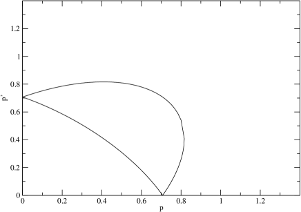
Figure 14: Logarithmically divergent moon-shape region of the matrix elements $Z(p^{\prime},p,E)$ of Eq.(85) of the Amado Model. $p$, $p^{\prime}$ and $E$ are in unit of $\hbar=2m=1$ with $E=1$.

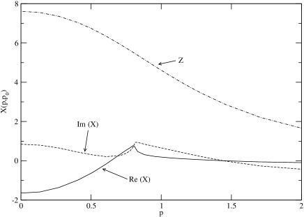
Figure 15: Half-off-shell amplitude $X(p,p_{0},E)$ of Eq.(85) of the Amado Model. $p$ and $p_{0}$ are in unit of $\hbar=2m=1$ with $E=1$. The dot-dashed curves are from deriveing term $Z(p,p_{0},E)$ of Eq.(85).

The choice of interpolation functions $S_{i}(p)$ depends on the property of the function to be interpolated. For example, the Lagrange interpolation polynomials are employed in Ref.r1 with some care near the breakup threshold. In the case of polynomial interpolation, however, some changes in a small region may give rise to global effects. Therefore it is better to use the spline interpolation which depends locally on the grids points, i.e., the function $S_{i}(p)$ dominates around the grid point $p_{i}$. Moreover, the spline interpolation is known to be less oscillating compared to the polynomial interpolation.

Spline functions are defined in terms of piecewise polynomials which are connected smoothly over the whole region. Since cubic splines are mostly employed, we will explain it in some detail. There are several kinds of spline functions depending on the condition of continuity. Among them, natural splines and Hermitean splines are very useful. Their characteristic properties are:

(1) natural splines: first and second derivatives are continuous at the grid points. It is a global spline in the sense that the function $S_{i}(p)$ depends on the whole grid points. It is known that the natural spline interpolation has a minimum curvature property.

(2) Hermitean splines: Only first derivatives are continuous at the grid points. It is a local spline in the sense that the function $S_{i}(p)\ (p_{i}\leq p\leq p_{i+1})$ depends on 4 grid points $\{p_{i-1},\ p_{i},\ p_{i+1},\ p_{i+2}\}$.

Since the practical ways of calculating the spline functions $S_{i}(p)$ are well described in Ref.r2 for natural splines and in Ref.r3 for Hermitean splines, we will not repeat them here.

The choice of spline functions certainly depends on the behavior of the solution $X(p,p_{0})$. As is well-known, there appears a square-root singularity at the breakup threshold r1 . More precisely, the amplitude $X(p,p_{0},E)$ goes like $(p_{B}-p)^{\ell+1/2}$ ( $\ell$ is an angular momentum of the 2-body bound state) below the breakup threshold $p_{B}$. Therefore, in the case of $\ell=0$, the derivative is not continuous at $p_{B}$ and there appears a sharp change of the amplitude. The straightforward application of the spline interpolation is not suitable since it requires the smooth continuation. One of the ways to take into account this singular threshold behavior is to divide the whole region $[0,\infty]$ into two regions $[0,p_{B}]\ [p_{B},\infty]$, and employ Hermitean spline interpolation in each region. It is also recommended that the grid points are suitably modified to account for the singularity near the breakup threshold, i.e., $p^{\prime}=\sqrt{p_{B}^{2}-p^{2}}\ (p\leq p_{B})$ and $p^{\prime}=\sqrt{p^{2}-p_{B}^{2}}\ (p\geq p_{B})$. In order to check the spline interpolation for the square-root singularity, it is a good exercise to fit the simple model function

$$f(x)=\left\{\begin{array}[]{ll}(1-x^{2})^{\ell+1/2}&\qquad 0\leq x\leq 1\\ (x^{2}-1)^{\ell+1/2}e^{-x}&\qquad 1\leq x<\infty\end{array}\right.$$ (91)

and to examine the accuracy of the interpolation. This exercise also will give some idea about the distribution of the grid points.

Now we will explain how the spline function method works in a calculation of Eq.(85) for the Amado model with the parameters $\hbar=2m=1,\ B=1.5,\ \beta=5,$ and the total energy $E=1$. As discussed above, the interaction $Z(p^{\prime},p,E)$ given in Eq.(86) is singular in the moon-shape region of Fig.14. To choose the grid points for solving Eq.(85) with the input Eqs.(86)-(87), we first identify some typical momenta: the on-shell momentum $p_{0}=\sqrt{4m(E+B)/3}$ of $bd$ elastic scattering, the tips of the moon-shape region on the coordinate axes $p_{end}=\sqrt{mE}$, the breakup threshold $p_{B}=\sqrt{4mE/3}$, and $p_{b}=\sqrt{mE/3}$ at which the moon-shape boundary has its maximum value from each coordinate axis. We then choose $p_{a}=0,\ p_{b}=\sqrt{mE/3}=0.408,\ p_{c}=p_{end}=\sqrt{mE}=0.707,\ p_{d}=p_{B}=\sqrt{4mE/3}=0.816,\ p_{f}=p_{0}=\sqrt{4m(E+B)/3}=1.291,\ p_{g}=p_{\rm max}=20$ and $p_{e}=(p_{d}+p_{f})/2=1.053$. These momenta are chosen to make 6 regions as $R_{a}=[p_{a},\ p_{b}],\ R_{b}=[p_{b},\ p_{c}],R_{c}=[p_{c},\ p_{d}],R_{d}=[p_{d},\ p_{e}],R_{e}=[p_{e},\ p_{f}],R_{f}=[p_{f},p_{g}]$. In addition to the grid points of those typical momenta, we prepare $\{2,2,4,3,3,9\}$ grid points in each region respectively, and thus 30 mesh points are used in solving the matrix equation Eq.(89) . They are distributed in equal space for $R_{a},\ R_{b}$ and $R_{e}$, while modified grid points $p_{i}^{\prime}$ are equally spaced near the breakup threshold for $R_{c}$ and $R_{d}$. In the region $R_{f}$, grid points are distributed as geometrical series with the ratio $r=1.5$ ;i.e., $p=1.291,\ 1.456,\ 1.704,\ 2.075,\ 2.632,\ 3.468,\ 4.722,\ 6.602,\ 9.423,\ 13.65,\ 20$ .

In order to evaluate the integral Eq.(90) accurately, we have employed 4-point Gauss-Legendre integration formula for each interval $[p_{n},\ p_{n+1}]$ which has no singularity. For the interval including the logarithmic singularity, we have changed the integration variable by explicitly taking account the location of the singularity as

$$\int_{p_{n}}^{p_{n+1}}dpF(p)=\int_{-t_{1}}^{t_{2}}dt3t^{2}F(p_{s}+t^{3})\ ,$$ (92)

where $p_{s}\ (p_{n}<p_{s}<p_{n+1})$ is the singular point. The variable is changed as $p=p_{s}+t^{3}$ and $t_{1}=(p_{s}-p_{n})^{1/3},\ t_{2}=(p_{n+1}-p_{s})^{1/3}$. This manipulation explicitly removes the logarithmic divergence from the integrand.

Thus, we have prepared two kinds of mesh points, i.e., one is the grid points $\{p_{i}\}$ at which the solution $X(p_{i},p_{0},E)$ is to be found by solving the matrix equation Eq.(89), and the other is to carry out the integration of Eq.(90) as precisely as required.

The calculated amplitude $X(p,p_{0},E)$ for zero total angular momentum are the solid curve (real part) and dashed curve (imaginary part) shown in Fig.15, which can be compared with the similar calculation of Ref. r5 . The amplitude $X(p,p_{0},E)$ is dimensionless and normalized as $X(p_{0},p_{0})=(\eta e^{2i\delta}-1)/(2i)$ at the on-shell point. One can see clearly the square-root singularity at the breakup threshold. We have also carried out the calculation with natural splines. Although natural splines are not suitable for the square-root singularity, it is practically possible to imitate the singularity by distributing many grid points around the breakup threshold. For example, the elastic amplitudes calculated by two different splines agree within the accuracy of 1%, since the on-shell point is away from the breakup threshold. In practice, both amplitudes coincides fairly well except for the small region around the breakup threshold. In Fig.15, we also show the contribution (dot-dashed curve) from the driving term $Z(p,p_{0},E)$ defined by Eq.(86). Its differences with the solid and dashed curves clearly show that the multiple scattering effects are very important.

The method described above can be readily extended to solve the coupled-channel equation Eq.(55). To be more specific, let us consider the case of $E=1.88$GeV. As discussed in the previous section, the partial-wave matrix elements of the driving terms $Z^{(E)}_{\pi\Delta,\pi\Delta}$ and $Z^{(E)}_{\rho N,\pi\Delta}$ of Eq.(55) diverge logarithmically in the moon-shape regions shown in Fig12. To choose the grid points for applying the spline function expansion method, we first select the following momenta

$$p_{0} = 0\ ,$$ (93)

$$p_{1} = \frac{m_{\pi}}{m_{N}+m_{\pi}}\ p_{6}\ ,$$ (94)

$$p_{2} = \frac{1}{2}\ p_{7}\ ,$$ (95)

$$p_{3} = \left[\frac{1}{4}(E-m_{N})^{2}-m_{\pi}^{2}\right]^{1/2}\ ,$$ (96)

$$p_{4} = \frac{m_{N}}{m_{N}+m_{\pi}}\ p_{6}\ ,$$ (97)

$$p_{5} = \left[\frac{1}{4}\left(E-m_{\pi}+\frac{m_{\pi}^{2}-m_{N}^{2}}{E-m_{\pi}}\right)^{2}-m_{\pi}^{2}\right]^{1/2}\ ,$$ (98)

$$p_{6} = \left[\frac{1}{4}\left(E+\frac{m_{\pi}^{2}-(m_{N}+m_{\pi})^{2}}{E}\right)^{2}-m_{\pi}^{2}\right]^{1/2}\ ,$$ (99)

$$p_{7} = \left[\frac{1}{4}\left(E+\frac{m_{N}^{2}-4m_{\pi}^{2}}{E}\right)^{2}-m_{N}^{2}\right]^{1/2}\ ,$$ (100)

$$p_{8} = \left[\frac{1}{4}\left(E+\frac{m_{N}^{2}-m_{\pi}^{2}}{E}\right)^{2}-m_{N}^{2}\right]^{1/2}\,.$$ (101)

The momentum $p_{8}$ is the on-shell momentum of the $\pi N$ state. $p_{6}(p_{7})$ corresponds to the momentum at which the invariant mass of the $\pi N$ ($\pi\pi)$ subsystem of the $\pi\pi N$ state is $m_{12}=m_{N}+m_{\pi}$ ($2m_{\pi}$). This momentum can be considered as the ”breakup” threshold of the unstable particle channels $\pi\Delta$ ($\rho N$ and $\sigma N$). Specifically, we take $\{p_{0},\ p_{1},\ p_{2},\ p_{3},\ p_{5},\ p_{6},\ p_{7},\ p_{8},\ p_{max}\}$ for $\pi$-spectator channel $(\pi N,\pi\Delta)$, and $\{p_{0},\ p_{1},\ p_{2},\ p_{4},\ p_{5},\ p_{6},\ p_{7},\ p_{8},\ p_{max}\}$ for $N$-spectator channel $(\rho N,\sigma N)$. For example, numerical values at $E=1.88$ GeV are : $p_{1}=80.29,\ p_{2}=334.8,\ p_{3}=448.7,\ p_{4}=539.1,\ p_{5}=605.8,\ p_{6}=619.4,\ p_{7}=669.7,\ p_{8}=696.3$ and $p_{max}=6000$. For 8 regions $R_{1}=[p_{0},\ p_{1}],\ R_{2}=[p_{1},\ p_{2}],\ldots,R_{8}=[p_{8},\ p_{max}]$, we prepare $\{3,\ 3,\ 3,\ 3,\ 3,\ 3,\ 3,\ 8\}$ grid points. The distribution of the mesh points and the integration over each region are the same as those for the Amado model.

It is a rather complex numerical task to get accurate solutions of Eq.(55). We check our numerical accuracy by reproducing the following optical theorem within $1\%$

$$\frac{4\pi}{k}Im[\hat{t}_{MB,MB}(\theta=0)]=\sum_{M^{\prime}B^{\prime}=\pi N,\eta N,\gamma N}\hat{\sigma}_{MB,M^{\prime}B^{\prime}}+\hat{\sigma}_{MB,\pi\pi N}$$ (102)

where $MB=\pi N,\eta N,\gamma N$ are stable particle channels, the cross sections $\hat{\sigma}_{a,b}$ are calculated from the non-resonant amplitudes $\hat{t}_{MB,M^{\prime}B^{\prime}}$ by solving Eq.(55). The two-pion production cross sections $\hat{\sigma}_{MB,\pi\pi N}$ are calculated from the amplitudes Eqs.(40)-(44) with resonant amplitude $t^{R}_{MB,M^{\prime}B^{\prime}}=0$.

VI Results

Our main interest in this paper is to use the numerical methods described in section V to examine the dynamical consequences of the one-particle-exchange interaction $Z^{(E)}_{\pi\Delta,\pi\Delta}$, $Z^{(E)}_{\rho N,\pi\Delta}$, and $Z^{(E)}_{\sigma N,\pi\Delta}$ (Fig.8). As illustrated in Fig.13 and discussed in section IV, the matrix elements of these interactions have logarithmically divergent structure due to the $\pi\pi N$ unitarity cuts which are not accounted for in all of the recent calculations of two-pion production. The parameters needed to evaluate the partial-wave matrix elements of $Z^{(E)}_{\pi\Delta,\pi\Delta}$, $Z^{(E)}_{\rho N,\pi\Delta}$, and $Z^{(E)}_{\sigma N,\pi\Delta}$ are fixed by the fitting the low-energy $\pi N$ and $\pi\pi$ scattering partial-wave amplitudes, as given in Appendices D and E. With the resonant amplitudes also fixed by using the information of PDG to evaluate Eqs.(66)-(72), our first task is to choose the parameters of starting Lagrangians, given in Appendix A, to evaluate the partial-wave matrix elements ${\it v}^{JT}_{L^{\prime}S^{\prime}M^{\prime}B^{\prime},LSMB}(k^{\prime},k)$ defined in Appendix C and ${\it v}^{JT}_{L^{\prime}S^{\prime}M^{\prime}B^{\prime},\lambda_{\gamma}\lambda_{N}}(k^{\prime},q)$ in Appendix F, with $MB,M^{\prime}B^{\prime}=\pi N,\eta N,\pi\Delta,\rho N,\sigma N$. Here we are guided by the previous works on meson-exchange models of $\pi N$ and $NN$ interactions, as discussed in Appendix A. We also need to regularize the resulting matrix elements of all of the non-resonant interactions given explicitly in Appendices C and F. This is done by multiplying each strong interaction vertex in the considered non-resonant mechanisms, illustrated in Figs.3-4, by a form factor $[\Lambda^{2}/(\Lambda^{2}+\vec{k}^{2})]^{2}$ with $\vec{k}$ being the momentum associated with the meson at the $MBB$ vertex or the meson being-exchanged. We adjust the cutoff parameters $\Lambda$ as well as some of the less well determined coupling constants to get a reasonable description of the Jlab data of invariant mass distributions of $\gamma p\rightarrow\pi^{+}\pi^{-}p$ reactions. With the parameters listed in Tables I-II of Appendix A, our results (solid curves) of the invariant mass distributions are compared with the data at $W=1.88$ GeV in Fig.16. While the improvements are clearly needed, the chosen parameters are sufficient for our present very limited purposes of investigating the effects due to $\pi\pi N$ cut. No attempt is made here to adjust the parameters to fit all of the available data of $\gamma p\rightarrow\pi^{+}\pi^{-}p,\pi^{0}\pi^{0}p,\pi^{+}\pi^{0}n$. This can be meaningfully pursued in a coupled-channel approach only when the data of $\pi N\rightarrow\pi N,\eta N,\pi\pi N$ and $\gamma N\rightarrow\pi N,\eta N$ are also considered. Here we focus on the effects due to the $\pi\pi N$ cut which are neglected in all recent two-pion production calculations..

To see the dynamical content of our calculations, we also show in Fig.16 the contributions from each of the unstable $\pi\Delta,\rho N,\sigma N$ channels. The $M_{\pi^{+}p}$ distribution (top panel) is clearly dominated by the process $\gamma p\rightarrow\pi\Delta\rightarrow\pi\pi N$ (dashed). The peak near $M_{\pi^{+}p}\sim 1.23$ GeV is dominated by the $\gamma p\rightarrow\pi^{-}(\Delta^{++}\rightarrow\pi^{+}p)$ process, while the shoulder in the $M_{\pi^{+}p}\sim 1.4-1.6$ region is due to the $\gamma p\rightarrow\pi^{+}(\Delta^{0}\rightarrow\pi^{-}p)$ process. The contributions from the $\rho N$ (dotted curve) and $\sigma N$ (dot-dashed curve) are sizable and can change the shape and magnitude of the cross sections through interference effects. The $M_{\pi^{+}\pi^{-}}$ distribution (middle panel) is dominated by $\gamma p\rightarrow p(\rho\rightarrow\pi^{+}\pi^{-})$ (dotted) and hence is peaked at $M_{\pi^{+}\pi^{-}}\sim 0.76$ GeV. However the contribution from $\pi\Delta$ channel (dashed) are clearly important in getting the good description of the data. The situation for $M_{\pi^{-}p}$ distribution (right) is similar to that for $M_{\pi^{+}p}$ distribution (bottom panel), except that the relative strength between two $\Delta$ peaks is changed.

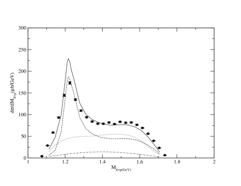
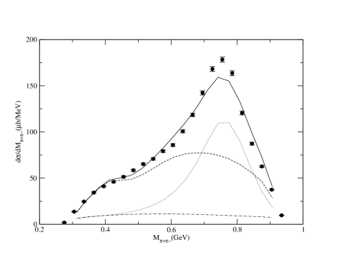
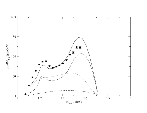
Figure 16: The differential cross sections of $\gamma p\rightarrow\pi^{+}\pi^{-}p$ reaction with respect to the invariant mass $M_{\pi^{+}p}$ (top), $M_{\pi^{+}\pi^{-}}$ (middle), and $M_{\pi^{-}p}$ (bottom) at W=1.880 GeV. The data are from Ref.mokeev-1 . The solid curves are from full calculations, The contributions from $\pi\Delta$ (dashed), $\rho N$ (dotted) and $\sigma N$ (dot-dashed) to the invariant mass distributions of $\gamma p\rightarrow\pi^{+}\pi^{-}p$ are also shown.

We now turn to investigating the effects due to the one-particle-exchange driving terms $Z_{\pi\Delta,\pi\Delta}^{(E)}(E)$,$Z_{\rho N,\pi\Delta}^{(E)}(E)$, and $Z_{\sigma N,\pi\Delta}^{(E)}(E)$ which contain the effects due to the $\pi\pi N$ unitarity cut, as discussed in section IV. Their singularity structure, illustrated in Fig.12, is similar to that shown in Fig.14 of the three-boson case. We thus expect that non-resonant partial-wave amplitudes associated with $\pi\Delta$, $\rho N$, and $\sigma N$ states have similar momentum-dependent structure of Fig.15. This is confirmed in our calculations. Some of our typical results are shown in Fig.17 for $t_{\pi\Delta,\pi N}$ and Fig.18 for the photo-production amplitudes $t_{\pi\Delta,\gamma N}$(upper panel) and $t_{\rho N,\gamma N}$(lower panel). The solid curves in these figures are from our full calculations, which show rapid varying structure. When the driving terms $Z_{\pi\Delta,\pi\Delta}^{(E)}(E)$, $Z_{\rho N,\pi\Delta}^{(E)}(E)$, and $Z_{\sigma N,\pi\Delta}^{(E)}(E)$ are turned off in solving Eq.(55), we obtain slow varying dashed curves. Here we note that the momentum variable $k$ in Figs.17-18 is related to the sub-energy $\sigma(k,E)=E-E_{s}(k)$ for the resonant particle ($\Delta$ or $\rho$) to decay in the presence of a spectator particle $s$ ($\pi$ or $N$) with energy $E_{s}(k)$. Thus the full curves in Figs.17-18 also reflect the rapid dependence on the sub-energy $\sigma(k,E)$. We emphasize that the rapid dependence of these amplitudes on the sub-energy $\sigma(k,E)$ is a necessary consequence of $\pi\pi N$ unitarity condition, as discussed by Aaron and Amadoaa-76 , and is similar to what can be seen in the $\pi NN$ studiesmatsuyama ; AM-1 ; AM-2 . Our results clearly indicate that the usual tree-diagram approximation should be used with cautions in interpreting the extracted $N^{*}$ parameters. The rapidly varying structure associated with an unstable particle channels must be taken into account in any phenomenological extraction of the partial-wave amplitudes. These were not taken into account in the early partial-wave analysesmanley-84 of the data of $\pi N\rightarrow\pi\pi N$.

If we further turn off the multiple scattering mechanisms in solving coupled-channel equation Eq.(55), we get the dot-dashed curves in Figs.17-18. The large differences between the dash-dotted curves and the solid curves indicate the difference between the dynamical coupled-channel approaches and the recent tree-diagram models.

Figure 17: The half-off-shell amplitudes $\hat{t}_{\pi\Delta,\pi N}(k,k_{0},E)$. The invariant mass of the outgoing $\Delta$ is 1.232 GeV and the total energy is E=1.880 GeV. The left (right) hand sides are the real (imaginary) parts of the amplitudes with $\pi N$ in $S_{11}$ (top) and $P_{31}$ (bottom). The partial-wave quantum numbers for $\pi\Delta$ state are indicated in each figure. The solid curves are from full coupled-channel calculations. The dashed curves are from setting $Z_{\pi\Delta,\pi\Delta}^{(E)}(E)=Z_{\rho N,\pi\Delta}^{(E)}(E)=Z_{\sigma N,\pi\Delta}^{(E)}(E)=0$. The dot-dashed curves are from further setting multiple scattering terms of Eq.(55) to zero; i.e. setting $\hat{t}^{JT}_{L^{\prime}S^{\prime}M^{\prime}B^{\prime},LSMB}(k^{\prime},k,E)={v}^{JT}_{L^{\prime}S^{\prime}M^{\prime}B^{\prime},LSMB}(k^{\prime},k,E)$. Note that the matrix elements of $v_{\pi\Delta,\pi N}$ are real in our phase convention (see Appendix A) and hence there is no dot-dashed curves in the right hand side.

Figure 18: The half-off-shell amplitudes $\hat{t}_{\pi\Delta,\gamma N}(k,q,E)$ (upper) and $\hat{t}_{\rho N,\gamma N}(k,q,E)$ (lower). The invariant mass of the outgoing $\Delta$ ($\rho$) is 1.232 GeV (0.76 GeV) and the total energy is E=1.880 GeV. The partial-wave quantum numbers for the final $\pi\Delta$ and $\rho N$ states are indicated in each figure. The solid curves are from full coupled-channel calculations. The dashed curves are from setting $Z_{\pi\Delta,\pi\Delta}^{(E)}(E)=Z_{\rho N,\pi\Delta}^{(E)}(E)=Z_{\sigma N,\pi\Delta}^{(E)}(E)=0$. The dot-dashed curves are from further setting multiple scattering terms of Eq.(65) to zero; i.e. setting $\hat{t}^{JT}_{LSMB,\lambda_{\gamma}\lambda_{N}m_{\tau_{N}}}(k^{\prime},k,E)={v}^{JT}_{LSMB,\lambda_{\gamma}\lambda_{N}m_{\tau_{N}}}(k^{\prime},k,E)$. Note that the matrix elements of $v_{\pi\Delta,\gamma N}$ ($v_{\rho N,\gamma N}$ ) are pure imaginary (real) in our phase convention (see Appendix A) and hence there is no dot-dashed curves in the right (left) sides of the upper (lower) parts.

We next examine the effects of the one-particle-exchange terms $Z_{\pi\Delta,\pi\Delta}^{(E)}(E)$, $Z_{\rho N,\pi\Delta}^{(E)}(E)$, and $Z_{\sigma N,\pi\Delta}^{(E)}(E)$ on the differential cross sections of $\gamma p\rightarrow\pi^{+}\pi^{-}p$. Here we set $\vec{p}$ as the outgoing $\pi^{+}$ momentum, $\vec{q}$ the relative momentum between $\pi^{-}$ and $p$. Two of our typical results of the dependence of the differential cross sections $d\sigma/(dM_{\pi^{-}p}d\Omega_{p}d\Omega_{q})$ on the azimuthal angle $\phi$ of $\vec{q}$ are shown in Fig.19 with the final $\pi^{+}\pi^{-}p$ kinematics fixed at $M_{\pi^{-}p}=1.23$GeV, $\cos\theta_{p}=0.183$, $\phi_{p}=-3.1$ rad., and $\cos\theta_{q}=0.80(left),0.183(right)$. Our full results are the solid curves. The dotted curves are obtained when $Z^{(E)}_{\pi\Delta,\pi\Delta}$, $Z_{\rho N,\pi\Delta}^{(E)}(E)$, and $Z_{\sigma N,\pi\Delta}^{(E)}(E)$ are turned off in solving the coupled-channel equation Eq.(55). Clearly, the effects due to these one-particle-exchange terms are very pronounced in changing both the shapes and magnitudes of the differential cross sections. Similar results are also seen in our calculations for other values of $\vec{p}$ of the outgoing $\pi^{+}$ and $\vec{q}$ of the relative momentum of the outgoing $\pi^{-}p$ system. The results shown in Fig.19 further indicate that the rapid varying structure of the amplitudes shown in Figs.17-18 must be accounted for in any analysis of two-pion production.

Figure 19: Differential cross sections of $\gamma p\rightarrow\pi^{+}\pi^{-}p$ at the $\gamma N$ invariant mass W=1.880 GeV. The outgoing $\pi^{+}$ momentum is $\vec{p}$ and the relative momentum between $\pi^{-}$ and $p$ is $\vec{q}$. $\phi$ is the azimuthal angle of $\vec{q}$. The results are for the invariant mass $M_{\pi^{-}p}=1.23$ GeV, $\cos\theta_{p}=0.183$, $\phi_{p}=-3.1$ rad. The left (right) panel is for $\cos\theta_{q}=0.80(0.183)$. The dashed curves are obtained when $Z^{(E)}_{MB,M^{\prime}B}$ term is turned off in solving Eq.(65).

In the recent studies of two-pion production, the data of invariant mass distributions $d\sigma/dM_{\pi N}$ and $d\sigma/dM_{\pi\pi}$ of $\gamma N\rightarrow\pi\pi N$ are most commonly used to extract $N^{*}$ parameters. Since these cross sections involve integrations over angles of outgoing particles, as seen in Eq.(74), the rapid varying structure of the partial-wave amplitudes due to $\pi\pi N$ cut is washed out. We thus see the smooth distributions $d\sigma/dM_{\pi N}$ and $d\sigma/dM_{\pi\pi}$, as shown in Figs.16. However the one-particle-exchange terms $Z_{\pi\Delta,\pi\Delta}^{(E)}(E)$, $Z_{\rho N,\pi\Delta}^{(E)}(E)$, and $Z_{\sigma N,\pi\Delta}^{(E)}(E)$ can change their magnitudes and shapes significantly. One example is shown in in Fig.20 for $\gamma p\rightarrow\pi^{0}\pi^{0}p$. We see that when these one-particle-exchange driving terms are turned off in solving coupled-channel equation Eq.(55), the predicted invariant mass distributions are reduced significantly. Such a large difference further indicate the importance of including the $\pi\pi N$ cut effects in calculating these particle-exchange terms for analyzing the two-pion production data.

Figure 20: The invariant mass distributions of $\gamma p\rightarrow\pi^{0}\pi^{0}p$ reaction at W=1.88 GeV. The dashed curves are obtained when $Z^{(E)}_{MB,M^{\prime}B}$ term is turned off in solving Eq.(65).

VII Summary and Future Developments

For analyzing the meson production data in the nucleon resonance ($N^{*}$) region, we have developed a dynamical coupled-channel reaction model. With the assumption that the basic degrees of freedom of the considered reactions are mesons ($M$) and baryons ($B$), our starting point is an energy-independent effective Hamiltonian which is derived from a set of Lagrangians by using a unitary transformation method. Within the constructed Hamiltonian, the $N^{*}$ excitations are defined by bare $N^{*}\rightarrow MB,\pi\pi N$ vertex interactions and the non-resonant meson-baryon interactions are defined by the tree-diagrams generated from the considered Lagrangians. We then apply the standard projection operator techniquesfeshbach to derive coupled-channel equations for calculating the amplitudes of meson-baryon reactions. The model satisfies the unitary conditions within the channel space spanned by the considered two-particle meson-baryon states and the three-particle $\pi\pi N$ state. In this paper, we present explicit formulations within a Fock-space spanned by the basis states $\gamma N$, $\pi N$, $\eta N$, $\pi\Delta$, $\rho N$, $\sigma N$, and $\pi\pi N$. However, the formulation can be straightforwardly extended to include other meson-baryon states such as Kaon-Hyperon (KY) and $\omega N$, and other two meson production channels such as $\eta\pi N$ and $K\bar{K}N$.

To facilitate the interpretations of the extracted $N^{*}$ parameters, we cast the reaction amplitudes into a form such that the meson-baryon scattering effects on $N^{*}$ excitations can be explicitly calculated. These effects, called the meson cloud effects, are due to the mechanisms that the incident meson interacts with the baryons through all possible non-resonant scattering before the $N^{*}$ is excited by the bare $N^{*}\rightarrow MB$ vertex interaction of the model Hamiltonian. The determination of the meson cloud effects from the meson production data could be useful for interpreting the extracted $N^{*}$ parameters in terms of hadron structure calculations. For example, it was found in Refs.sl-1 ; sl-2 that the meson cloud effects can account for the main differences between the extracted $\gamma N\rightarrow\Delta$ (1232) resonance transition form factors and the constituent quark model predictions. It will be interesting to explore how the meson cloud effects, as defined in our formulation, can be related to the $current$ Lattice QCD calculations.

In addition to giving a complete presentation of our theoretical framework, we also present in this paper a numerical method based on a spline-function expansion for solving the resulting coupled-channel equations which contain logarithmically divergent one-particle-exchange driving terms. These driving terms contain the effects due to the $\pi\pi N$ unitarity cuts which must be included accurately in calculating the two-pion production observables. We explain how this method can be applied in practice for a simple three-boson Amado model, and then for our realistic model with $\gamma N,\pi N,\pi\Delta,\rho N,\sigma N$, and $\pi\pi N$ channels.

An another important step in carrying out numerical calculations is to find an efficient way to calculate a large number of partial-wave matrix elements of the considered non-resonant meson-baryon interacting terms which are needed for solving the coupled-channel equations. Here we make use of the helicity representation of Jacob and Wick and also introduce a helicity-LSJ mixed-representation which is most convenient for calculating the electromagnetic matrix elements. While these are rather technical details, but are also presented explicitly in this paper for the completeness in explaining our numerics.

With the parameters of the model chosen appropriately to fit JLab’s two-pion photo-production data, we apply the developed numerical methods to show that the logarithmically divergent one-particle-exchange driving terms in the constructed coupled-channel equations generate rapid varying structure in the matrix elements of reaction amplitudes associated with unstable particle channels $\pi\Delta$, $\rho N$, and $\sigma N$. Our results confirm the analysis by Aaron and Amadoaa-76 . We further show that these one-particle-exchange terms have large effects in determining the two-pion production differential cross sections both in shapes and magnitudes. Our findings suggest that one needs to be cautious in interpreting the $N^{*}$ parameters extracted from the approaches which do not account for the effects due to the $\pi\pi N$ unitarity cuts.

The calculations presented in this paper are far from complete within our formulation, while they are sufficient for testing the accuracy of our numerical methods and illustrating the importance of $\pi\pi N$ unitarity cut. The $N^{*}$ parameters can be convincingly extracted and properly interpreted only when we apply our full formulation to analyze all available data of meson production reactions. Obviously this is a rather complex process. We now discuss how we will accomplish this rather ambitious research project in practice.

Our first task is to fit the $\pi N$ elastic scattering data to fix the parameters defining the strong interaction parts of the model Hamiltonian Eqs.(7)-(10). This must be done by extending the coupled-channel calculations described in section IV in two aspects, First, we must include the driving term $Z^{(I)}_{MB,M^{\prime}B^{\prime}}$ defined by Eq.(31). As discussed in section III, this term contains the $\pi\pi N$ cut effects originated from the $\pi NN$ vertex. Our second main task is to develop appropriate parameterizations of the bare $N^{*}\rightarrow MB$ form factors for calculating the resonant amplitudes rigorously according to Eqs.(15)-(19). Here we need to make use of the predictions from hadron structure calculations. For example, we at least can fix the relative phases between different $N^{*}\rightarrow MB$ transitions by using the naive SU(6) quark model with meson-quark coupling. Predictions from more sophisticated models, such as the ${}^{3}P_{0}$ model of Ref.capstick-roberts and the model based on Dyson-Schwinger Equationroberts , could provide useful information to our investigation. In fitting the $\pi N$ elastic scattering data, we should also fit the available $\pi N\rightarrow\eta N$ reaction data and use the optical theorem to make sure that the predicted $\pi N$ total cross sections are also in agreement with the data.

Once the $\pi N$ data are fitted by the above procedures, most of the strong interaction vertexes in the non-resonant electromagnetic interactions $v_{\gamma N,MB}$ and $v_{\gamma N\rightarrow\pi\pi N}$ of our model Hamiltonian have also been determined. We thus can focus on the determination of $\gamma N\rightarrow N^{*}$ form factors. From Eq.(19), one can use the operator relations Eqs.(B32)-(B33) of Appendix B to write the dressed $N^{*}\rightarrow\gamma N$ vertex of the resonant amplitude (Eq.(15)) as

$$\bar{\Gamma}_{N^{*}\rightarrow\gamma N}(E) = \Gamma_{N^{*}\rightarrow\gamma N}+\sum_{MB}\Gamma_{N^{*}\rightarrow MB}G_{MB}(E)t_{MB,\gamma N}(E)$$ (103)

$$\equiv \Gamma_{N^{*}\rightarrow\gamma N}+\sum_{MB}\bar{\Gamma}_{N^{*}\rightarrow MB}G_{MB}(E)v_{MB,\gamma N}.$$

Since $\bar{\Gamma}_{N^{*}\rightarrow MB}$ in the second line of the above equation has been determined in the fit to the $\pi N$ reaction data, the bare $N^{*}\rightarrow\gamma N$ vertex $\Gamma_{N^{*}\rightarrow\gamma N}$ is the main unknown and can be determined by fitting the data of photo-production and electro-production of $\pi,\eta$ and two pions. Of course some less well-determined parameters in the non-resonant interaction $v_{\gamma N,M^{\prime}B^{\prime}}$ should also be adjusted in the fits. In practice, one can extract bare $N^{*}\rightarrow\gamma N$ form factor at each $Q^{2}$. It of course will be more interesting if the parameterization of the bare form factor $\Gamma_{N^{*}\rightarrow\gamma N}$ can be guided by some theoretical calculations.

We now turn to discussing the extension of the model to include $KY$ and $\omega N$ channels which are also useful in probing the structure of $N^{*}$. In particular, we note that $\eta N,K\Lambda$, and $\omega N$ channels are of isospin $T=1/2$. The properties of $T=1/2$ $N^{*}$ states can therefore be more selectively extracted from analyzing the production data of these three channels. Thus, an extension of the formulation presented in this paper to include $KY$ and $\omega N$ channels is highly desirable and technically straightforward. However, it will increase the needed computation effort enormously. Nevertheless, we can make use of the results from fitting the $\pi N$, $\eta N$ and $\pi\pi N$ data to perform simplified coupled-channel analyses of the $KY$ and $\omega N$ production data. This can be done by following the approach of Ref.bruno .

Considering the $KY$ production, we assume that it can be described by a coupled-channel model including $\gamma N$, $KY$, $\pi N$, and a dummy channel $QQ$ which represent all of the neglected channels. If we further assume that $KY$ does not couple directly with the $QQ$ state (mainly because there is no information about how $KY$ couples with $\pi\pi N$ channels), one can cast the coupled-channel equation Eq.(24) into the following form

$$t_{\gamma N,KY}(E) = v_{\gamma N,KY}[1+G_{KY}(E)t_{KY,KY}(E)]+v_{\gamma N,\pi N}G_{\pi N}(E)t_{\pi N,KY}(E)$$ (104)

with

$$t_{KY,KY}(E) = v^{eff}_{KY,KY}(E)[1+G_{KY}(E)t_{KY,KY}(E)]\,,$$ (105)

$$t_{KY,\pi N}(E) = [1+t_{KY,KY}(E)G_{KY}(E)]v_{KY,\pi N}[1+G_{\pi N}(E)\hat{t}_{\pi N,\pi N}(E)]\,.$$ (106)

Here the effective $KY$ interaction is defined by

$$v^{eff}_{KY,KY}(E)=v_{KY,KY}+v_{KY\pi N}G_{\pi N}(E)[1+\hat{t}_{\pi N,\pi N}(E)G_{\pi N}(E)]v_{\pi N,KY}\,,$$ (107)

and $\hat{t}_{\pi N,\pi N}$ is from solving the coupled-channel equation Eq.(24) in the $\pi N\oplus QQ$ space.

If we assume that the dummy channel $QQ=\eta N\oplus\pi\Delta\oplus\rho N\oplus\sigma N$, the scattering amplitude $\hat{t}_{\pi N,\pi N}$ in the above equations is just the solution of Eq.(24) of the model determined in the fit to $\pi N$ data described above. We therefore can use this information to solve Eqs.(105)-(107) and determine the parameters associated with the non-resonant interaction $v_{KY,\pi N}$ and $v_{KY,KY}$ by fitting the available data of $\pi N\rightarrow KY$ reactions. This will then allow us to generate $t_{KY,KY}$ and $t_{\pi N,KY}$ to evaluate Eq.(104) and also fix the strong vertexes in the non-resonant $v_{\gamma N,KY}$. The $K\Lambda$ photo-production and electro-production data can then be used to extract the $\gamma N\rightarrow N^{*}$ form factors for $T=1/2$ $N^{*}$ states. The same procedure can be used to analyze the $\omega N$ production data.

To end this paper, we would like to emphasize here that the objective of performing dynamical coupled-channel analyses of meson production data is not only to extract the $N^{*}$ parameters, but also to provide information on reaction mechanisms for interpreting the extracted $N^{*}$ parameters in terms of the quark-gluon substructure of hadrons. In particular, we account for the dynamical consequences of the $\pi\pi N$ unitarity condition which is very difficult, if not impossible, to be treated rigorously in the existing approaches for calculating the hadron structure or the Lattice QCD calculations. An another important point to note is that our approach accounts for the off-shell scattering effects which describe the meson-baryon scattering wavefunctions in the short range region where we want to explore the structure of $N^{*}$. These essential quantum-mechanical effects are absorbed in the parameters of the approaches based on tree-diagram models or K-matrix models. Thus our dynamical approach perhaps has a better chance than these two approaches in revealing the quark-gluon substructure of baryons. Our progress in this direction will be publishedjlms elsewhere.

We would like to thank B. Julia-Diaz and K. Tsushima for their help in checking our calculations of the matrix elements of non-resonant interactions. This work is supported by the U.S. Department of Energy, Nuclear Physics Division, under Contract No. W-31-109-ENG-38 and the Japan Society for the Promotion of Science Grant-in-Aid for Scientific Research (C) 15540275.

Appendix A Lagrangian

In this appendix, we specify a set of Lagrangians for deriving the non-resonant interactions $v_{MB,M^{\prime}B^{\prime}}$ which is the input to the coupled-channel equations Eq.(24). Here we are guided by the previous works on meson-exchange models of $\pi N$ and $NN$ interactions. The coupling with pseudo-scalar mesons $\pi$ and $\eta$ are consistent with chiral symmetry. The vector meson couplings are less known and are mainly constructed phenomenologically. In the convention of Bjoken and Drellbj ), the Lagrangian with $\pi$, $\eta$, $N$, and $\Delta$ fields are

$$L_{\pi NN} = -\frac{f_{\pi NN}}{m_{\pi}}\bar{\psi}_{N}\gamma_{\mu}\gamma_{5}\vec{\tau}\psi_{N}\cdot\partial^{\mu}\vec{\phi_{\pi}}\,,$$ (108)

$$L_{\pi N\Delta} = -\frac{f_{\pi N\Delta}}{m_{\pi}}\bar{\psi}_{\Delta}^{\mu}\vec{T}\psi_{N}\cdot\partial_{\mu}\vec{\phi_{\pi}}\,,$$ (109)

$$L_{\pi\Delta\Delta} = \frac{f_{\Delta\Delta\pi}}{m_{\pi}}\bar{\psi}_{\Delta\mu}\gamma^{\nu}\gamma_{5}\vec{T}_{\Delta}\psi_{\Delta}^{\mu}\cdot\partial_{\nu}\vec{\phi}_{\pi}\,,$$ (110)

$$L_{\eta NN} = -\frac{f_{\eta NN}}{m_{\eta}}\bar{\psi}_{N}\gamma_{\mu}\gamma_{5}\psi_{N}\partial^{\mu}\phi_{\eta}\,.$$ (111)

The interactions involving $\rho$ meson are

$$L_{\rho NN} = g_{\rho NN}\bar{\psi}_{N}[\gamma_{\mu}-\frac{\kappa_{\rho}}{2m_{N}}\sigma_{\mu\nu}\partial^{\nu}]\vec{\rho^{\mu}}\cdot\frac{\vec{\tau}}{2}\psi_{N}\,,$$ (112)

$$L_{\rho N\Delta} = -i\frac{f_{\rho N\Delta}}{m_{\rho}}\bar{\psi}_{\Delta}^{\mu}\gamma^{\nu}\gamma_{5}\vec{T}\cdot[\partial_{\mu}\vec{\rho_{\nu}}-\partial_{\nu}\vec{\rho_{\mu}}]\psi_{N}+[h.c.]\,,$$ (113)

$$L_{\rho\Delta\Delta} = g_{\rho\Delta\Delta}\bar{\psi}_{\Delta\alpha}[\gamma^{\mu}-\frac{\kappa_{\Delta\Delta\rho}}{2m_{\Delta}}\sigma^{\mu\nu}\partial_{\nu}]\vec{\rho_{\mu}}\cdot\vec{T}_{\Delta}\psi_{\Delta}^{\alpha}\,,$$ (114)

$$L_{\rho\pi\pi} = g_{\rho\pi\pi}[\vec{\phi_{\pi}}\times\partial_{\mu}\vec{\phi_{\pi}}]\cdot\vec{\rho}^{\mu}\,,$$ (115)

$$L_{NN\rho\pi} = \frac{f_{\pi NN}}{m_{\pi}}g_{\rho NN}\bar{\psi}_{N}\gamma_{\mu}\gamma_{5}\vec{\tau}\psi_{N}\cdot\vec{\rho^{\mu}}\times\vec{\phi_{\pi}}\,,$$ (116)

$$L_{NN\rho\rho} = -\frac{\kappa_{\rho}g_{\rho NN}^{2}}{8m_{N}}\bar{\psi}_{N}\sigma^{\mu\nu}\vec{\tau}\psi_{N}\cdot\vec{\rho_{\mu}}\times\vec{\rho_{\nu}}\,.$$ (117)

Note that the contact terms Eqs.(116)-(117) are from applying $[\partial^{\mu}\rightarrow\partial^{\mu}-g_{\rho NN}\vec{\rho}^{\mu}\times]$ on $L_{\pi NN}$ Eq.(108) and $L_{\rho NN}$ Eq.(112).

The interactions involving $\omega$ meson are

$$L_{\omega NN} = g_{\omega NN}\bar{\psi}_{N}[\gamma_{\mu}-\frac{\kappa_{\omega}}{2m_{N}}\sigma_{\mu\nu}\partial^{\nu}]{\omega^{\mu}}\psi_{N}\,,$$ (118)

$$L_{\omega\pi\rho} = -\frac{g_{\omega\pi\rho}}{m_{\omega}}\epsilon_{\mu\alpha\lambda\nu}\partial^{\alpha}\vec{\rho^{\mu}}\partial^{\lambda}\vec{\phi_{\pi}}\omega^{\nu}\,.$$ (119)

We also consider interaction involving a scalar isoscalar $\sigma$ meson

$$L_{\sigma NN} = g_{\sigma NN}\bar{\psi}_{N}\psi_{N}\phi_{\sigma}$$ (120)

$$L_{\sigma\pi\pi} = -\frac{g_{\sigma\pi\pi}}{2m_{\pi}}\partial^{\mu}\vec{\phi}_{\pi}\partial_{\mu}\vec{\phi}_{\pi}\phi_{\sigma}\,.$$ (121)

$\frac{f_{\pi NN}^{2}}{4\pi}$	$f_{\pi N\Delta}$	$\kappa_{\rho}$	$g_{\omega NN}$	$\kappa_{\omega}$		$g_{\rho NN}g_{\rho\pi\pi}$
0.08	2.049	1.825	11.5	0		38.4329

Table 1: Coupling constants determined in Ref.sl-1 .

$g_{\rho\pi\pi}$	$g_{\sigma\pi\pi}$	$g_{\omega\pi\rho}$	$g_{\rho NN}$	$f_{\eta NN}$	$g_{\sigma NN}$	$f_{\pi\Delta\Delta}$	$f_{\rho N\Delta}$	$f_{\rho\Delta\Delta}$	$\kappa_{\rho\Delta\Delta}$
6.1994	1.77	11.2	6.1994	1.77	12.8	1.78	-6.08	-4.30	6.1

Table 2: Coupling constants used in the calculations in this paper.

To proceed, we need to know the coupling constants of the above Lagrangians. The parameters determined from fitting the $\pi N$ data within the SL modelsl-1 are given in Table I. The $\rho,\sigma\rightarrow\pi\pi$ coupling constants can be estimated from fitting $\pi\pi$ phase shifts in the isobar modeljohnstone , as described in Appendix C. The decay width of $\omega\rightarrow\pi\rho$ can be used to estimate the coupling constant $g_{\omega\pi\rho}$. The $\eta NN$ coupling constant $f_{\eta NN}$ has been estimated in recent studies of $\eta$ production from $\pi N$ and $\gamma N$ reactions. The $\sigma NN$ coupling can be estimated from the previous works on $NN$ scattering. These parameters are adjusted around the values from these estimates to fit the JLab data of $\gamma p\rightarrow\pi^{+}\pi^{-}p$ reactions, as described in section VII. They are listed in Table II.

We have very little information on the coupling constants $f_{\pi\Delta\Delta}$, $f_{N\Delta\rho}$ and $f_{\rho\Delta\Delta}$. We simply follow the previous works and use the simple SU(6) quark model to determine them from the empirical values of the coupling constants $f_{\pi NN}$ and $g_{\rho NN}$. To be more informative, we here also describe how this procedure is used in practice.

First step is take the static-baryon limit of the matrix elements $<B^{\prime}|L_{MBB^{\prime}}|BM(q)>$ to define the effective $MBB^{\prime}$ Hamiltonian operators in the spin-isospin space of baryons. They are

$$H_{\pi NN} = i\frac{f_{\pi NN}}{m_{\pi}}\vec{\sigma}\cdot\vec{q}\tau^{\alpha}\,,$$ (122)

$$H_{\pi N\Delta} = i\frac{f_{\pi N\Delta}}{m_{\pi}}\vec{S}\cdot\vec{q}T^{\alpha}\,,$$ (123)

$$H_{\pi\Delta\Delta} = i\frac{f_{\pi\Delta\Delta}}{m_{\pi}}\frac{2}{3}\vec{S}_{\Delta}\cdot\vec{q}T^{\alpha}_{\Delta}\,,$$ (124)

$$H_{\rho NN} = i\frac{g_{\rho NN}(1+\kappa_{\rho})}{4m_{N}}\vec{\sigma}\times\vec{q}\cdot\vec{\epsilon}(\rho)\tau^{\alpha}\,,$$ (125)

$$H_{\rho N\Delta} = -i\frac{f_{\rho N\Delta}}{m_{\rho}}\vec{S}\times\vec{q}\cdot\vec{\epsilon}(\rho)T^{\alpha}\,,$$ (126)

$$H_{\rho\Delta\Delta} = -ig_{\rho\Delta\Delta}\frac{1+\kappa_{\rho\Delta\Delta}}{2m_{\Delta}}\frac{2}{3}\vec{S}_{\Delta}\times\vec{q}\cdot\vec{\epsilon_{\rho}}T^{\alpha}_{\Delta}\,.$$ (127)

Here, $\alpha$ is the isospin component of the considered meson, $\vec{S}$ and $\vec{T}$ are the spin and isospin operators of the $N$-$\Delta$ transition, $\vec{S_{\Delta}}$ and $\vec{T_{\Delta}}$ are the spin and isospin operators of the $\Delta$. Along with the usual Pauli operators $\vec{\sigma}$ and $\vec{\tau}$, they are defined by the following reduced matrix elements

$$<N||\sigma||N> = <N||\tau||N>=\sqrt{6}\,,$$ (128)

$$<\Delta||S||N> = <\Delta||T||N>=2\,,$$ (129)

$$<\Delta||S_{\Delta}||\Delta> = <\Delta||T_{\Delta}||\Delta>=\sqrt{15}$$ (130)

with the convention that

$$<j_{f}m_{f}|O^{I}_{M}|j_{i}m_{i}>=\frac{1}{\sqrt{2j_{f}+1}}<j_{f}m_{f}|j_{i}Im_{i}M><j_{f}||O^{I}||j_{i}>\,.$$ (131)

We next consider a simple meson-quark interaction Hamiltonian

$$H_{\pi qq} = \frac{f_{\pi qq}}{m_{\pi}}\sum_{i=1,3}i\vec{\sigma}_{i}\cdot\vec{q}\tau_{i}\,,$$ (132)

$$H_{\rho qq} = \frac{f_{\rho qq}}{m_{\rho}}\sum_{i=1,3}i\vec{\sigma}_{i}\times\vec{q}\cdot\vec{\epsilon}_{\rho}\tau_{i}\,,$$ (133)

where $\sigma_{i},\tau_{i}$ are the spin and isospin operators of the constituent quarks. By using the 0s constituent quark wavefunctions $\psi_{N,m_{s_{N}}m_{\tau_{N}}}$ and $\psi_{\Delta,m_{s_{\Delta}}m_{\tau_{\Delta}}}$ for the nucleon and $\Delta$ and the relations Eq.(128)-(131), we have the following relations between the matrix elements in the spin-isospin space

$$<\psi_{N,m^{\prime}_{s_{N}}m^{\prime}_{\tau_{N}}}|\sum_{i=1,3}\vec{\sigma}_{i}\tau_{i}|\psi_{N,m_{s_{N}}m_{\tau_{N}}}> = \frac{5}{3}<m^{\prime}_{s_{N}}m^{\prime}_{\tau_{N}}|\vec{\sigma}\tau|m^{\prime}_{s_{N}}m^{\prime}_{\tau_{N}}>\,,$$ (134)

$$<\psi_{\Delta,m^{\prime}_{s_{\Delta}}m^{\prime}_{\tau_{\Delta}}}|\sum_{i=1,3}\vec{\sigma}_{i}\tau_{i}|<\psi_{N,m_{s_{N}}m_{\tau_{N}}}> = 2\sqrt{2}<m^{\prime}_{s_{\Delta}}m^{\prime}_{\tau_{\Delta}}|\vec{S}T|m^{\prime}_{s_{N}}m^{\prime}_{\tau_{N}}>\,,$$ (135)

$$<\psi_{\Delta,m^{\prime}_{s_{\Delta}}m^{\prime}_{\tau_{\Delta}}}|\sum_{i=1,3}\vec{\sigma}_{i}\tau_{i}|\psi_{\Delta,m_{s_{\Delta}}m_{\tau_{\Delta}}}> = \frac{4}{3}<m^{\prime}_{s_{\Delta}}m^{\prime}_{\tau_{\Delta}}|\vec{S}_{\Delta}T_{\Delta}|m_{s_{\Delta}}m_{\tau_{\Delta}}>\,.$$ (136)

Using the above formula and assume that the matrix elements of the hadron Hamiltonians Eqs.(122)-(127) are equal to the matrix elements of the quark-meson Hamiltonian Eqs.(132)-(133) within the SU(6) chiral constituent quark model

$$<\psi_{B,m^{\prime}_{s_{B}},m^{\prime}_{\tau_{B}}}|H_{Mqq}|\psi_{B,m_{s_{B}},m_{\tau_{B}}}>=<m^{\prime}_{s_{B}},m^{\prime}_{\tau_{B}}|H_{MBB^{\prime}}|m_{s_{B}},m_{\tau_{B}}>\,,$$ (137)

we then obtain

$$f_{\pi NN} = \frac{5}{3}f_{\pi qq}\,,$$ (138)

$$f_{\pi N\Delta} = 2\sqrt{2}f_{\pi qq}\,,$$ (139)

$$\frac{2}{3}f_{\pi\Delta\Delta} = \frac{4}{3}f_{\pi qq}\,,$$ (140)

$$f_{\rho NN} = \frac{5}{3}f_{\rho qq}\,,$$ (141)

$$f_{\rho N\Delta} = -2\sqrt{2}f_{\rho qq}\,,$$ (142)

$$\frac{2}{3}f_{\rho\Delta\Delta} =- \frac{4}{3}f_{\rho qq}\,,$$ (143)

where we defined

$$f_{\rho NN} = \frac{g_{\rho NN}(1+\kappa_{\rho})}{4m_{N}}m_{\rho}\,,$$ (144)

$$f_{\rho\Delta\Delta} = g_{\rho\Delta\Delta}\frac{1+\kappa_{\rho\Delta\Delta}}{2m_{\Delta}}m_{\rho}\,.$$ (145)

From the above relations we finally have

$$f_{\pi N\Delta} = \sqrt{\frac{72}{25}}f_{\pi NN}\,,$$ (146)

$$f_{\pi\Delta\Delta} = \frac{6}{5}f_{\pi NN}\,,$$ (147)

$$f_{\rho N\Delta} = -\sqrt{\frac{72}{25}}f_{\rho NN}\,,$$ (148)

$$f_{\rho\Delta\Delta} = -\frac{6}{5}f_{\rho NN}\,.$$ (149)

By using the vector meson dominance assumption and the recently determined $\Delta$ magnetic moment, we can set

$$\kappa_{\rho\Delta\Delta}=6.1\,.$$ (150)

With the values in Eq.(150) and values listed in Table I, we can use Eqs.(144)-(149) to get $f_{\pi\Delta\Delta}$, $f_{\rho N\Delta}$ and $f_{\rho\Delta\Delta}$. The resulting values are also listed in Table II.

The electromagnetic interactions are obtained from the usual non-interacting Lagrangian and the above interaction Lagrangian by using the minimum substitution $\partial_{\mu}\rightarrow\partial_{\mu}-ieA_{\mu}$. The resulting Lagrangian are given below :

$$L_{\gamma NN} = \bar{\psi}_{N}[\hat{e}_{N}\gamma^{\mu}-\frac{\hat{\kappa}_{N}}{2m_{N}}\sigma^{\mu\nu}\partial_{\nu}]\psi_{N}A_{\mu}\,,$$ (151)

$$L_{\gamma\pi\pi} = [\vec{\phi}_{\pi}\times\partial^{\mu}\vec{\phi}_{\pi}]_{3}A_{\mu}\,,$$ (152)

$$L_{\gamma N\pi N} = \frac{f_{\pi NN}}{m_{\pi}}[\bar{\psi}_{N}\gamma^{\mu}\gamma_{5}\vec{\tau}\psi_{N})\times\vec{\phi}_{\pi}]_{3}A_{\mu}\,,$$ (153)

$$L_{\gamma\rho\rho} = [(\partial^{\mu}\vec{\rho^{\nu}}-\partial^{\nu}\vec{\rho^{\mu}})\times\vec{\rho}_{\nu}]_{3}A_{\mu}\,,$$ (154)

$$L_{\gamma\rho\pi\pi} = -g_{\rho\pi\pi}[(\vec{\rho^{\mu}}\times\vec{\phi}_{\pi})\times\vec{\phi}_{\pi}]_{3}A_{\mu}\,,$$ (155)

$$L_{\gamma N\pi\Delta} = \frac{f_{\pi N\Delta}}{m_{\pi}}[(\bar{\psi}_{\Delta}^{\mu}\vec{T}\psi_{N})\times\vec{\phi}_{\pi}]_{3}A_{\mu}\,,$$ (156)

$$L_{\gamma N\rho N} = g_{\rho NN}[\frac{\kappa_{\rho}}{2m_{N}}(\bar{\psi}_{N}\frac{\vec{\tau}}{2}\sigma^{\nu\mu}\psi_{N})\times\vec{\rho_{\nu}}]_{3}A_{\mu}\,,$$ (157)

$$L_{\gamma N\Delta} = -i\bar{\psi}_{\Delta}^{\mu}\Gamma^{em,\Delta}_{\mu\nu}T_{3}\psi_{N}A^{\nu}+(h.c.)\,,$$ (158)

$$L_{\gamma\rho\pi} = \frac{g_{\rho\pi\gamma}}{m_{\pi}}\epsilon_{\alpha\beta\gamma\delta}\vec{\phi}_{\pi}\cdot(\partial^{\gamma}\vec{\rho^{\delta}})(\partial^{\alpha}A^{\beta})\,,$$ (159)

$$L_{\gamma\omega\pi} = \frac{g_{\omega\pi\gamma}}{m_{\pi}}\epsilon_{\alpha\beta\gamma\delta}(\partial^{\alpha}A^{\beta})\phi_{\pi}^{3}(\partial^{\gamma}\omega^{\delta})\,,$$ (160)

$$L_{\gamma\rho\eta} = \frac{g_{\rho\eta\gamma}}{m_{\rho}}\epsilon^{\mu\nu\alpha\beta}\partial_{\mu}\rho_{\nu}^{3}\partial_{\alpha}A_{\beta}\phi_{\eta}\,,$$ (161)

$$L_{\gamma\rho\sigma} = -\frac{g_{\rho\sigma\gamma}}{m_{\rho}}(\partial_{\mu}\rho_{\nu}^{3})(\partial^{\mu}A^{\nu}-\partial^{\nu}A^{\mu})\sigma\,,$$ (162)

$$L_{\gamma\Delta\Delta} = \bar{\psi}_{\Delta}^{\eta}(T^{3}_{\Delta}+\frac{1}{2})[-\gamma^{\mu}g_{\eta\nu}+(g^{\mu}_{\eta}\gamma^{\nu}+g^{\mu}_{\nu}\gamma^{\eta})+\frac{1}{3}\gamma_{\eta}\gamma^{\mu}\gamma_{\nu}]\psi_{\Delta}^{\nu}A_{\mu}\,.$$ (163)

For Eq. (151), we have defined

$$\hat{e} = \frac{F_{1S}+F_{1V}\tau^{3}}{2}\,,$$ (164)

$$\hat{\kappa} = \frac{F_{2S}+F_{2V}\tau^{3}}{2}\,,$$ (165)

where $F_{1S}(0)=F_{1V}(0)=1$, $F_{2S}(0)=\mu_{p}+\mu_{n}-1\sim-0.12$ and $F_{2V}(0)=\mu_{p}-\mu_{n}-1\sim 3.7$ The matrix element of $\gamma N\Delta$ vertex of Eq. (156) between an $N$ with momentum $p$ and a $\Delta$ with momentum $p_{\Delta}$ can be written explicitly as

$$<\Delta(p_{\Delta}^{\prime})|\Gamma^{em\Delta}_{\mu\nu}|N(p_{N})>= \frac{m_{\Delta}+m_{N}}{2m_{N}}\frac{1}{(m_{\Delta}+m_{N})^{2}-q^{2}}$$ (166)

$$\times[(G_{M}-G_{E})3\epsilon_{\mu\nu\alpha\beta}P^{\alpha}q^{\beta}$$

$$+G_{E}i\gamma_{5}\frac{12}{(m_{\Delta}-m_{N})^{2}-q^{2}}\epsilon_{\mu\lambda\alpha\beta}P^{\alpha}q^{\beta}\epsilon^{\lambda}_{\ \ \nu\alpha\delta}p_{\Delta}^{\gamma}q^{\delta}$$

$$+G_{C}i\gamma_{5}\frac{6}{(m_{\Delta}-m_{N})^{2}-q^{2}}q_{\mu}(q^{2}P_{\nu}-q\cdot Pq_{\nu})],$$

with $P=(p_{\Delta}^{\prime}+p_{N})/2$ and $p_{\Delta}^{\prime}=p_{N}+q$. Note that the index $\mu$ of $\Gamma^{em\Delta}_{\mu\nu}$ contracts with the $\Delta$ field and $\nu$ with the photon field. The coupling strength $G_{M}=1.85$, $G_{E}=0.025$, and $G_{C}=-0.238$ are taken from the SL modelsl-1 ; sl-2 .

Appendix B Derivation of Coupled-channel Equations

In this appendix, we give the derivation of coupled-channel equations from the model Hamiltonian $H_{eff}=H_{0}+V$ defined by Eqs.(5)-(10). We apply the standard projection operator techniquesfeshbach . The procedure is similar to that used in the derivation of $\pi NN$ equationsLM85 . We start with Eq.(12)

$$T(E)=V+V\frac{1}{E-H_{0}}T(E)\,.$$ (167)

The propagator in the above equation is understood to include $+i\epsilon$ for defining the boundary condition, but is omitted to simplify the presentation in this appendix. The interaction $V$, defined in Eqs.(7)-(10), can be more clearly written as

$$V=v_{22}+v_{33}+(\Gamma_{12}+u_{23}+\gamma_{13})+(\Gamma_{21}+u_{32}+\gamma_{31})\,,$$ (168)

where $v_{22}=v_{MB,M^{\prime}B^{\prime}}+v_{\pi\pi}$, $\Gamma_{12}=\Gamma_{N^{*}\rightarrow MB}+h_{M^{*}\rightarrow\pi\pi}$ with $M^{*}=\rho,\sigma$, $\gamma_{13}=\Gamma_{N^{*}\rightarrow\pi\pi N}$, $u_{23}=v_{MB,\pi\pi N}$, and $v_{33}=v_{\pi\pi N\pi\pi N}$. Here we restrict $MB=\gamma N,\pi N,\eta N,\pi\Delta,\rho N,\sigma N$. In Eq.(168), we have also introduced more transparent notations $\Gamma_{21}=\Gamma^{\dagger}_{12}$, $u_{23}=u^{\dagger}_{23}$, and $\gamma_{31}=\gamma^{\dagger}_{13}$.

We next introduce projection operators

$$P+Q=1$$ (169)

with

$$Q = |\pi\pi N><\pi\pi N|\,,$$ (170)

$$P = P_{1}+P_{2}+P_{2*}\,,$$ (171)

where

$$P_{1} = \sum_{N^{*}}|N^{*}><N^{*}|\,,$$ (172)

$$P_{2} = |\gamma N><\gamma N|+|\pi N><\pi N|+|\eta N><\eta N|\,,$$ (173)

$$P_{2*} = |\pi\Delta><\pi\Delta|+|\rho N><\rho N|+|\sigma N><\sigma N|\,.$$ (174)

We then obtain the equations for the projected operators $T_{PP}=PTP$ and $T_{QP}=QTP$

$$T_{PP} = \bar{V}_{PP}+\bar{V}_{PP}\frac{1}{E-H_{0}}{T}_{PP}\,,$$ (175)

$$T_{QP} = \frac{1}{1-V_{QQ}\frac{Q}{E-H_{0}-V_{QQ}}}V_{QP}[1+\frac{P}{E-H_{0}}T_{PP}]\,,$$ (176)

where

$$\bar{V}_{PP}=V_{PP}+V_{PQ}\frac{Q}{E-H_{0}-V_{QQ}}V_{QP}\,,$$ (177)

with

$$V_{PP} = PVP=v_{22}+\Gamma_{12}+\Gamma_{21}\,,$$ (178)

$$V_{QP} = QVP=u_{32}+\Gamma_{21}+\gamma_{31}\,,$$ (179)

$$V_{QQ} = QVQ=v_{22}+v_{33}\,.$$ (180)

Eq.(177) can be written explicitly as

$$\bar{V}_{PP}=P[(v_{22}+\Gamma_{12}+\Gamma_{21})+(u_{23}+\gamma_{13}+\Gamma_{12})G_{Q}(u_{32}+\gamma_{31}+\Gamma_{21})]P\,,$$ (181)

with

$$G_{Q}=\frac{Q}{E-H_{0}-Q(v_{22}+v_{33})Q}\,.$$ (182)

From the definitions Eqs.(172)-(174) for the projection operators, we have the following conditions

$$P_{2}\Gamma_{12}Q = Q\Gamma_{12}P_{2}=0\,,$$

$$P_{2}\gamma_{31}Q = P_{2*}\gamma_{31}Q=Q\gamma_{31}P_{2}=Q\gamma_{31}P_{2*}=0\,.$$ (183)

With the above ”doorway” conditions, we can decompose $\bar{V}_{PP}$ as

$$\bar{V}_{PP}=P[\Sigma+\bar{v}]P\,,$$ (184)

where

$$\Sigma = [\Gamma_{12}G_{Q}\Gamma_{21}]_{un-connected}\,.$$ (185)

Here ${un-connected}$ in Eq.(185) means that the pion emitted from one baryon is also absorbed by the same baryon. Obviously this is the self-energy of the unstable particles in the $\pi\Delta$, $\rho N$ and $\sigma N$ states of $P_{2*}$ space. We thus have

$$P\Sigma P=P_{2*}\Sigma P_{2^{*}}\,.$$ (186)

All other interactions within the P-space are in $\bar{v}$ of Eq.(184)

$$\bar{v} = V_{E}+\hat{\Gamma}_{12}+\hat{\Gamma}_{21}+\hat{\Sigma}$$ (187)

with

$$V_{E} = v_{22}+(u_{23}+\Gamma_{12})G_{Q}(u_{32}+\Gamma_{21})-\Sigma\,,$$ (188)

$$\hat{\Gamma}_{21} = \Gamma_{21}++\Delta\hat{\Gamma}_{21}\,,$$ (189)

$$\hat{\Gamma}_{12} = \Gamma_{12}++\Delta\hat{\Gamma}_{12}\,,$$ (190)

$$\hat{\Sigma} = \gamma_{13}G_{Q}\gamma_{31}\,,$$ (191)

where $\Delta\hat{\Gamma}_{21}$ and $\Delta\hat{\Gamma}_{12}$ contain interactions due to $N^{*}\leftrightarrow\pi\pi N$ transitions

$$\Delta\hat{\Gamma}_{21}=[u_{23}+\Gamma_{21}]G_{Q}\gamma_{31}\,,$$ (192)

$$\Delta\hat{\Gamma}_{12}=\gamma_{13}G_{Q}[u_{32}+\Gamma_{12}]\,.$$ (193)

To follow the derivations given below, we note that the well known operator relations

$$t = v+v\frac{1}{E-H_{0}}t$$ (194)

$$= v+t\frac{1}{E-H_{0}}v$$

lead to

$$t = [1-v\frac{1}{E-H_{0}}]^{-1}v$$ (195)

$$= v[1-\frac{1}{E-H_{0}}v]^{-1}\,.$$

Eqs.(194) and (195) then lead to

$$[1-v\frac{1}{E-H_{0}}]^{-1} = 1+t\frac{1}{E-H_{0}}\,,$$

$$[1-\frac{1}{E-H_{0}}v]^{-1} = 1+\frac{1}{E-H_{0}}t\,.$$ (196)

Eq.(194) also leads to

$$t=v+v\frac{1}{E-H_{0}-v}v\,.$$ (197)

Comparing Eqs.(194) and (197), we have

$$\frac{1}{E-H_{0}-v}v = \frac{1}{E-H_{0}}t\,,$$

$$v\frac{1}{E-H_{0}-v} = t\frac{1}{E-H_{0}}\,.$$ (198)

It can also easily be seen that

$$\frac{1}{E-H_{0}-v}=\frac{1}{E-H_{0}}+\frac{1}{E-H_{0}}t\frac{1}{E-H_{0}}\,.$$ (199)

In the following derivations, the above relations Eqs.(194) -(199) will be often used without mentioned them again.

By using Eqs.(194), (197) and (199), we can write $T_{PP}$ defined by Eq.(175) as

$$T_{PP} = P[(\Sigma+v)+(\Sigma+v)\frac{1}{E-H_{0}-\Sigma+v}(\Sigma+v)]P$$ (200)

$$= P[\Sigma+\Sigma\frac{P_{2*}}{E-H_{0}-\Sigma}\Sigma+(1+\Sigma\frac{P_{2*}}{E-H_{0}-\Sigma})T_{\bar{v}}(1+\frac{P_{2*}}{E-H_{0}-\Sigma}\Sigma)]P$$

with

$$T_{\bar{v}}=\bar{v}+\bar{v}\frac{P}{E-H_{0}-\Sigma}T_{\bar{v}}\,.$$ (201)

By using Eq.(B13) and relation (B32), we can write Eq.(176) as

$$T_{QP}=Q[(1+t_{Q}\frac{Q}{E-H_{0}})(u_{32}+\gamma_{31}+\Gamma_{21})[1+\frac{P}{E-H_{0}}T_{PP}]P\,,$$ (202)

where

$$t_{Q}=V_{QQ}+V_{QQ}\frac{Q}{E-H_{0}}t_{Q}$$ (203)

describes $\pi\pi N\rightarrow\pi\pi N$ scattering through $V_{QQ}=Q[v_{22}+v_{33}]Q=v_{\pi\pi}+v_{\pi N,\pi N}+v_{\pi\pi N,\pi\pi N}$ interactions.

We now derive equations for calculating the scattering amplitudes between two particle channels in $P^{\prime}_{2}=P_{2}+P_{2*}$ space. We first note that

$$P^{\prime}_{2}\bar{v}P^{\prime}_{2} = V_{E}\,,$$ (204)

$$P^{\prime}_{2}\bar{v}P_{1} = \hat{\Gamma}_{21}\,,$$ (205)

$$P_{1}\bar{v}P^{\prime}_{2} = \hat{\Gamma}_{12}\,,$$ (206)

$$P_{1}\bar{v}P_{1} = \hat{\Sigma}\,.$$ (207)

The above relations and Eq.(B35) lead to

$$P^{\prime}_{2}T_{\bar{v}}P^{\prime}_{2} = V_{E}+V_{E}\frac{P^{\prime}_{2}}{E-H_{0}-\Sigma}P^{\prime}_{2}T_{\bar{v}}P^{\prime}_{2}+\hat{\Gamma}_{21}\frac{P_{1}}{E-m^{0}_{N^{*}}}P_{1}T_{\bar{v}}P^{\prime}_{2}\,,$$ (208)

$$P_{1}T_{\bar{v}}P^{\prime}_{2} = \hat{\Gamma}_{12}+\hat{\Gamma}_{12}\frac{P^{\prime}_{2}}{E-H_{0}-\Sigma}P^{\prime}_{2}T_{\bar{v}}P^{\prime}_{2}+\hat{\Sigma}\frac{P_{1}}{E-m^{0}_{N^{*}}}P_{1}T_{\bar{v}}P^{\prime}_{2}\,.$$ (209)

Eq.(209) can be written as

$$P_{1}T_{\bar{v}}P^{\prime}_{2} = [1-\hat{\Sigma}\frac{1}{E-m^{0}_{N^{*}}}]^{-1}[\hat{\Gamma}_{12}+\hat{\Gamma}_{12}\frac{P^{\prime}_{2}}{E-H_{0}-\Sigma}P^{\prime}_{2}T_{\bar{v}}P^{\prime}_{2}]$$ (210)

$$= \frac{E-m^{0}_{N^{*}}}{E-m^{0}_{N^{*}}-\hat{\Sigma}}[\hat{\Gamma}_{12}+\hat{\Gamma}_{12}\frac{P^{\prime}_{2}}{E-H_{0}-\Sigma}P^{\prime}_{2}T_{\bar{v}}P^{\prime}_{2}]\,.$$

Substituting Eq.(210) into Eq.(208), we have

$$P^{\prime}_{2}T_{\bar{v}}P^{\prime}_{2}=X+X\frac{1}{E-H_{0}-\Sigma}P^{\prime}_{2}T_{\bar{v}}P^{\prime}_{2}\,,$$ (211)

where

$$X=V_{E}+\hat{\Gamma}_{21}\frac{1}{E-M^{0}_{N^{*}}-\hat{\Sigma}}\hat{\Gamma}_{12}\,.$$ (212)

Eq.(211) can be written as

$$P^{\prime}_{2}T_{\bar{v}}P^{\prime}_{2} = [1-V_{E}\frac{1}{E-H_{0}-\Sigma}]^{-1}[V_{E}$$ (213)

$$+[1-V_{E}\frac{1}{E-H_{0}-\Sigma}]^{-1}\hat{\Gamma}_{21}\frac{1}{E-M^{0}_{N^{*}}-\hat{\Sigma}}\hat{\Gamma}_{12}[1+\frac{1}{E-H_{0}-\Sigma}P^{\prime}_{2}T_{\bar{v}}P^{\prime}_{2}]$$

$$= t_{E}+[1+t_{E}\frac{1}{E-H_{0}-\Sigma}]\hat{\Gamma}_{21}\frac{1}{E-M^{0}_{N^{*}}-\hat{\Sigma}}\hat{\Gamma}_{12}[1+\frac{1}{E-H_{0}-\Sigma}P^{\prime}_{2}T_{\bar{v}}P^{\prime}_{2}]$$

$$= t_{E}+\bar{\Gamma}_{21}\frac{1}{E-M^{0}_{N^{*}}-\hat{\Sigma}}\hat{\Gamma}_{12}[1+\frac{1}{E-H_{0}-\Sigma}P^{\prime}_{2}T_{\bar{v}}P^{\prime}_{2}]$$

$$= t_{E}+\bar{\Gamma}_{21}\frac{1}{E-M^{0}_{N^{*}}-\hat{\Sigma}}\hat{\Gamma}_{12}[1+\frac{1}{E-H_{0}-\Sigma-X}X]$$

$$= t_{E}+\bar{\Gamma}_{21}\frac{1}{E-M^{0}_{N^{*}}-\hat{\Sigma}}\hat{\Gamma}_{12}\frac{1}{E-H_{0}-\Sigma-X}[E-H_{0}-\Sigma]\,,$$

where

$$t_{E} = V_{E}+V_{E}\frac{1}{E-H_{0}-\Sigma}t_{E}\,,$$ (214)

$$\bar{\Gamma}_{21} = [1+t_{E}\frac{1}{E-H_{0}-\Sigma}]\hat{\Gamma}_{21}\,.$$ (215)

We further note that

$$\frac{1}{E-H_{0}-\Sigma-X} = \frac{1}{E-H_{0}-\Sigma-V_{E}-\hat{\Gamma}_{12}\frac{1}{E-M^{0}_{N^{*}}-\hat{\Sigma}}\hat{\Gamma}_{21}}$$ (216)

$$= \frac{1}{E-H_{0}-\Sigma-V_{E}}+\frac{1}{E-H_{0}-\Sigma-V_{E}}t_{s}\frac{1}{E-H_{0}-\Sigma-V_{E}}$$

with

$$t_{s} = \hat{\Gamma}_{12}\frac{1}{E-M^{0}_{N^{*}}-\hat{\Sigma}}\hat{\Gamma}_{21}[1+\frac{1}{E-H_{0}-\Sigma-V_{E}}t_{s}]$$ (217)

$$= \hat{\Gamma}_{12}\frac{1}{E-M^{0}_{N^{*}}-\hat{\Sigma}-\bar{\Sigma}}\hat{\Gamma}_{21}\,,$$

where

$$\bar{\Sigma} = \hat{\Gamma}_{12}\frac{1}{E-H_{0}-\Sigma-V_{E}}\hat{\Gamma}_{21}$$ (218)

$$= \hat{\Gamma}_{12}\frac{1}{E-H_{0}-\Sigma}\bar{\Gamma}_{21}\,.$$

Here $\bar{\Gamma}_{21}$ has been defined in Eq.(215).

By using Eqs.(216) and (217), Eq.(213) can be written as

$$P^{\prime}_{2}T_{\bar{v}}P^{\prime}_{2} = t_{E}+\bar{\Gamma}_{21}\frac{1}{E-M^{0}_{N^{*}}-\hat{\Sigma}}[1+(\hat{\Gamma}_{21}\frac{1}{E-H_{0}-\Sigma-V_{E}}\hat{\Gamma}_{12})\frac{1}{E-M^{0}_{N^{*}}-\hat{\Sigma}-\bar{\Sigma}}]$$

$$\times\hat{\Gamma}_{12}\frac{1}{E-H_{0}-\Sigma-V_{E}}[E-H_{0}-\Sigma]$$

$$= t_{E}+\bar{\Gamma}_{21}\frac{1}{E-M^{0}_{N^{*}}-\hat{\Sigma}}[1+\bar{\Sigma}\frac{1}{E-M^{0}_{N^{*}}-\hat{\Sigma}-\bar{\Sigma}}]\hat{\Gamma}_{12}\frac{1}{E-H_{0}-\Sigma-V_{E}}[E-H_{0}-\Sigma]$$

$$= t_{E}+\bar{\Gamma}_{21}\frac{1}{E-M^{0}_{N^{*}}-\hat{\Sigma}-\bar{\Sigma}}\hat{\Gamma}_{12}\frac{1}{E-H_{0}-\Sigma-V_{E}}[E-H_{0}-\Sigma]$$

$$= t_{E}+\bar{\Gamma}_{21}\frac{1}{E-M^{0}_{N^{*}}-\hat{\Sigma}-\bar{\Sigma}}\hat{\Gamma}_{12}[1+\frac{1}{E-H_{0}-\Sigma-V_{E}}V_{E}]$$

$$= t_{E}+\bar{\Gamma}_{21}\frac{1}{E-M^{0}_{N^{*}}-\hat{\Sigma}-\bar{\Sigma}}\hat{\Gamma}_{12}[1+\frac{1}{E-H_{0}-\Sigma}t_{E}]\,.$$

The above then gives

$$P^{\prime}_{2}T_{\bar{v}}P^{\prime}_{2} = t_{E}+\bar{\Gamma}_{21}\frac{1}{E-M^{0}_{N^{*}}-\hat{\Sigma}-\bar{\Sigma}}\bar{\Gamma}_{12}\,,$$ (219)

where (also recalling Eq.(215))

$$\bar{\Gamma}_{12} = \hat{\Gamma}_{12}[1+\frac{1}{E-H_{0}-\Sigma}t_{E}]\,,$$ (220)

$$\bar{\Gamma}_{21} = [1+t_{E}\frac{1}{E-H_{0}-\Sigma}]\hat{\Gamma}_{21}\,.$$ (221)

We now turn to deriving equations for calculating two-pion production. For initial $\pi N$ or $\gamma N$ of $P_{2}$-space, Eq.(202) can be written explicitly as

$$T_{QP_{2}} = Q(1+t_{Q}\frac{Q}{E-H_{0}})[u_{32}+u_{32}\frac{P_{2}}{E-H_{0}}T_{PP}P_{2}$$ (222)

$$+(u_{32}+\Gamma_{21})P_{2*}\frac{P_{2*}}{E-H_{0}}T_{PP}P_{2}+\gamma_{31}\frac{P_{1}}{E-H_{0}}T_{PP}P_{2}]\,.$$

From definition Eq.(200), we have

$$P_{2}T_{PP}P_{2} = P_{2}T_{\bar{v}}P_{2}\,,$$ (223)

$$P_{1}T_{PP}P_{2} = P_{1}T_{\bar{v}}P_{2}\,,$$ (224)

$$P_{2*}T_{PP}P_{2} = P_{2*}(1+\Sigma\frac{1}{E-H_{0}-\Sigma}P_{2*}]T_{\bar{v}}P_{2}$$ (225)

$$= P_{2*}[E-H_{0}]\frac{1}{E-H_{0}-\Sigma}P_{2*}T_{\bar{v}}P_{2}\,.$$

By using the above relations and Eq.(219) and $P^{\prime}_{2}=P_{2}+P_{2*}$, the 3rd in the bracket of Eq.(222) can be written as

$$3rd = (u_{32}+\Gamma_{21})\frac{P_{2^{*}}}{E-H_{0}-\Sigma}[t_{E}+\bar{\Gamma}_{21}\frac{1}{E-M^{0}_{N^{*}}-\hat{\Sigma}-\bar{\Sigma}}\bar{\Gamma}_{12}]P_{2}\,.$$ (226)

By using Eq.(B45), the 4th term in the bracket of Eq.(222) becomes

$$4th = \gamma_{31}\frac{1}{E-M^{0}_{N^{*}}-\hat{\Sigma}}\hat{\Gamma}_{12}[1+\frac{1}{E-H_{0}-\Sigma}P^{\prime}_{2}T_{\bar{v}}P^{\prime}_{2}]$$ (227)

$$= \gamma_{31}\frac{1}{E-M^{0}_{N^{*}}-\hat{\Sigma}}\hat{\Gamma}_{12}[1+\frac{1}{E-H_{0}-\Sigma}(t_{E}+\bar{\Gamma}_{21}\frac{1}{E-M^{0}_{N^{*}}-\hat{\Sigma}-\bar{\Sigma}}\bar{\Gamma}_{12})]$$

$$= \gamma_{31}\frac{1}{E-M^{0}_{N^{*}}-\hat{\Sigma}}[\hat{\Gamma}_{12}(1+\frac{1}{E-H_{0}-\Sigma}t_{E})+(\hat{\Gamma}_{12}\frac{1}{E-H_{0}-\Sigma}\bar{\Gamma}_{21})\frac{1}{E-M^{0}_{N^{*}}-\hat{\Sigma}-\bar{\Sigma}}\bar{\Gamma}_{12}]$$

$$= \gamma_{31}\frac{1}{E-M^{0}_{N^{*}}-\hat{\Sigma}}[1+\bar{\Sigma}\frac{1}{E-M^{0}_{N^{*}}-\hat{\Sigma}-\bar{\Sigma}}]\bar{\Gamma}_{12}$$

$$= \gamma_{31}\frac{1}{E-M^{0}_{N^{*}}-\hat{\Sigma}-\bar{\Sigma}}\bar{\Gamma}_{12}\,.$$

We finally obtain

$$T_{QP_{2}} = Q\Omega^{(-)\dagger}_{\pi\pi N}[u_{23}+\{u_{32}\frac{P_{2}}{E-H_{0}}+(u_{32}+\Gamma_{21})\frac{P_{2*}}{E-H_{0}-\Sigma}\}\{t_{E}+\bar{\Gamma}_{21}\frac{1}{E-M^{0}_{N^{*}}-\hat{\Sigma}-\bar{\Sigma}}\bar{\Gamma}_{12}\}$$ (228)

$$+\gamma_{31}\frac{1}{E-M^{0}_{N^{*}}-\hat{\Sigma}-\bar{\Sigma}}\bar{\Gamma}_{12}]P_{2}\,,$$

where

$$\Omega^{(-)\dagger}_{\pi\pi N}=(1+t_{Q}\frac{Q}{E-H_{0}})\,.$$ (229)

Here $t_{Q}$ is defined by Eq.(203) and hence $\Omega^{(-)\dagger}_{\pi\pi N}$ is the $\pi\pi N$ scattering operator.

In the above rather detailed derivations, Eqs.(B53) and (B62) are what we need to investigate meson-baryon scattering and two-pion production. In practice, the interaction $\gamma_{31}=\Gamma_{N^{*}\rightarrow\pi\pi N}$ will be neglected in first calculations. If we set $\gamma_{31}=0$, we then find from Eqs.(B23)-(B27) that

$$\hat{\Gamma}_{21} \rightarrow \Gamma_{21}\,,$$ (230)

$$\hat{\Gamma}_{12} \rightarrow \Gamma_{12}\,,$$ (231)

$$\hat{\Sigma} \rightarrow 0\,.$$ (232)

Eqs.(B52), and (B54)-(B55) lead to

$$\bar{\Gamma}_{21} \rightarrow [1+t_{E}\frac{1}{E-H_{0}-\Sigma}]\Gamma_{21}\,,$$ (233)

$$\bar{\Gamma}_{12} \rightarrow \Gamma_{12}[1+\frac{1}{E-H_{0}-\Sigma}t_{E}]\,,$$ (234)

$$\bar{\Sigma} \rightarrow \Gamma_{12}\frac{1}{E-H_{0}-\Sigma}[1+t_{E}\frac{1}{E-H_{0}-\Sigma}]\Gamma_{21}$$ (235)

$$= \Gamma_{12}\frac{1}{E-H_{0}-\Sigma}\bar{\Gamma}_{21}\,.$$

Recalling Eq.(B7)-(B8) for the projection operators $P_{2}$ and $P_{2*}$, we can write

$$P^{\prime}_{2}=P_{2}+P_{2*}=\sum_{MB}|MB><MB|\,,$$ (236)

where $MB=\gamma N,\pi N,\eta N,\pi\Delta,\rho N,\sigma N$ include all meson-baryon states in the considered model space. Defining

$$T_{MB,M^{\prime}B^{\prime}}(E) = <MB|P^{\prime}_{2}T_{\bar{v}}P^{\prime}_{2}|M^{\prime}B^{\prime}>\,,$$ (237)

$$t_{MB,M^{\prime}B^{\prime}}(E) = <MB|t_{E}|M^{\prime}B^{\prime}>\,,$$ (238)

$$V_{MB,M^{\prime}B^{\prime}}(E) = <MB|V_{E}|M^{\prime}B^{\prime}>\,,$$

and

$$G_{MB}(E) = <MB|\frac{1}{E-H_{0}-\Sigma}|MB>\,,$$ (239)

using the simplifications Eqs.(B64)-(B69), Eq.(B22) for $V_{E}$, and Eq.(B48) for $t_{E}$, the matrix element of Eq.(B53) between two $MB$ states then become

$$T_{MB,M^{\prime}B^{\prime}}(E) = t_{MB,M^{\prime}B^{\prime}}(E)+t^{R}_{MB,M^{\prime}B^{\prime}}(E)\,,$$ (240)

where

$$t_{MB,M^{\prime}B^{\prime}}(E) = V_{MB,M^{\prime}B^{\prime}}(E)+\sum_{M^{\prime\prime}B^{\prime\prime}}V_{MB,M^{\prime\prime}B^{\prime\prime}}(E)G_{M^{\prime\prime}B^{\prime\prime}}(E)t_{M^{\prime\prime}B^{\prime\prime},M^{\prime}B^{\prime}}(E)\,,$$ (241)

with

$$V_{MB,M^{\prime}B^{\prime}}(E)=<MB|v_{22}+(u_{23}+\Gamma_{12})G_{Q}(u_{32}+\Gamma_{21})-\Sigma|M^{\prime}B^{\prime}>\,.$$ (242)

As defined in the beginning of this appendix, we have $v_{22}=v_{MB,M^{\prime}B^{\prime}}+v_{\pi\pi}$, $\Gamma_{12}=\Gamma_{N^{*}\rightarrow MB}+h_{M^{*}\rightarrow\pi\pi}$ with $M^{*}=\rho,\sigma$, $\Gamma_{21}=\Gamma^{\dagger}_{12}$ and $u_{23}=v_{MB,\pi\pi N}$, $u_{32}=u^{\dagger}_{23}$. Eq.(242) can be written explicitly as

$$V_{MB,M^{\prime}B^{\prime}}(E)=v_{MB,M^{\prime}B^{\prime}}+Z_{{M}{B},{M}^{\prime}{B}^{\prime}}(E)\,.$$ (243)

Here $Z_{{M}{B},{M}^{\prime}{B}^{\prime}}(E)$ contains the effects due to the coupling with $\pi\pi N$ states. It has the following form

$$Z_{{M}{B},{M}^{\prime}{B}^{\prime}}(E) = <{M}{B}\mid F\frac{P_{\pi\pi N}}{E-H_{0}-\hat{v}_{\pi\pi N}+i\epsilon}F^{\dagger}\mid{M}^{\prime}{B}^{\prime}>$$ (244)

$$-[\delta_{MB,M^{\prime}B^{\prime}}\Sigma_{MB}(E)]\,,$$

where

$$\Sigma_{MB}(E) = <MB|\Sigma|MB>\,,$$ (245)

$$F = g_{V}+v_{MB,\pi\pi N}$$ (246)

$$= [\Gamma_{\Delta\rightarrow\pi N}+h_{\rho\rightarrow\pi\pi}+h_{\sigma\rightarrow\pi\pi}]+v_{MB,\pi\pi N}\,,$$

$$\hat{v}_{\pi\pi N} = v_{\pi N,\pi N}+v_{\pi\pi}+v_{\pi\pi N,\pi\pi N}\,.$$ (247)

The resonant term in Eq.(240) is

$$t^{R}_{MB,M^{\prime}B^{\prime}}(E) = <MB|\bar{\Gamma}_{21}\frac{1}{E-H_{0}-\bar{\Sigma}}\bar{\Gamma}_{12}|MB>$$ (248)

$$= \sum_{N^{*}_{i},N^{*}_{j}}\bar{\Gamma}_{MB\rightarrow N^{*}_{i}}<N^{*}_{i}|\frac{1}{E-H_{0}-\bar{\Sigma}}|N^{*}_{j}>\bar{\Gamma}_{N^{*}_{j}\rightarrow M^{\prime}B^{\prime}}\,.$$

Note that $\Sigma$ in Eqs.(B73) and (B79) is defined by Eq.(B19). If we neglect the non-resonant interactions in $\pi\pi N$ $Q$-space, we then have

$$\Sigma \rightarrow [\Gamma_{12}\frac{Q}{E-H_{0}}\Gamma_{21}]_{un-connected}\,.$$ (249)

Since $\Gamma_{12}$ does not have a $N\rightarrow\pi N$, we obviously have $<\pi N|\Sigma|\pi N>=0$ and hence

$$G_{\pi N}(E) = \frac{1}{E-K_{\pi}(k)-K_{N}(p)+i\epsilon}\,,$$ (250)

$$G_{\pi\Delta}(E) = \frac{1}{E-K_{\pi}(k)-K_{\Delta}(p)-\Sigma_{\pi\Delta}(E-K_{\pi}(k))}\,,$$ (251)

$$G_{\rho N}(E) = \frac{1}{E-K_{\rho}(k)-K_{N}(p)-\Sigma_{\rho N}(E-K_{N}(p))}\,,$$ (252)

$$G_{\sigma N}(E) = \frac{1}{E-K_{\sigma}-K_{N}(p)-\Sigma_{\sigma N}(E-K_{N}(p))}\,,$$ (253)

where

$$\Sigma_{\pi\Delta}(\omega) = <\pi\Delta|\Gamma_{\Delta\rightarrow\pi N}\frac{1}{\omega-K_{\pi}(k)-K_{N}(p)+i\epsilon}\Gamma_{\pi N\rightarrow\Delta}|\pi\Delta>\,,$$ (254)

$$\Sigma_{\rho N}(\omega) = <\rho N|\Gamma_{\rho\rightarrow\pi\pi}\frac{1}{\omega-E_{\pi}(k_{1})-E_{\pi}(k_{2})+i\epsilon}\Gamma_{\pi\pi\rightarrow\rho}|\rho N>\,,$$ (255)

$$\Sigma_{\sigma N}(\omega) = <\sigma N|\Gamma_{\sigma\rightarrow\pi\pi}\frac{1}{\omega-E_{\pi}(k_{1})-E_{\pi}(k_{2})+i\epsilon}\Gamma_{\pi\pi\rightarrow\sigma}|\sigma N>\,.$$ (256)

In the above equations, $K_{\alpha}(p)=\sqrt{m_{\alpha}^{2}+\vec{p}^{2}}$ is the free energy operator defined by momentum operator $\vec{p}$.

When $N^{*}\rightarrow\pi\pi N$ is neglected, the two-pion production operator $T_{QP}$ defined in Eq.(B62) also becomes simpler, since its last term in the right-hand side does not contribute. By using Eqs.(B66), (B72) and (B77), the matrix element of Eq.(B62) $T_{\pi\pi N,MB}(E)=<\pi\pi N|T_{QP_{2}}|MB>$ can be written as

$$T_{\pi\pi N,MB}(E) = <\psi^{(-)}_{\pi\pi N}|u_{32}|MB>$$ (257)

$$+\sum_{M^{\prime}B^{\prime}}[<\psi^{(-)}_{\pi\pi N}u_{32}\frac{P^{\prime}_{2}}{E-H_{0}-\Sigma}|M^{\prime}B^{\prime}>T_{M^{\prime}B^{\prime},MB}$$

$$+<\psi^{(-)}_{\pi\pi N}|\Gamma_{21}\frac{P_{2*}}{E-H_{0}-\Sigma}|M^{\prime}B^{\prime}>T_{M^{\prime}B^{\prime},MB}]\,.$$

Recalling that $u_{32}=v_{\pi\pi N,MB}$, $\Gamma_{21}=\Gamma_{\pi N\rightarrow\Delta}+\Gamma_{\pi\pi\rightarrow\rho}+\Gamma_{\pi\pi\rightarrow\sigma}$, we can write Eq.(257) explicitly as

$$T_{\pi\pi N,MB}(E)=T^{dir}_{\pi\pi N,MB}(E)+T^{\pi\Delta}_{\pi\pi N,MB}(E)+T^{\rho N}_{\pi\pi N,MB}(E)+T^{\sigma N}_{\pi\pi N,MB}(E)$$ (258)

with

$$T^{dir}_{\pi\pi N,MB}(E) = <\psi^{(-)}_{\pi\pi N}(E)|\sum_{M^{\prime}B^{\prime}}v_{\pi\pi N,M^{\prime}B^{\prime}}|M^{\prime}B^{\prime}>[\delta_{M^{\prime}B^{\prime},MB}$$ (259)

$$+G_{M^{\prime}B^{\prime}}(E)T_{M^{\prime}B^{\prime},MB}(E)\,,$$

$$T^{\pi\Delta}_{\pi\pi N,MB}(E) = <\psi^{(-)}_{\pi\pi N}(E)|\Gamma_{\pi N\rightarrow\Delta}|\pi\Delta>G_{\pi\Delta}(E)T_{\pi\Delta,MB}(E)\,,$$ (260)

$$T^{\rho N}_{\pi\pi N,MB}(E) = <\psi^{(-)}_{\pi\pi N}(E)|h_{\pi\pi\rightarrow\rho}|\rho N>G_{\rho N}(E)T_{\rho N,MB}(E)\,,$$ (261)

$$T^{\sigma N}_{\pi\pi N,MB}(E) = <\psi^{(-)}_{\pi\pi N}(E)|h_{\pi\pi\rightarrow\sigma}|\sigma N>G_{\sigma N}(E)T_{\sigma N,MB}(E)\,.$$ (262)

Appendix C Matrix elements of meson-baryon potentials

To solve Eq.(55) for generating the non-resonant amplitudes, we need to first calculate the partial-wave matrix elements of meson-baryon non-resonant interactions $v_{MB,M^{\prime}B^{\prime}}$ generated from the Lagrangians specified in Appendix A, and the one-particle-exchange interaction $Z^{(E)}_{MB,M^{\prime}B^{\prime}}(E)$ defined by Eq.(30) and illustrated in Fig.8. In this appendix, we present formula for calculating the partial-wave matrix elements of $v_{MB,M^{\prime}B^{\prime}}$ with $MB,M^{\prime}B^{\prime}=\pi N,\eta N,\sigma N,\rho N,\pi\Delta$. The partial-wave matrix elements of $Z^{(E)}_{MB,M^{\prime}B^{\prime}}(E)$ will be given in Appendix D.

In general, each of the constructed $v_{MB,M^{\prime}B^{\prime}}$ consists of various combinations of tree-diagram mechanisms illustrated in Fig.3. They can be computed by the usual Feynman rules, except that the time components of the propagators of the intermediate states are specified by the unitarity transformation method, such that the resulting matrix elements are independent of the collision energy $E$ of Eq.(55) and free of any singularity on the real momentum axis. We will explain this feature of our model at the end of this appendix.

It is convenient to get the partial matrix elements by first evaluating the matrix elements of $v_{MB,M^{\prime}B^{\prime}}$ in helicity representation and then transforming them into the usual $|(LS)JT>$ representation with $J$, $T$, $L$, and $S$ denoting the total angular momentum, isospin, orbital angular momentum, and spin quantum numbers, respectively. For each meson-baryon ($MB$) state, we use $k$($p$) to denote the momentum of $M$($B$). In the center of mass frame, we thus have $\vec{p}=-\vec{k}$. Following the Jacob-Wick formulationjw , the partial-wave matrix elements of the non-resonant interaction $v_{MB,M^{\prime}B^{\prime}}$ can be written as

$${\it v}^{JT}_{L^{\prime}S^{\prime}M^{\prime}B^{\prime},LSMB}(k^{\prime},k,E) = \sum_{\lambda^{\prime}_{M}\lambda^{\prime}_{B}\lambda_{M}\lambda_{B}}[\frac{\sqrt{(2L+1)(2L^{\prime}+1)}}{2J+1}$$ (263)

$$\times<j^{\prime}_{M}j^{\prime}_{B}\lambda^{\prime}_{M}-\lambda^{\prime}_{B}\mid S^{\prime}S^{\prime}_{z}><L^{\prime}S^{\prime}0S^{\prime}_{z}\mid JS^{\prime}_{z}>$$

$$\times<j_{M}j_{B}\lambda_{M}-\lambda_{B}\mid SS_{z}><LS0S_{z}\mid JS_{z}>$$

$$\times<J,k^{\prime}\lambda^{\prime}_{M}-\lambda^{\prime}_{B}\mid v_{M^{\prime}B^{\prime},MB}\mid J,k\lambda_{M}-\lambda_{B}>]\,,$$

where $j_{M}$ and $j_{B}$ are the spins of the meson and baryon, respectively, and $\lambda_{M}$ and $\lambda_{B}$ are their helicities, and

$$<J,k^{\prime}\lambda^{\prime}_{M}-\lambda^{\prime}_{B}\mid v_{M^{\prime}B^{\prime},MB}\mid J,k\lambda_{M}-\lambda_{B}>$$

$$=2\pi\int_{-1}^{+1}d(\cos\theta)d^{J}_{\lambda^{\prime}_{M}-\lambda^{\prime}_{B},\lambda_{M}-\lambda_{B}}(\theta)$$

$$\times<(\vec{k}^{\prime},s^{\prime}_{M}\lambda^{\prime}_{M}),(-\vec{k}^{\prime},s^{\prime}_{B},-\lambda^{\prime}_{B})\mid v_{M^{\prime}B^{\prime},MB}\mid(\vec{k},s_{M}\lambda_{M}),(-\vec{k},s_{B},-\lambda_{B})>\,.$$

Here we have chosen the coordinates such that

$$\vec{k}^{\prime} = (k^{\prime}\sin\theta,0,k^{\prime}\cos\theta)\,,$$ (265)

$$\vec{k} = (0,0,k)\,,$$ (266)

and the helicity eigenstates are defined by

$$\hat{k}\cdot\vec{s}_{M}\mid M(\vec{k},s_{M}\lambda_{M})> = \lambda_{M}\mid M(\vec{k},s_{M}\lambda_{M})>\,,$$ (267)

$$[-\hat{k}\cdot\vec{s}_{B}]\mid B(-\vec{k},s_{B}\lambda_{B})> = \lambda_{B}\mid B(-\vec{k},s_{B}\lambda_{B})>\,.$$ (268)

Note the $-$ sign in Eq.(268).

Channels	$\pi N$	$\eta N$	$\sigma N$	$\rho N$	$\pi\Delta$
$\pi N$	1	2	4	7	11
$\eta N$		3	5	8	12
$\sigma N$			6	9	13
$\rho N$				10	14
$\pi\Delta$					15

Table 3: Labels for $v_{a,b}$ with $a,b$ = $\pi N$, $\eta N$, $\sigma N$, $\rho N$, and $\pi\Delta$

To evaluate the matrix elements in the right hand side of Eq.(C) with the normalization defined by Eq.(48), we define (suppress the helicity and isospin indices)

$$<k^{\prime}(j),p^{\prime}\mid v_{M^{\prime}B^{\prime},MB}\mid k(i),p> = \frac{1}{(2\pi)^{3}}\sqrt{\frac{m_{B}^{\prime}}{E_{B^{\prime}}(p^{\prime})}}\frac{1}{\sqrt{2E_{M^{\prime}}(k^{\prime})}}\sqrt{\frac{m_{B}}{E_{B}(p^{\prime})}}\frac{1}{\sqrt{2E_{M}(k)}}$$ (269)

$$\times\bar{u}_{B^{\prime}}(\vec{p^{\prime}})\bar{V}(n)u_{B}(\vec{p})$$

where $n$ defined the $MB\rightarrow M^{\prime}B^{\prime}$ transitions as specified in Table 3, and $i,j$ are the isospin indices of the mesons. We also have defined $q=k^{\prime}-k$ or $q=p-p^{\prime}$. The expressions of each term in Table 3 are given in the following subsections.

C.1 $\pi(k,i)+N(p)\rightarrow\pi(k^{\prime},j)+N(p^{\prime})$

$$\bar{V}(1)=\bar{V}^{1}_{a}+\bar{V}^{1}_{b}+\bar{V}^{1}_{c}+\bar{V}^{1}_{d}+\bar{V}^{1}_{e}$$ (270)

with

$$\bar{V}^{1}_{a} = [\frac{f_{\pi NN}}{m_{\pi}}]^{2}\not\!k^{\prime}\gamma_{5}\tau^{j}S_{N}(p+k)\not\!k\gamma_{5}\tau^{i}$$ (271)

$$\bar{V}^{1}_{b} = [\frac{f_{\pi NN}}{m_{\pi}}]^{2}\not\!k\gamma_{5}\tau^{i}S_{N}(p-k^{\prime})\not\!k^{\prime}\gamma_{5}\tau^{j}$$ (272)

$$\bar{V}^{1}_{c} = [\frac{f_{\pi N\Delta}}{m_{\pi}}]^{2}{k}_{\alpha}(T^{\dagger})^{i}S^{\alpha\beta}_{\Delta}(p-k^{\prime}){k}^{\prime}_{\beta}T^{j}$$ (273)

$$\bar{V}^{1}_{d} = ig_{\rho NN}g_{\rho\pi\pi}\frac{\tau^{\it l}}{2}\epsilon_{ji{\it l}}\frac{1}{q^{2}-m^{2}_{\rho}}$$ (274)

$$\times[(\not\!k+\not\!k^{\prime})+\frac{\kappa_{\rho}}{4m_{N}}\{(\not\!k+\not\!k^{\prime})\not\!q-\not\!q(\not\!k+\not\!k^{\prime})\}]$$

$$\bar{V}^{1}_{e} = -g_{\sigma NN}\frac{g_{\sigma\pi\pi}}{m_{\pi}}\delta_{i,j}\frac{k\cdot k^{\prime}}{q^{2}-m_{\sigma}^{2}}$$ (275)

C.2 $\pi(k,i)+N(p)\rightarrow\eta(k^{\prime})+N(p^{\prime})$

$$\bar{V}(2)=\bar{V}^{2}_{a}+\bar{V}^{2}_{b}$$ (276)

with

$$\bar{V}^{2}_{a} = \frac{f_{\pi NN}f_{\eta NN}}{m_{\pi}m_{\eta}}\not\!k^{\prime}\gamma_{5}S_{N}(p+k)\not\!k\gamma_{5}\tau^{i}$$ (277)

$$\bar{V}^{2}_{b} = \frac{f_{\pi NN}f_{\eta NN}}{m_{\pi}m_{\eta}}\not\!k\gamma_{5}\tau^{i}S_{N}(p-k^{\prime})\not\!k^{\prime}\gamma_{5}$$ (278)

C.3 $\eta(k)+N(p)\rightarrow\eta(k^{\prime})+N(p^{\prime})$

$$\bar{V}(3)=\bar{V}^{3}_{a}+\bar{V}^{3}_{b}$$ (279)

with

$$\bar{V}^{3}_{a} = [\frac{f_{\eta NN}}{m_{\eta}}]^{2}\not\!k^{\prime}\gamma_{5}S_{N}(p+k)\not\!k\gamma_{5}$$ (280)

$$\bar{V}^{3}_{b} = [\frac{f_{\eta NN}}{m_{\eta}}]^{2}\not\!k\gamma_{5}S_{N}(p-k^{\prime})\not\!k^{\prime}\gamma_{5}$$ (281)

C.4 $\pi(k,i)+N(p)\rightarrow\sigma(k^{\prime})+N(p^{\prime})$

$$\bar{V}(4)=\bar{V}^{4}_{a}+\bar{V}^{4}_{b}+\bar{V}^{4}_{c}$$ (282)

with

$$\bar{V}^{4}_{a} = ig_{\sigma NN}\frac{f_{\pi NN}}{m_{\pi}}S_{N}(p+k)\not\!k\gamma_{5}\tau^{i}$$ (283)

$$\bar{V}^{4}_{b} = ig_{\sigma NN}\frac{f_{\pi NN}}{m_{\pi}}\not\!k\gamma_{5}S_{N}(p-k^{\prime})\tau^{i}$$ (284)

$$\bar{V}^{4}_{c} = i\frac{f_{\pi NN}g_{\sigma\pi\pi}}{m_{\pi}^{2}}\not\!q\gamma_{5}\tau^{i}\frac{q\cdot k}{q^{2}-m^{2}_{\pi}}$$ (285)

C.5 $\eta(k)+N(p)\rightarrow\sigma(k^{\prime})+N(p^{\prime})$

$$\bar{V}(5)=\bar{V}^{5}_{a}+\bar{V}^{5}_{b}$$ (286)

with

$$\bar{V}^{5}_{a} = ig_{\sigma NN}\frac{f_{\eta NN}}{m_{\eta}}S_{N}(p+k)\not\!k\gamma_{5}$$ (287)

$$\bar{V}^{5}_{b} = ig_{\sigma NN}\frac{f_{\eta NN}}{m_{\eta}}\not\!k\gamma_{5}S_{N}(p-k^{\prime})$$ (288)

C.6 $\sigma(k)+N(p)\rightarrow\sigma(k^{\prime})+N(p^{\prime})$

$$\bar{V}(6)=\bar{V}^{6}_{a}+\bar{V}^{6}_{b}$$ (289)

with

$$\bar{V}^{6}_{a} = g_{\sigma NN}^{2}S_{N}(p+k)$$ (290)

$$\bar{V}^{6}_{b} = g_{\sigma NN}^{2}S_{N}(p-k^{\prime})$$ (291)

C.7 $\pi(k,i)+N(p)\rightarrow\rho(k^{\prime},j)+N(p^{\prime})$

$$\bar{V}(7)=\bar{V}^{7}_{a}+\bar{V}^{7}_{b}+\bar{V}^{7}_{c}+\bar{V}^{7}_{d}+\bar{V}^{7}_{e}$$ (292)

with

$$\bar{V}^{7}_{a} = i\frac{f_{\pi NN}}{m_{\pi}}g_{\rho NN}\Gamma_{\rho^{\prime}}S_{N}(p+k)\not\!k\gamma_{5}\tau^{i}$$ (293)

$$\bar{V}^{7}_{b} = i\frac{f_{\pi NN}}{m_{\pi}}g_{\rho NN}\not\!k\gamma_{5}\tau^{i}S_{N}(p-k^{\prime})\Gamma_{\rho^{\prime}}$$ (294)

$$\bar{V}^{7}_{c} = \frac{f_{\pi NN}}{m_{\pi}}g_{\rho\pi\pi}\epsilon_{ij{\it l}}\tau^{\it l}\frac{(q-k)\cdot\epsilon_{\rho^{\prime}}^{*}\not\!q\gamma_{5}}{q^{2}-m_{\pi}^{2}}$$ (295)

$$\bar{V}^{7}_{d} = -\frac{f_{\pi NN}}{m_{\pi}}g_{\rho NN}\not\!\epsilon_{\rho^{\prime}}^{*}\gamma_{5}\epsilon_{ji{\it l}}\tau^{\it l}$$ (296)

$$\bar{V}^{7}_{e} = \frac{g_{\omega NN}g_{\omega\pi\rho}}{m_{\omega}}\delta_{ij}\frac{\epsilon_{\alpha\beta\gamma\delta}\epsilon_{\rho^{\prime}}^{*\alpha}k^{\prime\beta}k^{\gamma}}{q^{2}-m^{2}_{\omega}}[\gamma^{\delta}+\frac{\kappa_{\omega}}{4m_{N}}(\gamma^{\delta}\not\!q-\not\!q\gamma^{\delta})]$$ (297)

where

$$\Gamma_{\rho^{\prime}} = \frac{\tau^{j}}{2}[\not\!\epsilon_{\rho^{\prime}}^{*}+\frac{\kappa_{\rho}}{4m_{N}}(\not\!\epsilon_{\rho^{\prime}}^{*}\not\!k^{\prime}-\not\!k^{\prime}\not\!\epsilon_{\rho^{\prime}}^{*})]$$ (298)

C.8 $\eta(k)+N(p)\rightarrow\rho(k^{\prime},j)+N(p^{\prime})$

$$\bar{V}(8)=\bar{V}^{8}_{a}+\bar{V}^{8}_{b}$$ (299)

with

$$\bar{V}^{8}_{a} = i\frac{f_{\eta NN}}{m_{\eta}}g_{\rho NN}\Gamma_{\rho^{\prime}}S_{N}(p+k)\not\!k\gamma_{5}$$ (300)

$$\bar{V}^{8}_{b} = i\frac{f_{\eta NN}}{m_{\eta}}g_{\rho NN}\not\!k\gamma_{5}S_{N}(p-k^{\prime})\Gamma_{\rho^{\prime}}$$ (301)

C.9 $\sigma(k)+N(p)\rightarrow\rho(k^{\prime},j)+N(p^{\prime})$

$$\bar{V}(9)=\bar{V}^{9}_{a}+\bar{V}^{9}_{b}$$ (302)

with

$$\bar{V}^{9}_{a} = g_{\rho NN}g_{\sigma NN}\Gamma_{\rho^{\prime}}S_{N}(p+k)$$ (303)

$$\bar{V}^{9}_{b} = g_{\rho NN}g_{\sigma NN}S_{N}(p-k^{\prime})\Gamma_{\rho^{\prime}}$$ (304)

C.10 $\rho(k,i)+N(p)\rightarrow\rho^{\prime}(k^{\prime},j)+N(p^{\prime})$

$$\bar{V}(10)=\bar{V}^{10}_{a}+\bar{V}^{10}_{b}+\bar{V}^{10}_{c}$$ (305)

with

$$\bar{V}^{10}_{a}+\bar{V}^{10}_{b} = g_{\rho NN}^{2}[\Gamma_{\rho^{\prime}}S_{N}(p+k)\Gamma_{\rho}+\Gamma_{\rho}S_{N}(p-k^{\prime})\Gamma_{\rho^{\prime}}]$$ (306)

where

$$\Gamma_{\rho} = \frac{\tau^{i}}{2}[\not\!\epsilon_{\rho}-\frac{\kappa_{\rho}}{4m_{N}}(\not\!\epsilon_{\rho}\not\!k-\not\!k\not\!\epsilon_{\rho})]$$ (307)

$$\bar{V}^{10}_{c} = i\frac{\kappa_{\rho}g^{2}_{\rho NN}}{8m_{N}}[\not\!\epsilon_{\rho}\not\!\epsilon_{\rho^{\prime}}^{*}-\not\!\epsilon_{\rho^{\prime}}^{*}\not\!\epsilon_{\rho}]\epsilon_{ij{\it l}}\tau^{\it l}$$ (308)

C.11 $\pi(k,i)+N(p)\rightarrow\pi^{\prime}(k^{\prime},j)+\Delta(p^{\prime})$

$$\bar{V}(11)=\bar{V}^{11}_{a}+\bar{V}^{11}_{b}+\bar{V}^{11}_{c}+\bar{V}^{11}_{d}+\bar{V}^{11}_{e}$$ (309)

with

$$\bar{V}^{11}_{a} = \frac{f_{\pi NN}f_{\pi N\Delta}}{m^{2}_{\pi}}T^{j}\epsilon_{\Delta}^{*}\cdot k^{\prime}S_{N}(p+k)\not\!k\gamma_{5}\tau^{i}$$ (310)

$$\bar{V}^{11}_{b} = \frac{f_{\pi NN}f_{\pi N\Delta}}{m^{2}_{\pi}}T^{i}\epsilon_{\Delta}^{*}\cdot kS_{N}(p-k^{\prime})\not\!k^{\prime}\gamma_{5}\tau^{j}$$ (311)

$$\bar{V}^{11}_{c} = i\frac{f_{\rho N\Delta}f_{\rho\pi\pi}}{m_{\rho}}\frac{\epsilon_{ji{\it l}}T^{\it l}}{q^{2}-m^{2}_{\rho}}[\epsilon_{\Delta}^{*}\cdot q(\not\!k+\not\!k^{\prime})\gamma_{5}-\epsilon_{\Delta}^{*}\cdot(k+k^{\prime})\not\!q\gamma_{5}]$$ (312)

$$\bar{V}^{11}_{d} = -\frac{f_{\pi\Delta\Delta}f_{\pi N\Delta}}{m^{2}_{\pi}}[\epsilon_{\Delta}^{*}]_{\mu}\not\!k^{\prime}\gamma_{5}T^{j}_{\Delta}S^{\mu\nu}_{\Delta}(p^{\prime}+k^{\prime})T^{i}k_{\nu}$$ (313)

$$\bar{V}^{11}_{e} = -\frac{f_{\pi\Delta\Delta}f_{\pi N\Delta}}{m^{2}_{\pi}}[\epsilon_{\Delta}^{*}]_{\mu}\not\!k\gamma_{5}T^{i}_{\Delta}S^{\mu\nu}_{\Delta}(p-k^{\prime})T^{j}k_{\nu}^{\prime}$$ (314)

C.12 $\eta(k)+N(p)\rightarrow\pi^{\prime}(k^{\prime},j)+\Delta(p^{\prime})$

$$\bar{V}(12)=\frac{f_{\eta NN}f_{\eta N\Delta}}{m_{\pi}m_{\eta}}T^{j}\epsilon_{\Delta}^{*}\cdot k^{\prime}S_{N}(p+k)\not\!k\gamma_{5}$$ (315)

C.13 $\sigma(k)+N(p)\rightarrow\pi^{\prime}(k^{\prime},j)+\Delta(p^{\prime})$

$$\bar{V}(13)=-ig_{\sigma NN}\frac{f_{\pi N\Delta}}{m_{\pi}}T^{j}\epsilon_{\Delta}^{*}\cdot k^{\prime}S_{N}(p+k)$$ (316)

C.14 $\rho(k,i)+N(p)\rightarrow\pi^{\prime}(k^{\prime},j)+\Delta(p^{\prime})$

$$\bar{V}(14)=\bar{V}^{14}_{a}+\bar{V}^{14}_{b}+\bar{V}^{14}_{c}+\bar{V}^{14}_{d}$$ (317)

with

$$\bar{V}^{14}_{a} = -i\frac{f_{\pi N\Delta}g_{\rho NN}}{m_{\pi}}T^{j}\epsilon_{\Delta}^{*}\cdot k^{\prime}S_{N}(p+k)\Gamma_{\rho}$$ (318)

$$\bar{V}^{14}_{b} = i\frac{f_{\pi N\Delta}g_{\rho NN}}{m_{\pi}}T^{i}[\epsilon_{\Delta}^{*}\cdot k\not\!\epsilon_{\rho}\gamma_{5}-\epsilon_{\Delta}^{*}\cdot\epsilon_{\rho}\not\!k\gamma_{5}]$$ (319)

$$\times S_{N}(p-k^{\prime})\not\!k^{\prime}\gamma_{5}\tau^{j}$$

$$\bar{V}^{14}_{c} = -i\frac{f_{\pi\Delta\Delta}f_{\rho N\Delta}}{m_{\pi}m_{\rho}}[\epsilon_{\Delta}^{*}]_{\alpha}\not\!k^{\prime}\gamma_{5}T^{j}_{\Delta}S^{\alpha\beta}_{\Delta}(p^{\prime}+k^{\prime})[k_{\beta}\not\!\epsilon_{\rho}\gamma_{5}-[\epsilon_{\rho}]_{\beta}\not\!k\gamma_{5}]T^{i}$$ (320)

$$\bar{V}^{14}_{d} = -i\frac{g_{\rho\Delta\Delta}f_{\pi N\Delta}}{m_{\pi}}[\epsilon_{\Delta}^{*}]_{\alpha}[\not\!\epsilon_{\rho}-\frac{\kappa_{\rho\Delta\Delta}}{4m_{\Delta}}(\not\!\epsilon_{\rho}\not\!k-\not\!k\not\!\epsilon_{\rho})]T_{\Delta}^{i}S^{\alpha\beta}_{\Delta}(p-k^{\prime})T^{j}k^{\prime}_{\beta}$$

C.15 $\pi(k,i)+\Delta(p)\rightarrow\pi^{\prime}(k^{\prime},j)+\Delta^{\prime}(p^{\prime})$

$$\bar{V}(15)=\bar{V}^{15}_{a}+\bar{V}^{15}_{b}+\bar{V}^{15}_{c}+\bar{V}^{14}_{d}$$ (322)

with

$$\bar{V}^{15}_{a} = [\frac{f_{\pi N\Delta}}{m_{\pi}}]^{2}\epsilon_{\Delta}^{\prime*}\cdot k^{\prime}T^{j}S_{N}(p+k)\epsilon_{\Delta}\cdot k(T^{i})^{\dagger}$$ (323)

$$\bar{V}^{15}_{b} = [\frac{f_{\pi\Delta\Delta}}{m_{\pi}}]^{2}\not\!k^{\prime}\gamma_{5}T^{j}_{\Delta}[\epsilon_{\Delta^{\prime*}}]_{\mu}S^{\mu\nu}_{\Delta}(p+k)[\epsilon_{\Delta}]_{\nu}\not\!k\gamma_{5}T^{i}_{\Delta}$$ (324)

$$\bar{V}^{15}_{c} = [\frac{f_{\pi\Delta\Delta}}{m_{\pi}}]^{2}\not\!k\gamma_{5}T^{i}_{\Delta}[\epsilon_{\Delta^{\prime*}}]_{\mu}S^{\mu\nu}_{\Delta}(p-k^{\prime})[\epsilon_{\Delta}]_{\nu}\not\!k^{\prime}\gamma_{5}T^{j}_{\Delta}$$ (325)

$$\bar{V}^{15}_{d} = ig_{\rho\Delta\Delta}g_{\rho\pi\pi}\frac{\epsilon_{ji{\it l}}T_{\Delta}^{\it l}}{q^{2}-m^{2}_{\rho}}\{(\not\!k+\not\!k^{\prime})+\frac{\kappa_{\rho\Delta\Delta}}{4m_{\Delta}}((\not\!k+\not\!k^{\prime})\not\!q-\not\!q(\not\!k+\not\!k^{\prime})\}\epsilon_{\Delta^{\prime*}}\cdot\epsilon_{\Delta}$$

The baryon propagators in Eqs.(C8)-(C64) are

$$S_{N}(p) = \frac{1}{\not\!p-m_{N}}\,,$$ (327)

$$S^{\mu\nu}_{\Delta}(p) = \frac{1}{3(\not\!p-m_{\Delta})}[2(-g^{\mu\nu}+\frac{p^{\mu}p^{\nu}}{m_{\Delta}^{2}})+\frac{\gamma^{\mu}\gamma^{\nu}-\gamma^{\nu}\gamma^{\mu}}{2}-\frac{p^{\mu}\gamma^{\nu}-p^{\nu}\gamma^{\mu}}{m_{\Delta}}]\,.$$ (328)

Eq.(328) is the simplest choice of many possible definitions of the $\Delta$ propagator. It is part of our phenomenology for this rather complex coupled-channel calculations.

Although the expressions Eqs.(C8)-(C64) look like the usual Feynman amplitudes, the unitary transformation method defines definite procedures in evaluating the time component of each propagator. For each propagator, the vertex interactions associated with its ends define either a ”virtual” process or a ”real” process. The real process is the process that can occur in free space such as $\Delta\rightarrow\pi N$. The virtual processes, such as the $\pi N\rightarrow N$, $\pi\Delta\rightarrow\Delta$, and $\pi\Delta\rightarrow N$ transitions, are not allowed by the energy-momentum conservation. The consequences of the unitary transformation is the following. When both vertex interactions are ’virtual’, the propagator is the average of the propagators calculated with two different momenta specified by the initial and final external momenta. For example, the propagator of $\bar{V}_{a}$ of Eq. (C9), which corresponds to $\pi(k)N(p)\rightarrow N\rightarrow\pi(k^{\prime})N(p^{\prime})$, should be evaluated by

$$S_{N}(p+k) \rightarrow \frac{1}{2}[S_{N}(p+k)+S_{N}(p^{\prime}+k^{\prime})]$$ (329)

$$=\frac{1}{2}[\frac{(E_{N}(p)+E_{\pi}(k))\gamma^{0}-\vec{\gamma}\cdot(\vec{p}+\vec{k})+m_{N}}{(E_{N}(p)+E_{\pi}(k))^{2}-(\vec{p}+\vec{k})^{2}-m_{N}^{2}}$$

$$+\frac{(E_{N}(p^{\prime})+E_{\pi}(k^{\prime}))\gamma^{0}-\vec{\gamma}\cdot(\vec{p^{\prime}}+\vec{k^{\prime}})+m_{N}}{(E_{N}(p^{\prime})+E_{\pi}(k^{\prime}))^{2}-(\vec{p^{\prime}}+\vec{k^{\prime}})^{2}-m_{N}^{2}}]\,.$$

One see clearly that the denominators of the above expression are independent of the collision energy $E$ of scattering equation Eq. (55) and finite in all real momentum region. This is the essence of the unitary transformation method in deriving the interactions from Lagrangians. When only one of the vertex interactions is ’real’, the propagator is evaluated by using the momenta associated with the ’virtual’ vertex. For example, the propagator of $V^{11}_{d}$ Eq.(C51), which corresponds to $\pi(k)N(p)\rightarrow\Delta\rightarrow\pi(k^{\prime})\Delta(p^{\prime})$ is $S^{\mu\nu}_{\Delta}(p^{\prime}+k^{\prime})$, not $S^{\mu\nu}_{\Delta}(p+k)$ or $[S^{\mu\nu}_{\Delta}(p^{\prime}+k^{\prime})+S^{\mu\nu}_{\Delta}(p+k)]/2$. The structure of its denominator is similar to that of Eq.(C67) and hence the resulting matrix elements are also independent of scattering energy $E$ and finite in all momentum region. The terms which have one ’real’ and one ’virtual’ vertex interactions are $\bar{V}^{4}_{c}$, $\bar{V}^{7}_{c}$, $\bar{V}^{11}_{b}$. Their corresponding intermediate momentum variables have been correctly specified. The average, such as that of Eq.(C67), must be used in all other terms of Eqs.(C8)-(C64). We note that there is no propagator in Eqs.(C8)-(C64) which is attached by two real processes such as $\pi N\rightarrow\Delta\rightarrow\pi N$. Such real processes are generated from $\Gamma_{V}$ of the Hamiltonian and included in the resonant term $t^{R}_{MB,M^{\prime}B^{\prime}}$ of Eq.(14).

Appendix D Matrix elements of vertex interactions

We need to have partial-wave matrix elements of vertex interactions $\Gamma_{\Delta\rightarrow\pi N}$, $h_{\rho\rightarrow\pi\pi}$, and $h_{\sigma\rightarrow\pi\pi}$ to evaluate the self-energy $\Sigma_{\alpha}$ with $\alpha=\pi\Delta,\rho N,\sigma N$ of Eqs.(59)-(61), and the one-particle-exchange interactions $Z^{(E)}_{\pi\Delta,\pi\Delta}$, $Z^{(E)}_{\rho N,\pi\Delta}$, and $Z^{(E)}_{\sigma N,\pi\Delta}$, illustrated in Fig.8

In consistent with the normalizations defined by Eqs.(48), we write the matrix element of the $\alpha(p_{\alpha})\rightarrow\beta(p_{\beta})+\gamma(p_{\gamma})$ vertex interaction $f_{\alpha,\beta\gamma}$ as

$$<\vec{p}_{\alpha};j_{\alpha}m_{j_{\alpha}}|f_{\alpha,\beta\gamma}|\vec{p^{\prime}}_{\alpha}\vec{q^{\prime}}_{\alpha};j_{\beta}m_{j_{\beta}}j_{\gamma}m_{j_{\gamma}}>=\delta(\vec{p}_{\alpha}-\vec{p^{\prime}}_{\alpha})$$

$$\times\sum_{allm^{\prime}s}<\bar{j}_{\alpha}m_{\bar{j}_{\alpha}}|l_{\alpha}s_{\alpha}m_{l_{\alpha}}m_{s_{\alpha}}><s_{\alpha}m_{s_{\alpha}}|j_{\beta}j_{\gamma}m_{j_{\beta}}m_{j_{\gamma}}>f_{n_{\alpha}}(q^{\prime}_{\alpha})Y_{l_{\alpha}m_{l_{\alpha}}}(\hat{q^{\prime}_{\alpha}})\,,$$ (330)

where $j_{\alpha}$ is the spin of the particle $\alpha$, $l_{\alpha}$ is the relative orbital angular momentum of the pair $(\beta,\gamma)$, $n_{\alpha}=[(l_{\alpha}(j_{\beta}j_{\gamma})s_{\alpha})]\bar{j}_{\alpha}]$ denotes collectively all quantum numbers specifying the interacting $(\beta,\gamma)$ pair, The momenta are related by relativistic kinematics

$$\vec{p^{\prime}}_{\alpha} = \vec{p^{\prime}}_{\beta}+\vec{p^{\prime}}_{\gamma}\,,$$ (331)

$$\vec{q^{\prime}}_{\alpha} = \vec{p^{\prime}}_{\beta}+\rho_{\alpha}(p^{\prime}_{\alpha},p^{\prime}_{\beta},x)\vec{p^{\prime}}_{\alpha}\,,$$ (332)

$$\vec{q^{\prime}}_{\beta} = -\vec{p^{\prime}}_{\alpha}-\rho_{\beta}(p^{\prime}_{\alpha},p^{\prime}_{\beta},x)\vec{p^{\prime}}_{\beta}\,,$$ (333)

where $x=\hat{p^{\prime}_{\alpha}}\cdot\hat{p^{\prime}_{\beta}}$, and

$$\rho_{\alpha}(p_{\alpha},p_{\beta},x) = \xi_{p_{\alpha}}^{-1/2}\left[\varepsilon_{p_{\beta}}+\vec{p}_{\alpha}\cdot\vec{p}_{\beta}(\varepsilon_{p_{\beta}}+\varepsilon_{\vec{p}_{\alpha}+\vec{p}_{\beta}}+\xi_{p_{\alpha}}^{1/2})^{-1}\right]\,,$$

$$\rho_{\beta}(p_{\alpha},p_{\beta},x) = \rho_{\alpha}(p_{\beta},p_{\alpha},x)\,,$$

$$\xi_{p_{\alpha}} = (\varepsilon_{p_{\beta}}+\varepsilon_{\vec{p}_{\alpha}+\vec{p}_{\beta}})^{2}-p_{\alpha}^{2}\,.$$

The form factor $g_{n_{\alpha}}(q^{\prime}_{\alpha})$ for $\rho\rightarrow\pi\pi$ and $\sigma\rightarrow\pi\pi$ are taken from Ref.johnstone and $\Delta\rightarrow\pi N$ are from SL model. They are related to phase shifts by

$$-[\sin\delta_{\alpha}(E)]e^{i\delta_{\alpha}}(E)=\frac{|f_{n_{\alpha}}(q_{0})|^{2}}{E-M^{0}_{\alpha}-\Sigma_{\alpha}(E)}$$ (334)

with

$$\Sigma_{\alpha}(E)=\int q^{2}dq\frac{|f_{n_{\alpha}}(q)|^{2}}{E-E_{\beta}(q)-E_{\gamma}(q)+i\epsilon}$$ (335)

Explicitly we have

$$f_{\Delta,\pi N}(q)=-\frac{f_{\pi N\Delta}}{m_{\pi}}\frac{1}{(2\pi)^{3/2}}\frac{1}{\sqrt{2E_{\pi}(q)}}\sqrt{\frac{E_{N}(q)+m_{N}}{2E_{N}(q)}}\sqrt{\frac{4\pi}{3}}q[\frac{q^{2}}{q^{2}+\Lambda_{\pi N\Delta}^{2}}]^{2}$$ (336)

with $f_{\pi N\Delta}=2.049$, $\Lambda_{\pi N\Delta}=3.29$ (fm)^-1, and $M^{0}_{\Delta}=1299.07$ MeV,

$$f_{\rho,\pi\pi}(q)=g_{\rho,\pi\pi}\frac{qr}{(1+(qr)^{2})^{2}}$$ (337)

with $g_{\rho,\pi\pi}=0.6684$ $m^{1/2}_{\pi}$, $r=0.428$ fm, and $M^{0}_{\rho}=811.7$ MeV,

$$g_{\sigma,\pi\pi}(q)=g_{\sigma,\pi\pi}\frac{1}{1+(qr)^{2}}$$ (338)

with $g_{\sigma,\pi\pi}=0.7550m^{1/2}_{\pi}$, $r=0.522$ fm, and $M^{0}_{\sigma}=896.8$ MeV.

Appendix E Matrix elements of $Z^{(E)}_{MB,M^{\prime}B^{\prime}}(E)$

With the matrix elements of the vertex interactions defined by Eqs.(D1)-(D4) of Appendix D, we can evaluate the partial-wave matrix elements of one-particle-exchange interaction $Z^{(E)}_{MB,M^{\prime}B^{\prime}}$. We use the cyclic notation $(\alpha,\beta,\gamma)$ to specify the particles involved in the vertex interaction $\alpha\rightarrow\beta+\gamma$. By using the angular momentum quantum numbers defined in Appendix D, we then define the basis state of a $MB$ system with a given total angular momentum $(JM)$ in the center of mass frame as

$$|N_{\alpha};p_{\alpha}JM>=|\{L_{\alpha}[(l_{\alpha}(j_{\beta}j_{\gamma})s_{\alpha})\bar{j}_{\alpha}j_{\alpha}]S_{\alpha}\}JM;p_{\alpha}>\,,$$ (339)

where we have introduced a concise notation $N_{\alpha}=[\{L_{\alpha}[(l_{\alpha}(j_{\beta}j_{\gamma})s_{\alpha})\bar{j}_{\alpha}j_{\alpha}]S_{\alpha}\}]$.

Following the standard procedures of Ref.thomas-review , one then obtained

$$Z^{J}_{N_{\beta},N_{\alpha}}(p_{\beta},p_{\alpha}) = <N_{\beta};p_{\beta}JM|G_{\pi\pi N}(E)|N_{\alpha};p_{\alpha}JM>$$ (340)

$$= \bar{\delta}_{\alpha,\beta}[p^{l_{\alpha}}_{\beta}]\,[p^{l_{\beta}}_{\alpha}]\sum_{L}\sum_{a=0}^{l_{\alpha}}\sum_{b=0}^{l_{\beta}}F^{L,b,a}_{n_{\beta},n_{\alpha}}(p_{\beta},p_{\alpha};E)A^{L,a,b}_{N_{\beta},N_{\alpha}}(p_{\alpha}/p_{\beta})^{a-b}\,,$$

where $\bar{\delta}_{\alpha,\beta}=1-{\delta}_{\alpha,\beta}$, and

$$A^{L,a,b}_{N_{\beta},N_{\alpha}} = (-1)^{R}\hat{l}_{\alpha}\hat{l}_{\beta}\hat{L}_{\alpha}\hat{L}_{\beta}\hat{S}_{\alpha}\hat{S}_{\beta}\hat{\bar{j}}_{\alpha}\hat{\bar{j}}_{\beta}\hat{s}_{\alpha}\hat{s}_{\beta}\hat{L}^{2}$$ (346)

$$\times \{\frac{(2l_{\alpha}+1)!(2l_{\beta}+1)!}{(2a)!(2b)!(2l_{\alpha}-2a)!(2l_{\beta}-2b)!}\}^{1/2}$$

$$\times \sum_{f\Lambda\Lambda^{\prime}}[\hat{f}\hat{\Lambda}\hat{\Lambda}^{\prime}]^{2}\left\{\begin{array}[]{ccc}S_{\alpha}&S_{\beta}&f\\ L_{\beta}&L_{\alpha}&J\end{array}\right\}\left\{\begin{array}[]{cccccccc}j_{\alpha}&&S_{\alpha}&&S_{\beta}&&j_{\beta}&\\ &\bar{j}_{\alpha}&&f&&\bar{j}_{\beta}&&j_{\gamma}\\ s_{\alpha}&&l_{\alpha}&&l_{\beta}&&s_{\beta}&\end{array}\right\}$$

$$\times \left\{\begin{array}[]{ccc}L_{\alpha}&L_{\beta}&f\\ \Lambda^{\prime}&\Lambda&L\end{array}\right\}\left\{\begin{array}[]{ccc}l_{\alpha}&l_{\beta}&f\\ a&l_{\beta}-b&\Lambda\\ l_{\alpha}-a&b&\Lambda^{\prime}\end{array}\right\}$$ (352)

$$\times \left(\begin{array}[]{ccc}\Lambda^{\prime}&L&L_{\beta}\\ 0&0&0\end{array}\right)\left(\begin{array}[]{ccc}\Lambda&L&L_{\alpha}\\ 0&0&0\end{array}\right)\left(\begin{array}[]{ccc}l_{\alpha}-a&b&\Lambda^{\prime}\\ 0&0&0\end{array}\right)\left(\begin{array}[]{ccc}a&l_{\beta}-b&\Lambda\\ 0&0&0\end{array}\right)$$ (361)

with $\hat{a}=\sqrt{2a+1}$ and

$$R=-J+L+L_{\alpha}+L_{\beta}+S_{\alpha}+S_{\beta}+\bar{j}_{\alpha}+\bar{j}_{\beta}+s_{\beta}+l_{\beta}-j_{\alpha}\,.$$ (362)

In the above equations, the usual 3-j, 6-j, 9-j, and 12-j symboles have been used to define the angular momentum coupling. The details can be found in Ref.thomas-review .

The three-body cut effects are in $F^{L}_{n_{\beta},n_{\alpha}}(p_{\beta},p_{\alpha};E)$ of Eq.(E2). They are calculated from the vertex functions $f_{n_{\alpha}}(q_{\alpha})$ by

$$F^{L,b,a}_{n_{\beta},n_{\alpha}}(p_{\beta},p_{\alpha};E)=\frac{1}{2}\int_{-1}^{+1}dx\frac{q^{-l_{\beta}}_{\beta}\rho_{\beta}^{b}(x)f^{\dagger}_{n_{\beta}}(q_{\beta})q^{-l_{\alpha}}_{\alpha}\rho_{\alpha}^{a}(x)f_{n_{\alpha}}(q_{\alpha})P_{L}(x)}{E-E_{\alpha^{\prime}}(-\vec{p}_{\alpha})-E_{\beta^{\prime}}(-\vec{p}_{\beta})-E_{\gamma}(\vec{p}_{\alpha}+\vec{p}_{\beta})+i\epsilon}\,,$$ (363)

where $x=\hat{p_{\alpha}}\cdot\hat{p_{\beta}}$ and the vertex function $f_{n_{\alpha}}$ defines $\alpha\rightarrow\beta^{\prime}+\gamma$ and $f_{n_{\beta}}$ defines $\gamma+\alpha^{\prime}\rightarrow\beta$. Namely, $\alpha^{\prime}$ and $\beta^{\prime}$ are the spectators of the decay of particle $\alpha$ and $\beta$ respectively. We obviously have $\alpha=\Delta$, $\alpha^{\prime}=\pi$, $\gamma=N$, $\beta=\Delta$ and $\beta^{\prime}=\pi$ for $Z^{(E)}_{\pi\Delta,\pi\Delta}(E)$, and $\alpha=\rho,\sigma$, $\alpha^{\prime}=N$, $\gamma=\pi$, $\beta=\Delta$ and $\beta^{\prime}=\pi$ for $Z^{(E)}_{\rho N,\pi\Delta}(E)$.

In the actual calculations, the integration path $-1\leq x\leq 1$ of eq.(E5) is deformed into the complex $x-$plane in order to avoid the singularity $x_{0}\ (-1\leq x_{0}\leq 1)$ where the denominator vanishes. We have used a simple parabolic form, i.e., $x=t+i(t^{2}-1)$.

Appendix F Matrix elements of $\gamma N\rightarrow MB$ transitions

To include the final meson-baryon interactions in the photo-production, it is only necessary to perform the partial-wave decomposition of the final $MB$ state. We thus introduce the following helicity-LSJ mixed-representation

$${\it v}^{JT}_{L^{\prime}S^{\prime}M^{\prime}B^{\prime},\lambda_{\gamma}\lambda_{N}}(k^{\prime},q) = \sum_{\lambda^{\prime}_{M}\lambda^{\prime}_{B}}[\sqrt{\frac{(2L^{\prime}+1)}{2J+1}}<j^{\prime}_{M}j^{\prime}_{B}\lambda^{\prime}_{M}(-\lambda^{\prime}_{B})\mid S^{\prime}S^{\prime}_{z}>$$ (1)

$$\times<L^{\prime}S^{\prime}0S^{\prime}_{z}\mid JS^{\prime}_{z}>$$

$$\times<J,k^{\prime}\lambda^{\prime}_{M}(-\lambda^{\prime}_{B})\mid v_{M^{\prime}B^{\prime},\gamma N}\mid J,q\lambda_{\gamma}(-\lambda_{N})>]\,,$$

where $<J,k^{\prime}\lambda^{\prime}_{M}(-\lambda^{\prime}_{B})\mid v_{M^{\prime}B^{\prime},\gamma N}\mid J,q\lambda_{\gamma}(-\lambda_{N})>$ can be evaluated using the same expression of Eq.(C2) using the heliclity matrix elements of $v_{M^{\prime}B^{\prime},\gamma N}$. To evaluate these quantities with the normalization defined by Eq.(48), we define for a photon four momentum $q=(\omega,\vec{q})$

$$<(k^{\prime}j),p^{\prime}|v_{MB,\gamma N}|q,p> = \frac{1}{\sqrt{2q_{0}}}<(k^{\prime}j),p^{\prime}|\sum_{n}J^{\mu}(n)\epsilon_{\mu}|q,p>$$

$$= \frac{1}{(2\pi)^{3}}\sum_{n}\sqrt{\frac{m_{B}}{E^{\prime}_{B}(k^{\prime})}}\sqrt{\frac{1}{2E^{\prime}_{M}(k^{\prime})}}\bar{u}_{B}(\vec{p^{\prime}})I(n)u_{N}(\vec{p})\sqrt{\frac{m_{N}}{E_{N}(q)}}\frac{1}{\sqrt{2q_{0}}}$$

where $\epsilon_{\mu}$ is the photon polarization vector, and $n$ denotes a given considered process

$$I(n)=\epsilon\cdot\bar{j}(n)\,.$$ (3)

Here $\bar{j}(n)$ can be constructed by using the Feynman rules. The resulting expressions for each of $\gamma N\rightarrow\pi N,\eta N,\sigma N,\rho N,\pi\Delta$ are listed below :

F.1 $\gamma(q)+N(p)\rightarrow\pi(k^{\prime},j)+N(p^{\prime})$

$$I(1)=I^{1}_{a}+I^{1}_{b}+I^{1}_{c}+I^{1}_{d}+I^{1}_{e}+I^{1}_{f}+I^{1}_{g}+I^{1}_{h}$$ (4)

with

$$I^{1}_{a} = i\frac{f_{\pi NN}}{m_{\pi}}\not\!k^{\prime}\gamma_{5}\tau^{j}\frac{1}{\not\!p^{\prime}+\not\!k^{\prime}-m_{N}}\Gamma_{N}$$ (6)

$$\mbox{where}\,\,\,\,\Gamma_{N}=\hat{e}_{N}\not\!\epsilon_{\gamma}-\frac{\kappa_{N}}{4m_{N}}[\not\!\epsilon_{\gamma}\not\!q-\not\!q\not\!\epsilon_{\gamma}]$$

$$I^{1}_{b} = i\frac{f_{\pi NN}}{m_{\pi}}\Gamma_{N}\frac{1}{\not\!p-\not\!k^{\prime}-m_{N}}\not\!k^{\prime}\gamma_{5}\tau^{j}$$ (7)

$$I^{1}_{c} = i\frac{f_{\pi N\Delta}}{m_{\pi}}{\Gamma^{em,\Delta}_{\nu}}^{\dagger}S^{\nu\mu}_{\Delta}(p-k^{\prime})k^{\prime}_{\mu}T^{j}$$ (8)

$$I^{1}_{d} = \frac{f_{\pi NN}}{m_{\pi}}\epsilon_{ij3}\tau^{i}\not\!\epsilon_{\gamma}\gamma_{5}$$ (9)

$$I^{1}_{e} = -\frac{f_{\pi NN}}{m_{\pi}}\frac{\not\!\tilde{k}\gamma_{5}}{\tilde{k}^{2}-m^{2}_{\pi}}\epsilon_{ij3}\tau^{i}(\tilde{k}+k^{\prime})\cdot\epsilon_{\gamma}$$

$$\mbox{where}\,\,\,\,\tilde{k}=p-p^{\prime}$$

$$I^{1}_{f} = -\frac{g_{\rho NN}g_{\rho\pi\gamma}}{m_{\pi}}\frac{\tau^{j}}{2}[\gamma^{\delta}+\frac{\kappa_{\rho}}{4m_{N}}(\gamma^{\delta}\not\!\tilde{k}-\not\!\tilde{k}\gamma^{\delta})]$$ (11)

$$\times\epsilon_{\alpha\beta\eta\delta}{\tilde{k}}^{\eta}q^{\alpha}\epsilon^{\beta}_{\gamma}\frac{1}{\tilde{k}^{2}-m^{2}_{\rho}}$$

$$I^{1}_{g} = -\frac{g_{\omega NN}g_{\omega\pi\gamma}}{m_{\pi}}[\gamma^{\delta}+\frac{\kappa_{\omega}}{4m_{N}}(\gamma^{\delta}\not\!\tilde{k}-\not\!\tilde{k}\gamma^{\delta})]$$ (12)

$$\times\epsilon_{\alpha\beta\eta\delta}{\tilde{k}}^{\eta}q^{\alpha}\epsilon^{\beta}_{\gamma}\delta_{j3}\frac{1}{\tilde{k}^{2}-m^{2}_{\omega}}$$

where $\Gamma^{em,\Delta}_{\mu}=\Gamma^{em,\Delta}_{\mu\nu}\epsilon^{\nu}_{\gamma}$.

F.2 $\gamma(q)+N(p)\rightarrow\eta(k^{\prime})+N(p^{\prime})$

$$I(2)=I^{2}_{a}+I^{2}_{b}+I^{2}_{c}$$ (13)

with

$$I^{2}_{a} = i\frac{f_{\eta NN}}{m_{\eta}}\not\!k^{\prime}\gamma_{5}\frac{1}{\not\!p^{\prime}+\not\!k^{\prime}-m_{N}}\Gamma_{N}$$ (14)

$$I^{2}_{b} = i\frac{f_{\eta NN}}{m_{\eta}}\Gamma_{N}\frac{1}{\not\!p-\not\!k^{\prime}-m_{N}}\not\!k^{\prime}\gamma_{5}$$ (15)

$$I^{2}_{c} = -\frac{g_{\rho NN}g_{\rho\eta\gamma}}{m_{\rho}}\frac{\tau^{3}}{2}[\gamma^{\nu}+\frac{\kappa_{\rho}}{4m_{N}}(\gamma^{\nu}\not\!\tilde{k}-\not\!\tilde{k}\gamma^{\nu})]$$ (16)

$$\times\epsilon_{\mu\nu\alpha\beta}{\tilde{k}}^{\mu}q^{\alpha}\epsilon^{\beta}_{\gamma}\frac{1}{\tilde{k}^{2}-m^{2}_{\rho}}$$

F.3 $\gamma(q)+N(p)\rightarrow\sigma(k^{\prime})+N(p^{\prime})$

$$I(3)=I^{3}_{a}+I^{3}_{b}$$ (17)

with

$$I^{3}_{a} = -g_{\sigma NN}\frac{1}{\not\!p^{\prime}+\not\!k^{\prime}-m_{N}}\Gamma_{N}$$ (18)

$$I^{3}_{b} = -g_{\sigma NN}\Gamma_{N}\frac{1}{\not\!p-\not\!k^{\prime}-m_{N}}$$ (19)

F.4 $\gamma(q)+N(p)\rightarrow\rho(k^{\prime},j,\lambda)+N(p^{\prime})$

$$I(4)=I^{4}_{a}+I^{4}_{b}+I^{4}_{c}+I^{4}_{d}+I^{4}_{e}+I^{4}_{f}+I^{4}_{g}$$ (20)

with

$$I^{4}_{a} = -g_{\rho NN}\Gamma_{\rho^{\prime}}\frac{1}{\not\!p^{\prime}+\not\!k^{\prime}-m_{N}}\Gamma_{N}$$ (21)

$$I^{4}_{b} = -g_{\rho NN}\Gamma_{N}\frac{1}{\not\!p-\not\!k^{\prime}-m_{N}}\Gamma_{\rho^{\prime}}$$ (22)

$$I^{4}_{c} = \frac{f_{\rho N\Delta}}{m_{\rho}}(k^{\prime}_{\mu}\not\!\epsilon_{\rho^{\prime}}^{*}-\not\!k^{\prime}\epsilon_{\rho^{\prime}\mu}^{*})\gamma_{5}{T^{\dagger}}^{j}S^{\mu\nu}_{\Delta}(p^{\prime}+k^{\prime})\Gamma^{em,\Delta}_{\nu}$$ (23)

$$I^{4}_{d} = -\frac{f_{\rho N\Delta}}{m_{\rho}}[\Gamma^{em,\Delta}_{\mu}]^{\dagger}S^{\mu\nu}_{\Delta}(p-k^{\prime})T^{j}(k^{\prime}_{\nu}\not\!\epsilon_{\rho}^{*}-\not\!k^{\prime}\epsilon_{\rho^{\prime}\nu}^{*})\gamma_{5}$$ (24)

$$I^{4}_{e} = i\frac{g_{\rho NN}\kappa_{\rho}}{8m_{N}}\epsilon_{ij3}\tau_{i}[\not\!\epsilon_{\rho^{\prime}}^{*}\not\!\epsilon_{\gamma}-\not\!\epsilon_{\gamma}\not\!\epsilon_{\rho^{\prime}}^{*}]$$ (25)

$$I^{4}_{f} = i\frac{g_{\rho NN}}{2}[\gamma_{\mu}+\frac{\kappa_{\rho}}{2m_{N}}(\gamma_{\mu}\not\!\tilde{k}-\not\!\tilde{k}\gamma_{\mu})]$$ (26)

$$\times[\epsilon^{\mu*}_{\rho^{\prime}}(\tilde{k}+k^{\prime})\cdot\epsilon_{\gamma}-(\tilde{k}\cdot\epsilon_{\rho^{\prime}}^{*})\epsilon^{\mu}_{\gamma}-(\epsilon_{\gamma}\cdot\epsilon_{\rho^{\prime}}^{*})k^{{}^{\prime}\mu}]\frac{\epsilon_{ij3}\tau^{i}}{\tilde{k}^{2}-m^{2}_{\rho}}$$

$$I^{4}_{g} = =-i\frac{f_{\pi NN}}{m_{\pi}}\frac{g_{\rho\pi\gamma}}{m_{\pi}}\tau^{j}\not\!\tilde{k}\gamma_{5}\epsilon_{\alpha\beta\eta\delta}k^{{}^{\prime}\eta}\epsilon_{\rho^{\prime}}^{\delta*}q^{\alpha}\epsilon^{\beta}_{\gamma}\frac{1}{\tilde{k}^{2}-m_{\pi}^{2}}$$ (27)

F.5 $\gamma(q)+N(p)\rightarrow\pi(k^{\prime},j)+\Delta(p^{\prime})$

$$I(5)=I^{5}_{a}+I^{5}_{b}+I^{5}_{c}+I^{5}_{d}+I^{5}_{e}+I^{5}_{f}+I^{5}_{g}$$ (29)

with

$$I^{5}_{a} = i\frac{f_{\pi N\Delta}}{m_{\pi}}\epsilon_{\Delta}^{*}\cdot k^{\prime}T^{j}S_{N}(p^{\prime}+k^{\prime})\Gamma_{N}$$ (30)

$$I^{5}_{b} = i\frac{f_{\pi N\Delta}}{m_{\pi}}\Gamma^{em,\Delta}_{\nu}\epsilon^{\nu*}_{\Delta}S_{N}(p-k^{\prime})\not\!k^{\prime}\gamma_{5}\tau^{j}$$ (31)

$$I^{5}_{c} = -i\frac{f_{\pi\Delta\Delta}}{m_{\pi}}\epsilon^{*}_{\Delta\mu}\not\!k^{\prime}\gamma_{5}T_{\Delta}^{j}S^{\mu\nu}_{\Delta}(p^{\prime}+k^{\prime})\Gamma^{em,\Delta}_{\nu}$$ (32)

$$I^{5}_{d} = i\frac{f_{\pi N\Delta}}{m_{\pi}}\epsilon^{\eta*}_{\Delta}(\frac{1}{2}+T_{\Delta}^{3})[-g_{\eta}^{\mu}\not\!\epsilon_{\gamma}+(\epsilon_{\gamma})_{\eta}\gamma^{\mu}]S^{\Delta}_{\mu\nu}(p-k^{\prime})k^{{}^{\prime}\nu}T^{j}$$ (33)

$$I^{5}_{e} = \frac{f_{\pi N\Delta}}{m_{\pi}}\epsilon_{ij3}T^{i}\epsilon_{\gamma}\cdot\epsilon_{\Delta}^{*}$$ (34)

$$I^{5}_{g} = -\frac{f_{\pi N\Delta}}{m_{\pi}}\epsilon_{ij3}T^{i}[V^{5}_{g}+Z^{5}_{g}]$$ (35)

$$I^{5}_{g} = -\frac{f_{\rho N\Delta}}{m_{\rho}}\frac{g_{\rho\pi\gamma}}{m_{\pi}}T^{j}\frac{1}{\tilde{k}^{2}-m^{2}_{\rho}}[\tilde{k}\cdot\epsilon^{*}_{\Delta}\gamma^{\mu}-\tilde{k}^{\mu}\not\!\epsilon_{\Delta}^{*}]\gamma_{5}\epsilon_{\alpha\beta\eta\mu}q^{\alpha}\epsilon^{\beta}_{\gamma}\tilde{k}^{\eta}$$ (36)

where the pion pole term $I^{5}_{g}$ consists of energy independent interaction $V^{5}_{g}$ and energy dependent interaction $Z^{5}_{g}$ given as

$$V^{5}_{g} = \frac{1}{2E_{\pi}(k-k^{\prime})}\frac{\epsilon_{\Delta}^{*}\cdot k_{1}(k_{1}+k^{\prime})\cdot\epsilon_{\gamma}}{E_{N}(q)-E_{\Delta}(k^{\prime})-E_{\pi}(k-k^{\prime})}+\epsilon_{\Delta}^{0*}\epsilon_{\gamma}^{0}$$ (37)

$$Z^{5}_{g} = \frac{1}{2E_{\pi}(k-k^{\prime})}\frac{\epsilon_{\Delta}^{*}\cdot k_{2}(k_{2}+k^{\prime})\cdot\epsilon_{\gamma}}{E-E_{N}(q)-E_{\pi}(k^{\prime})-E_{\pi}(k-k^{\prime})+i\epsilon}$$ (38)

with $k_{1}=(E_{\pi}(k-k^{\prime}),\vec{k}^{\prime}-\vec{k})$ and $k_{2}=(-E_{\pi}(k-k^{\prime}),\vec{k}^{\prime}-\vec{k})$. The on-shell matrix element of $V^{5}_{g}+Z^{5}_{g}$ is given as

$$V^{5}+Z^{5} = \epsilon_{\Delta}^{*}\cdot\tilde{k}(\tilde{k}+k^{\prime})\cdot\epsilon_{\gamma}\frac{1}{\tilde{k}^{2}-m^{2}_{\pi}}.$$ (39)

Appendix G Multipole amplitudes of $\gamma N\rightarrow\pi N$

For $\gamma N\rightarrow MB$ matrix elements, we use the helicity-LSJ mixed-representation defined by Eq.(64). It can be calculated by using Eq.(F1). For pseudo-scalar meson $\pi$ and $\eta$ production, it is often to write the amplitudes in terms of multipole amplitudes. Here we want to relate our matrix element Eq.(F1) and hence also the amplitude Eq.(64) to this commonly used multipole amplitude.

With the definition Eq.(11) for the scattering amplitude $T$, we first define the amplitude $F$ by the on-shell T-matrix element of $\gamma N\rightarrow MB$ as

$$<MB|F|\gamma N> = -\frac{4\pi^{2}}{W}\sqrt{E_{N}(k)E_{M}(k)|q_{0}|E_{N}(q)}\frac{1}{\sqrt{2|q_{0}|}}<MB|T|\gamma N>$$ (40)

with

$$T = J^{\mu}\epsilon_{\mu}=J^{0}\epsilon^{0}-\vec{J}\cdot\vec{\epsilon}\,,$$ (41)

where $J^{\mu}\epsilon_{\mu}=\sum_{n}j^{\mu}(n)\epsilon_{\mu}$ is identical to that in Eq.(F2). The most general Chew-Goldberger-Low-Nambu (CGLN) amplitudescgln $F$ can be written as (isospin index is suppressed)

$$F = -i\bm{\sigma}\cdot\bm{\epsilon}_{\perp}F_{1}-\bm{\sigma}\cdot\hat{k}\bm{\sigma}\cdot\hat{q}\times\bm{\epsilon}_{\perp}F_{2}-i\bm{\sigma}\cdot\hat{q}\hat{k}\cdot\bm{\epsilon}_{\perp}F_{3}-i\bm{\sigma}\cdot\hat{k}\hat{k}\cdot\bm{\epsilon}_{\perp}F_{4}$$ (42)

$$-i\bm{\sigma}\cdot\hat{q}\hat{q}\cdot\bm{\epsilon}F_{5}-i\bm{\sigma}\cdot\hat{k}\hat{q}\cdot\bm{\epsilon}F_{6}+i\bm{\sigma}\cdot\hat{k}\epsilon_{0}F_{7}+i\bm{\sigma}\cdot\hat{q}\epsilon_{0}F_{8}\,.$$

Each coefficient in the above equation can be written in terms of multipole amplitudes $E_{l\pm}$, $M_{l\pm}$, $L_{l\pm}$, $S_{l\pm}$

$$F_{1} = \sum_{l}[P_{l+1}^{\prime}E_{l+}+P_{l-1}^{\prime}E_{l-}+lP_{l+1}^{\prime}M_{l+}+(l+1)P_{l-1}^{\prime}M_{l-}]\,,$$ (43)

$$F_{2} = \sum_{l}[(l+1)P_{l}^{\prime}M_{l+}+lP_{l}^{\prime}M_{l-}]\,,$$ (44)

$$F_{3} = \sum_{l}[P_{l+1}^{\prime\prime}E_{l+}+P_{l-1}^{\prime\prime}E_{l-}-P_{l+1}^{\prime\prime}M_{l+}+P_{l-1}^{\prime\prime}M_{l-}]\,,$$ (45)

$$F_{4} = \sum_{l}[-P_{l}^{\prime\prime}E_{l+}-P_{l}^{\prime\prime}E_{l-}+P_{l}^{\prime\prime}M_{l+}-P_{l}^{\prime\prime}M_{l-}]\,,$$ (46)

$$F_{5} = \sum_{l}[(l+1)P_{l+1}^{\prime}L_{l+}-lP_{l-1}^{\prime}L_{l-}]\,,$$ (47)

$$F_{6} = \sum_{l}[-(l+1)P_{l}^{\prime}L_{l+}+lP_{l}^{\prime}L_{l-}]\,,$$ (48)

$$F_{7} = \sum_{l}[-(l+1)P_{l}^{\prime}S_{l+}+lP_{l}^{\prime}S_{l-}]\,,$$ (49)

$$F_{8}^{V} = \sum_{l}[(l+1)P_{l+1}^{\prime}S_{l+}-lP_{l-1}^{\prime}S_{l-}]\,,$$ (50)

where $P_{L}(x)$ is Legendre function and $x=\hat{k}\cdot\hat{q}$. It is of course well known that only four of the above amplitudes are independent for photo-production and six for electro-production.

Choosing the photon direction as $\hat{q}=\hat{z}$, Eqs.(F2) and Eqs.(G1)-(G2) clearly lead to

$$<J|F|\lambda_{\gamma}s> = -\frac{4\pi^{2}}{W}\sqrt{E_{N}(k)\omega_{M}(k)|q_{0}|E_{N}(q)}\frac{1}{\sqrt{2|q_{0}|}}v^{JT}_{LS\pi N,\lambda_{\gamma}s}(k,q)\sqrt{2q_{0}}\,.$$ (51)

Here $s$ is the z-component of the initial nucleon spin and we have dropped the notation $MB=\pi N$ and $(LS)=({\it l}=J\pm 1/2,1/2)$ and isospin $T$ in defining the matrix element of $F$.

With the form Eq.(G3), it is easy to calculate the matrix element $<J|F|\lambda_{\gamma}s>$ in our helicity-LSJ mixed-representation. After some derivations, we obtain the following relations

$$E_{l+} =\frac{1}{4\pi i(l+1)}[ <J=l+1/2|F|\lambda=1,s=-1/2>$$ (52)

$$-\sqrt{\frac{l}{l+2}}<J=l+1/2|F|\lambda=1,s=1/2>]$$

$$E_{l-} =\frac{1}{4\pi il}[ -<J=l-1/2|F|\lambda=1,s=-1/2>$$ (53)

$$-\sqrt{\frac{l+1}{l-1}}<J=l-1/2|F|\lambda=1,s=1/2>]$$

$$M_{l+} =\frac{1}{4\pi i(l+1)}[ <J=l+1/2|F|\lambda=1,s=-1/2>$$ (54)

$$+\sqrt{\frac{l+2}{l}}<J=l+1/2|F|\lambda=1,s=1/2>]$$

$$M_{l-} =\frac{1}{4\pi il}[ <J=l-1/2|F|\lambda=1,s=-1/2>$$ (55)

$$-\sqrt{\frac{l-1}{l+1}}<J=l-1/2|F|\lambda=1,s=1/2>]$$

$$L_{l+} =-\frac{\sqrt{2}}{4\pi i(l+1)} <J=l+1/2|F|\lambda=0,s=1/2>$$ (56)

$$L_{l-} =\frac{\sqrt{2}}{4\pi il} <J=l-1/2|F|\lambda=0,s=1/2>$$ (57)

$$S_{l+} =\frac{\sqrt{2}}{4\pi i(l+1)} <J=l+1/2|F|\lambda=t,s=1/2>$$ (58)

$$S_{l-} =-\frac{\sqrt{2}}{4\pi il} <J=l-1/2|F|\lambda=t,s=1/2>$$ (59)

Here we used polarization vector $\epsilon^{\mu}(\lambda=t)=(1,\vec{0})$. Substituting Eq.(G12) into Eqs.(G13)-(20), we can relate the usual multipole amplitudes of $\gamma N\rightarrow\pi N$ to the matrix element Eq.(F1) in the helicity-LSJ mixed-representation.

Appendix H $\gamma N\rightarrow\pi\pi N$ amplitudes

We consider the non-resonant $\gamma(q)N(p)\rightarrow\pi(k^{i})\pi(k^{j})N(p^{\prime})$ illustrated in Fig.4. With the normalization defined by Eq.(73), we define the matrix element of this amplitude with a photon momentum $q^{\mu}=(\omega,\vec{q})$ as

$$<k^{j}(j),k^{i}(i),p^{\prime}\mid v_{\pi\pi N,\gamma N}\mid p>=\frac{1}{\sqrt{2\omega}}<k^{j}(j),k^{i}(i),p^{\prime}\mid\hat{J}\mid p>\cdot\epsilon_{\gamma}(q)\,,$$ (60)

where $i$ and $j$ denote the isospin components of the produced $\pi\pi$, $\epsilon_{\gamma}$ is the photon polarization vector, and

$$<k^{j}(j),k^{i}(i),p^{\prime}\mid\hat{J}^{\mu}\mid p> = \frac{1}{(2\pi)^{9/2}}\sqrt{\frac{m_{N}}{E_{N}(p^{\prime})}}\frac{1}{\sqrt{4E_{\pi}(k^{i})E_{\pi}(k^{j})}}\sqrt{\frac{m_{N}}{E_{N}(p)}}$$ (61)

$$\times\bar{u}_{N}({\bf k}^{\prime})j^{\mu}u_{N}({\bf k})$$

with

$$j^{\mu} = j^{\mu}(1)+j^{\mu}(2)+j^{\mu}(3)+j^{\mu}(4)+j^{\mu}(5)+j^{\mu}(6)$$ (62)

Each term of Eq.(H3) are from mechanisms illustrated in Fig.4. Within our formulation, the non-resonant mechanisms are only from diagrams with intermediate nucleon states. The exchange mesons can be $\pi,\rho$ and $\omega$. We then have the following expressions

$$j^{\mu}(1) = i[\frac{f_{\pi NN}}{m_{\pi}}]^{2}[\not\!k^{i}\gamma_{5}\tau^{i}S_{N}(p^{\prime}+k^{i})\gamma^{\mu}\gamma_{5}\epsilon_{kj3}\tau^{k}+\gamma^{\mu}\gamma_{5}\epsilon_{kj3}\tau^{k}S_{N}(p-k^{i})\not\!k^{i}\gamma_{5}\tau^{i}]\,,$$ (63)

$$j^{\mu}(2) = -[\frac{f_{\pi NN}}{m_{\pi}}]^{2}[\not\!k^{i}\gamma_{5}\tau^{i}S_{N}(p^{\prime}+k^{i})\not\!k^{j}\gamma_{5}\tau^{j}S_{N}(p^{\prime}+k^{i}+k^{j})J_{N}^{\mu}$$ (64)

$$+\not\!k^{i}\gamma_{5}\tau^{i}S_{N}(p^{\prime}+k^{i})J_{N}^{\mu}S_{N}(p-k^{j})\not\!k^{j}\gamma_{5}\tau^{j}$$

$$+J_{N}^{\mu}S_{N}(p-k^{i}-k^{j})\not\!k^{i}\gamma_{5}\tau^{i}S_{N}(p-k^{j})\not\!k^{j}\gamma_{5}\tau^{j}]\,,$$

$$j^{\mu}(3) = -i[\frac{f_{\pi NN}}{m_{\pi}}]^{2}[\not\!k^{i}\gamma_{5}\tau^{i}S_{N}(p^{\prime}+k^{i})(\not\!p-\not\!p^{\prime}-\not\!k^{i})\gamma_{5}\epsilon_{kj3}\tau^{k}\frac{(p-p^{\prime}-k^{i}+k^{j})^{\mu}}{(p-p^{\prime}-k^{i})^{2}-m_{\pi}^{2}}$$ (65)

$$+(\not\!p-\not\!p^{\prime}-\not\!k^{i})\gamma_{5}\epsilon_{kj3}\tau^{k}S_{N}(p-k^{i})\not\!k^{i}\gamma_{5}\tau^{i}\frac{(p-p^{\prime}-k^{i}+k^{j})^{\mu}}{(p-p^{\prime}-k^{i})^{2}-m_{\pi}^{2}}]\,,$$

$$j^{\mu}(4) = -i[\frac{f_{\pi NN}g_{\rho NN}g_{\rho\pi\gamma}}{m_{\pi}^{2}}][\not\!k^{i}\gamma_{5}\tau^{i}S_{N}(p^{\prime}+k^{i})\frac{\tau^{j}}{2}[\gamma^{\delta}+\frac{\kappa_{\rho}}{4m_{N}}(\gamma^{\delta}\not\!\tilde{k}-\not\!\tilde{k}\gamma^{\delta})]$$ (66)

$$+\frac{\tau^{j}}{2}[\gamma^{\delta}+\frac{\kappa_{\rho}}{4m_{N}}(\gamma^{\delta}\not\!\tilde{k}-\not\!\tilde{k}\gamma^{\delta})S_{N}(p-k^{i})\not\!k^{i}\gamma_{5}\tau^{i}]]\frac{1}{\tilde{k}^{2}-m^{2}_{\rho}}\,,$$

$$j^{\mu}(5) = -i[\frac{f_{\pi NN}g_{\omega NN}g_{\omega\pi\gamma}}{m_{\pi}^{2}}][\not\!k^{i}\gamma_{5}\tau^{i}S_{N}(p^{\prime}+k^{i})[\gamma^{\delta}+\frac{\kappa_{\omega}}{4m_{N}}(\gamma^{\delta}\not\!\tilde{k}-\not\!\tilde{k}\gamma^{\delta})]$$ (67)

$$+[\gamma^{\delta}+\frac{\kappa_{\omega}}{4m_{N}}(\gamma^{\delta}\not\!\tilde{k}-\not\!\tilde{k}\gamma^{\delta})S_{N}(p-k^{i})\not\!k^{i}\gamma_{5}\tau^{i}]]$$

$$\times\epsilon_{\alpha\beta\eta\delta}{\tilde{k}}^{\eta}q^{\alpha}\epsilon^{\beta}_{\gamma}\delta_{j3}\frac{1}{\tilde{k}^{2}-m^{2}_{\omega}}\,,$$

$$j^{\mu}(6) = -g_{\rho NN}g_{\rho\pi\pi}\frac{\tau^{i}\delta_{j,3}+\tau^{j}\delta_{i,3}-2\tau_{3}\delta_{i,j}}{2}[\gamma^{\mu}+\frac{\kappa_{\rho}}{4m_{N}}(\gamma^{\mu}\not\!\tilde{k}-\not\!\tilde{k}\gamma^{\mu})]\frac{1}{(p-p^{\prime})^{2}-m^{2}_{\rho}}\,.$$ (68)

In the above equations, we have defined

$$J_{N}^{\mu} = \frac{1+\tau^{3}}{2}\gamma^{\mu}+i\frac{\kappa_{s}+\tau^{3}\kappa_{V}}{2m_{N}}\sigma^{\mu\nu}q_{\nu}\,,$$ (69)

and

$$\tilde{k}=p-p^{\prime}-k^{i}\,.$$ (70)

Appendix I Resonant amplitudes

In this appendix, we give formula for using the $N^{*}$ parameters listedpdg by Particle Data Group to calculate the resonant amplitudes defined by Eq.(66).

In the rest frame of $N^{*}$, the amplitudes of strong decays of a $N^{*}$ with a mass $M^{JT}$ and spin-iospin $(JT)$ can be written as the following partial-wave form

$$<\phi_{Jm_{J},Tm_{T}}\mid\Gamma_{N^{*}\rightarrow MB}\mid\vec{k},m_{j_{M}}m_{t_{M}},m_{j_{B}}m_{t_{B}}>$$

$$=\sum_{LS}\sum_{all\,m_{z}}[<Tm_{T}|t_{M}t_{B}m_{t_{M}}m_{t_{B}}><Jm_{J}|LSm_{L}m_{S}><SM_{S}|j_{M}j_{B}m_{j_{M}}m_{j_{B}}>$$

$$\times\frac{1}{(2\pi)^{3/2}}\frac{1}{\sqrt{2E_{M}(k)}}\sqrt{\frac{m_{B}}{E_{B}(k)}}\sqrt{\frac{8\pi^{2}M^{JT}}{m_{B}k_{R}}}\,[G^{JT}_{LS}]\,f^{JT}_{LS}(k,k_{R})(\frac{k}{k_{R}})^{L}Y_{Lm_{L}}(\hat{k})]\,,$$ (71)

where $k_{R}$ is defined by $M^{JT}=E_{B}(k_{R})+E_{M}(k_{R})$ and the form factor is chosen such that $f^{JT}_{LS}(k_{R},k_{R})=1$. With the normalizations

$$<\phi_{Jm_{J},Tm_{T}}|\phi_{Jm_{J},Tm_{T}}>=1\,,$$

$$<\vec{k}|\vec{k^{\prime}}>=\delta(\vec{k}-\vec{k^{\prime}})\,,$$ (72)

the partial decay widths can be written as

$$d\Gamma_{MB}(N^{*}_{JT}) = (2\pi)\delta(M^{JT}-E_{B}(k)-E_{M}(k))\frac{1}{2J+1}d\vec{k}$$ (73)

$$[\sum_{m_{J}}\sum_{m_{j_{M}},m_{j_{B}}}\mid<\phi_{Jm_{J},Tm_{T}}\mid\Gamma_{N^{*}\rightarrow MB}\mid\vec{k},m_{j_{M}}m_{t_{M}},m_{j_{B}}m_{t_{B}}>|^{2}]\,.$$

From Eqs.(71) and (73), we then have

$$\Gamma_{MB}(N^{*}_{JT})=\sum_{LS}|G^{JT}_{LS}|^{2}\,.$$ (74)

Eq.(74) allows us to determine the coupling constant $G^{JT}_{LS}$ up to its phase in terms of the empirical partial decay widths as listed by Particle Data Grouppdg . Here we use the phase from the ${}^{3}P_{0}$ model of Capstick and Robertscapstick-roberts .

For $N^{*}\rightarrow\gamma N$ amplitudes, we use the commonly used helicity representation to define

$$d\Gamma_{\gamma N}(N^{*}_{JT}) = (2\pi)\delta(M^{JT}-E_{N}(q)-q)\frac{1}{2J+1}d\vec{q}$$ (75)

$$[\sum_{m_{J}}\sum_{\lambda_{\gamma}\lambda_{N}}\mid<\phi_{Jm_{J},Tm_{T}}\mid\Gamma_{N^{*}\rightarrow MB}\mid\vec{q},\lambda_{\gamma},\lambda_{N},m_{t_{N}}>|^{2}]$$

With the normalizations defined by Eq.(72), we then define

$$<\phi_{Jm_{J},Tm_{T}}|\Gamma_{N^{*}\rightarrow\gamma N}|\vec{q},\lambda_{\gamma}\lambda_{N}m_{t_{N}}>$$

$$=\delta_{m_{T},m_{t_{N}}}\delta_{\lambda,(\lambda_{\gamma}-\lambda_{N})}\frac{1}{(2\pi)^{3/2}}\sqrt{\frac{m_{N}}{E_{N}(q)}}\frac{1}{\sqrt{2k}}[\sqrt{2k_{R}}A^{JT}_{\lambda}]g^{JT}_{\lambda}(q,q_{R})d^{J}_{\lambda,m_{J}}(\theta)e^{i(\lambda-m_{J})\phi}\,,$$ (76)

where $g^{JT}_{\lambda}(q,q_{R})$ is a form factor with $q_{R}$ defined by $M^{JT}=q_{R}+E_{N}(q_{R})$ and normalized as $g^{JT}_{\lambda}(q_{R},q_{R})=1$. Substituting Eq.(76) into Eq.(75) and noting that $|A^{JT}_{-\lambda}|=A^{JT}_{\lambda}$, we then obtain the standard form

$$\Gamma_{\gamma N}(N^{*}_{JT})=\frac{q_{R}^{2}}{4\pi}\frac{m_{N}}{M^{JT}}\frac{8}{2J+1}[|A^{JT}_{3/2}|^{2}+|A^{JT}_{1/2}|^{2}]$$ (77)

We only include 3 and 4 stars $N^{*}$ in our calculations of Eq(66). We use their mean values of $G^{JT}_{LS}$ and $A_{\lambda}$, as listed in Tables 4-6.

Table 4: The helicity amplitude $A_{\lambda}$ is given in unit of $10^{-3}$ GeV^-1/2. $G_{LS}$ is in unit of MeV^1/2. The resonance mass $M^{J}_{R}$ and the total decay width $\Gamma^{tot}$ are in unit of MeV.

$N^{*}_{TJ}(M_{R})$			$\Gamma^{tot}$			channels		$L,S$		$G_{LS}$		$A_{1/2}$		$A_{3/2}$
$S_{11}(1535)$			150			$\gamma N$		-		-		0.090		0.0
						$\pi N$		$0,1/2$		6.26		-		-
						$\eta N$		$0,1/2$		7.55		-		-
						$\pi\Delta$		$2,3/2$		1.06		-		-
						$\rho N$		$0,1/2$		1.49		-		-
						$\sigma N$		$1,1/2$		1.50		-		-
$S_{11}(1650)$			150			$\gamma N$		-		-		0.063		0.0
						$\pi N$		$0,1/2$		12.23		-		-
						$\eta N$		$0,1/2$		3.48		-		-
						$\pi\Delta$		$2,3/2$		2.01		-		-
						$\rho N$		$0,1/2$		1.42		-		-
								$2,1/2$		5.124		-		-
						$\sigma N$		$1,1/2$		1.42		-		-
$P_{11}(1440)$			350			$\gamma N$		-		-		-0.065		0.0
						$\pi N$		$1,1/2$		18.78		-		-
						$\pi\Delta$		$1,3/2$		8.85		-		-
						$\sigma N$		$0,1/2$		7.66		-		-
$P_{11}(1710)$			100			$\gamma N$		-		-		0.009		0.0
						$\pi N$		$1,1/2$		6.22		-		-
						$\eta N$		$1,1/2$		2.93		-		-
						$\pi\Delta$		$1,3/2$		7.47		-		-
						$\rho N$		$1,1/2$		4.93		-		-
						$\sigma N$		$0,1/2$		1.19		-		-
$P_{13}(1720)$			150			$\gamma N$		-		-		0.018		-0.019
						$\pi N$		$1,1/2$		2.45		-		-
						$\eta N$		$1,1/2$		2.20		-		-
						$\rho N$		$1,1/2$		10.49		-		-

Table 5: The helicity amplitude $A_{\lambda}$ is given in unit of $10^{-3}$ GeV^-1/2. $G_{LS}$ is in unit of MeV^1/2. The resonance mass $M^{J}_{R}$ and the total decay width $\Gamma^{tot}$ are in unit of MeV.

$N^{*}_{TJ}(M_{R})$			$\Gamma^{tot}$			channels		$L,S$		$G_{LS}$		$A_{1/2}$		$A_{3/2}$
$D_{13}(1520)$			120			$\gamma N$		-		-		-0.024		0.166
						$\pi N$		$2,1/2$		8.84		-		-
						$\pi\Delta$		$0,3/2$		4.31		-		-
								$2,3/2$		3.69		-		-
						$\rho N$		$0,3/2$		3.34		-		-
						$\sigma N$		$1,1/2$		1.11		-		-
$D_{13}(1700)$			100			$\gamma N$		-		-		-0.018		-0.002
						$\pi N$		$2,1/2$		2.65		-		-
						$\pi\Delta$		$0,3/2$		4.38		-		-
								$2,3/2$		11.758		-		-
						$\rho N$		$0,3/2$		3.5		-		-
$D_{15}(1675)$			150			$\gamma N$		-		-		0.019		0.015
						$\pi N$		$2,1/2$		6.77		-		-
						$\pi\Delta$		$2,3/2$		9.085		-		-
						$\rho N$		$2,3/2$		1.46		-		-
$F_{15}(1700)$			130			$\gamma N$		-		-		-0.015		0.133
						$\pi N$		$3,1/2$		9.39		-		-
						$\pi\Delta$		$1,3/2$		4.23		-		-
								$3,3/2$		1.13		-		-
						$\rho N$		$1,3/2$		2.52		-		-
								$3,3/2$		1.95		-		-
						$\sigma N$		$2,1/2$		3.39		-		-
$G_{17}(2190)$			450			$\gamma N$		-		-		-0.055		0.081
						$\pi N$		$4,1/2$		9.52		-		-
						$\rho N$		$2,3/2$		11.46		-		-

Table 6: The helicity amplitude $A_{\lambda}$ is given in unit of $10^{-3}$ GeV^-1/2. $G_{LS}$ is in unit of MeV^1/2. The resonance mass $M^{J}_{R}$ and the total decay width $\Gamma^{tot}$ are in unit of MeV.

$N^{*}_{TJ}(M_{R})$			$\Gamma^{tot}$			channels		$L,S$		$G_{LS}$		$A_{1/2}$		$A_{3/2}$
$S_{31}(1620)$			150			$\gamma N$		-		-		0.027		-
						$\pi N$		$0,1/2$		8.02		-		-
						$\pi\Delta$		$2,3/2$		7.47		-		-
						$\rho N$		$0,1/2$		4.57		-		-
								$2,3/2$		1.69		-		-
$P_{31}(1910)$			150			$\gamma N$		-		-		0.003		-
						$\pi N$		$1,1/2$		14.38		-		-
					$1,1/2$		11.5		-		-
$P_{33}(1600)$			350			$\gamma N$		-		-		-0.023		-0.009
						$\pi N$		$1,1/2$		11.75		-		-
						$\pi\Delta$		$1,3/2$		17.06		-		-
$P_{33}(1920)$			200			$\gamma N$		-		-		0.04		0.023
						$\pi N$		$1,1/2$		2.48		-		-
						$\pi\Delta$		$1,3/2$		7.10		-		-
$D_{33}(1700)$			300			$\gamma N$		-		-		0.104		0.085
						$\pi N$		$2,1/2$		2.44		-		-
						$\pi\Delta$		$0,3/2$		10.35		-		-
								$2,3/2$		2.18		-		-
						$\rho N$		$0,3/2$		1.09		-		-
$F_{35}(1905)$			350			$\gamma N$		-		-		0.026		-0.045
						$\pi N$		$3,1/2$		6.11		-		-
						$\pi\Delta$		$1,3/2$		9.78		-		-
								$3,3/2$		13.53		-		-
						$\rho N$		$1,3/2$		9.99		-		-
$F_{35}(1950)$			300			$\gamma N$		-		-		-0.076		-0.097
						$\pi N$		$3,1/2$		10.38		-		-
						$\pi\Delta$		$3,3/2$		9.39		-		-

References

- (1) V. Burkert and T.-S. H. Lee, Int. J. of Mod. Phys. E13, 1035 (2004).
- (2) R.A. Arndt, I.I. Strakovsky, R.L. Workman, and M.M. Pavan, Phys. Rev. C 52, 2120 (1995); R.A. Arndt, I.I. Strakovsky, R.L. Workman, Phys. Rev. C 53, 430 (1996); R.A. Arndt, I.I. Strakovsky, R.L. Workman, Int. J. Mod. Phys. A18, 449 (2003).
- (3) R.E. Cutkosky, C.P. Forsyth, R.E. Hendrick, and R.L. Kelly, Phys. Rev. D 20, 2839 (1979); M. Batinic, I. Slaus, and A. Svarc, Phys. Rev. C 51, 2310 (1995); T.P. Vrana, S.A. Dytman, and T.-S. H. Lee, Phys. Rep. 328, 181 (2000).
- (4) D. M. Manley, Int. J. of Mod. Phys., A18, 441 (2003).
- (5) R.D. Amado, Phys. Rev. C 11, 719 (1975); R. Aaron and R.D. Amado, Phys. Rev. D 13, 2581 (1976).
- (6) D. Drechsel, O. Hanstein, S.S. Kamalov, and L. Tiator, Nucl. Phys. A645, 145 (1999); S.S. Kamalov, S. N. Yang, D. Drechsel, O. Hanstein, and L. Tiator, Phys, Rev, C 64, 032201(R) (2001).
- (7) I. G. Aznauryan, Phys. Rev. C 68, 065204 (2003).
- (8) Feuster and U. Mosel, Phys. Rev. C 58, 457 (1998); Phys. Rev. C 59, 460-491 (1999); V. Shklyar, H. Lenske, U. Mosel, G. Penner, Phys. Rev. C 71, 055206 (2005).
- (9) A. Usov and O. Scholten, Phys. Rev. C 72, 025205 (2005).
- (10) T. Sato and T.-S. H. Lee, Phys. Rev. C 54, 2660 (1996).
- (11) T. Sato and T.-S. H. Lee, Phys. Rev. C 63, 055201 (2001).
- (12) S. S. Kamalov and S.N. Yang, Phys. Rev. Lett. 83, 4494 (1999).
- (13) C. Alexandrou et al., Phys. Rev. Lett. 94, 021601 (2005).
- (14) D. Richards, JLab report.
- (15) R. Blankenbecler and R. Sugar, Phys. Rev. 142, 1051 (1966).
- (16) G. Hohler, F. Kaiser, R. Koch, and E. Pietarinen, Handbook of Pion Nucleon Scattering, Physics Data Vol.12 (Karlsruhe, 1979)
- (17) G. F. Chew, M.L. Goldberger, F.E. Low, and Y. Nambu, Phys. Rev. 106, 1354 (1957).
- (18) F.A. Berends, A. Donnachie, and D.L. Weaver, Nucl. Phys. B4, 1 (1967); 54; 103; A. Donnachie, in High Energy Physics, ed. E. Burhop, Vol.5 (Academic Press, New York, 1972)p.1
- (19) M.J. Levine, J.A. Tjon, Jon Wright, , Phys. Rev. Lett. 16, 962 (1966).
- (20) M.J. Levine, Jon Wright, and J.A. Tjon, Phys. Rev. 154, 1433 (1967); 157, 1416 (1967).
- (21) A.D. Lahiff and I.R. Afnan, Phys. Rev. C 66, 044001 (2002).
- (22) A.D. Lahiff and I.R. Afnan, Phys. Rev. C 60, 024608 (1999).
- (23) R. Aaron, R.D. Amado, and J.E. Young, Phys. Rev. 174, 2022 (1968).
- (24) R. Aaron, D.C. Teplitz, R.D. Amado, and J.E. Young, Phys. Rev. 187, 2047 (1969).
- (25) R. Aaron and R.D. Amado, Phys. Rev. Lett. 19, 1316 (1971) ; Phys. Rev. D 7, 1544 (1973).
- (26) R. Aaron and R.D. Amado, Phys. Rev. Lett. 18, 1157 (1973).
- (27) I.R. Afnan and A.W. Thomas, Phys. Rev. C 10, 109 (1974).
- (28) A. Matsuyama and K. Yazaki, Nucl. Phys. A364, 477 (1981); A, Matsuyama, Nucl. Phys. 379, 415 (1982).
- (29) H. Garcilazo and H. Mizutani, System, World Scientific (Singapore, 1990).
- (30) B.C. Pearce and I.R. Afnan, Phys. Rev. C 34, 991 (1986); C 40, 220 (1989).
- (31) I.R. Afnan and B.C. Pearce, Phys. Rev. C 35, 737 (1987).
- (32) I.R. Afnan, Phys. Rev. C 38, 1972 (1988).
- (33) S. Theberge, A.W. Thomas, and G.A. Miller, Phys. Rev. D 22, 2838 (1980); D 23, 2106(E) (1981).
- (34) A.W. Thomas, S. Theberge, and G.A. Miller, Phys. Rev. D 24 216 (1981).
- (35) A.W. Thomas, Adv. Nucl. Phys. 13, 1 (1984).
- (36) As reviewed by A. Klein and T.-S. H. Lee, Phys. Rev. D 10, 4308 (1974).
- (37) Y. Elmessirri and M.G. Fuda, Phys. Rev. C 60, 044001 (1999).
- (38) R. Machleidt, Advance in Nuclear Physics, Vol.19 (1979).
- (39) B.C. Pearce and B.K. Jennings, Nucl. Phys. A528, 655 (1991).
- (40) C.C. Lee, S.N. Yang, and T.-S. H. Lee, J. Phys. G17 L131 (1991).
- (41) C.T. Hung, S.N. Yang, and T.-S. H. Lee, Phys. Rev. C 64, 034309 (2001).
- (42) F. Gross and Y. Surya, Phys. Rev. C 47, 703 (1993).
- (43) C. Schutz, J.W. Durso, K. Holinde, and J. Speth, Phys. Rev. C 49, 2671 (1994).
- (44) C. Schutz, K. Holinde, J. Speth, and B.C. Pearce, Phys. Rev. C 51, 1374 (1995).
- (45) C. Schutz, J. Haidenbauer, J. Speth, and J.W. Durso, Phys. Rev. C 57, 1464 (1998).
- (46) O. Krehl, C. Hanhart, S. Krewald, and J. Speth, Phys. Rev. C 60, 055206 (1999); C 62, 025207 (2000).
- (47) M.G. Fuda and H. Alharbi, Phys. Rev. C 68, 064002 (2003).
- (48) V. Pascalutsa and J. Tjon, Phys. Rev. C 61, 054003 (2000).
- (49) G. Caia, L. Wright, and V. Pascalutsa, Phys. Rev. C 72, 035203 (2005).
- (50) D. Lüke and P. Söding, Springer Tracts in Modern Physics, Vol. 59, (Springer, Berlin, 1971).
- (51) J.A. Gomez-Tejedor and E. Oset, Nucl. Phys. A571, 667 (1994); A600, 413 (1996).
- (52) J.C. Nacher, E. Oset, M.J. Vicente Vacas, and L. Roca, Nucl. Phys. A695, 295 (2001).
- (53) K. Ochi, M. Hirata, and T. Takaki, Phys. Rev. C 56, 1472 (1997).
- (54) M. Hirata, K. Ochi, and T. Takaki, Prog. Theor. Phys. 100, 681 (1998).
- (55) M. Hirata, N. Katagiri, and T. Takaki, Phys. Rev. C 67, 034601 (2003).
- (56) L.Y. Murphy and J.M. Laget, Report No. DAPHNIA-SPHN-95-42.
- (57) M. Rapani et al., Nucl. Phys. A672, 220 (2000); Phys. Rev. Lett. 91, 022002 (2003).
- (58) V. Mokeev et al., Phys. At. Nucl. 64, 1292 (2001).
- (59) V. Mokkeev et. al., p.321 in Proceedings of the workshop on the Physics of Excited Nucleons, Editted by Jean-Paul Bocquet, Viatcheslav Kuznetsov, and Dominique Rebreyend (World Scientific, 2004)
- (60) K. Gottfried amd J.D. Jackson, Nuovo Cimento, 34, 736 (1964).
- (61) M. Kobayashi, T. Sato, and H. Ohtsubo, Prog. Theor. Phys. 98, 927 (1997).
- (62) S. Eidelman et al., Phys. Lett. B592, 1 (2004).
- (63) M. Goldberger and K. Watson, Collision Theory (Wiley, New York, 1964)
- (64) Herman Feshbach, Theoretical Nuclear Physics, Nuclear Reactions (Wiley, New York, 1992)
- (65) T.-S. H. Lee and A. Matsuyama, Phys. Rev. C 32, 516 (1985).
- (66) N. Suzuki, T. Sato and T.-S. H. Lee, in preparation.
- (67) B. Julia-Diaz, T.-S. H. Lee, A. Matsuyama, and T. Sato, in preparation.
- (68) J. A. Johnstone and T.-S. H. Lee, Phys. Rev. C 34, 243 (1986).
- (69) Modern Three-Hadron Physics, editted by A.W. Thomas, Topics in Curren Physics (Springer-Verlag, 1977)
- (70) A. Matsuyama, Phys. Lett. B152, 42 (1984).
- (71) A. Matsuyama and T.-S. H. lee, Phys. Rev. C 34, 1900 (1986).
- (72) E.O. Alt, P. Grassberger, and W. Sandhas, Nucl. Phys. B2, 167 (1967).
- (73) R.D. Amado, Phys. Rev. 132, 485 (1963).
- (74) N.M. Larson and J.H. Hetherington, Phys. Rev. C 9, 6992 (1974).
- (75) W. Glöckle, G. Hasberg and A.R. Neghabian, Z. Phys. A305, 217 (1982).
- (76) D. Hüber, H. Witała, A. Nogga, W. Glöckle and H. Kamada, Few-Body Systems 22, 107 (1997).
- (77) F. Sohre and H. Ziegelmann, Phys. Lett. 34B, 579 (1971).
- (78) D.M. Manley, R.A. Arndt, Y. Goradia, and V. L. Teplitz, Phys. Rev. D 30, 904 (1984).
- (79) S. Capstick and W. Roberts, Phys. Rev. D 49, 4570 (1994) .
- (80) As reviewed by P. Maris and C.D. Roberts, Int. J. Mod. Phys. E12, 297 (2003).
- (81) B. Julia-Diaz, B. Saghai, T.-S. H. Lee, and F. Tabakin, Phys. Rev. C 73, 055204 (2006).
- (82) J. D. Bjorken and S. D. Drell, Relativistic Quantum Field Theory (McGraw-Hill, New York, 1964)
- (83) M. Jacob and G. C. Wick, Ann. Phys. 7, 404 (1959).