Dispersive and absorptive corrections to the pion-deuteron scattering length

Abstract

We present a parameter–free calculation of the dispersive and absorptive contributions to the pion–deuteron scattering length based on chiral perturbation theory. We show that once all diagrams contributing to leading order to this process are included, their net effect provides a small correction to the real part of the pion–deuteron scattering length. At the same time the sizable imaginary part of the pion–deuteron scattering length is reproduced accurately.

FZJ–IKP(TH)–2006–20, HISKP-TH-06-22

¹ Institut für Kernphysik, Forschungszentrum Jülich GmbH,
D–52425 Jülich, Germany
² Institute of Theoretical and Experimental Physics,
117259, B. Cheremushkinskaya 25, Moscow, Russia
³ Helmholtz-Institut für Strahlen- und Kernphysik (Theorie),
Universität Bonn, Nußallee 14-16, D–53115 Bonn, Germany

1. The pion-nucleon ($\pi N$) scattering lengths are fundamental quantities of low–energy hadron physics since they test the QCD symmetries and the pattern of chiral symmetry breaking. As stressed by Weinberg long time ago, chiral symmetry suppresses the isoscalar $\pi N$ scattering length $a_{+}$ substantially compared to its isovector counterpart $a_{-}\,$. Thus, a precise determination of $a_{+}$ demands in general high accuracy experiments.

Here pion-deuteron ($\pi d$) scattering near threshold plays an exceptional role for $\mbox{Re}(a_{\pi d})=2a_{+}+(\mbox{few--body corrections})\ .$ The first term $\sim a_{+}$ is simply generated from the impulse approximation (scattering off the proton and off the neutron) and is independent of the deuteron structure. Thus, if one is able to calculate the few–body corrections in a controlled way, $\pi d$ scattering is a prime reaction to extract $a_{+}$ (most effectively in combination with pionic hydrogen measurements). In addition, already at threshold the $\pi d$ scattering length is a complex-valued quantity. It is therefore also important to gain a precise understanding of its imaginary part - this is one of the issues addressed in this letter.

Recently the $\pi d$ scattering length was measured to be [1]

$$a_{\pi d}^{\mbox{exp}}=\left(-26.1\pm 0.5\mbox{\,}+\,i(6.3\pm 0.7)\right)\times\,10^{-3}\ m_{\pi}^{-1}\ ,$$ (1)

where $m_{\pi}$ denotes the mass of the charged pion. In the near future a new measurement with a projected total uncertainty of 0.5% for the real part and 4% for the imaginary part of the scattering length will be performed at PSI [2]. Clearly, performing calculations up to this accuracy poses a challenge to theory that several groups recently took up [3, 4, 5, 6, 7, 8]. In addition, an interesting isospin violating effect in pionic deuterium was found, see [9]. For a review on older work we refer to Ref. [10].

The imaginary part for the $\pi d$ scattering length can be expressed by unitarity in terms of the $\pi d$ total cross section through the optical theorem. One gets

$$4\pi\mbox{Im}(a_{\pi d})=\lim_{q\to 0}q\left\{\sigma(\pi d\to NN)+\sigma(\pi d\to\gamma NN)\right\}\ ,$$ (2)

where $q$ denotes the relative momentum of the initial $\pi d$ pair. The ratio $R=\lim_{q\to 0}\left(\sigma(\pi d\to NN)/\sigma(\pi d\to\gamma NN)\right)$ was measured to be $2.83\pm 0.04$ [11]. At low energies diagrams that lead to a sizable imaginary part of some amplitude are expected to also contribute significantly to its real part. Those contributions are called dispersive corrections. As a first estimate Brückner speculated that the real and imaginary part of these contributions should be of the same order of magnitude [12]. This expectation was confirmed within Faddeev calculations in Refs. [13]. Given the high accuracy of the measurement and the size of the imaginary part of the scattering length, another critical look at this result is called for as already stressed in Refs. [14, 15]. A consistent calculation is only possible within a well defined effective field theory — the first calculation of this kind is provided here.

What is needed a priori for such an endeavor is a controlled power counting for $NN\to NN\pi$ using chiral perturbation theory (ChPT) that is consistent with the one used for $\pi d$ scattering. This was developed in recent years [16, 17] — for a review we refer to Ref. [19]. This scheme led to the first calculation for $pp\to d\pi^{+}$ [20]. It was the central finding of this work that all loops that contribute to $NN\to NN\pi$ at next–to–leading order cancel and the full transition amplitude up to next–to–leading order solely contains the diagrams shown in Fig. 1, however, with one modification compared to the standard treatment as used already in Ref. [21]: The $\pi N\to\pi N$ vertex in diagram $ii)$ is to be used with its on–shell value, $2m_{\pi}$, instead of the previously used value of $3/2\,m_{\pi}$. This increase was sufficient to bring the calculation in agreement with the data.

Figure 1: Diagrams contributing to the $\pi NN\to NN$ transition up to the order considered: i) direct contribution and ii) rescattering.

In addition to the hadronic part of the dispersive and absorptive corrections to the $\pi d$ scattering length, we estimate the corresponding contribution from the transition $\pi d\to\gamma NN\to\pi d$ using the full structure of the one–photon exchange. Note that the inelastic channel $\pi d\to\gamma NN$ accounts for $1/4$ of the imaginary part of $a_{\pi d}$ and therefore one can expect a sizable contribution also to its real part.

The paper is organized as follows: in the next section we will present the power counting for the $\pi d$ system including the dispersive part. In the third section we give our results, while a comparison to previous works is done in Sec. 4. We close with a brief summary.

2. The basis of any effective field theory calculation is a proper power counting that allows one to organize the diagrams according to some a priori known hierarchy. It was argued by Weinberg [22] that in case of pion reactions on few–nucleon systems and especially on nuclei the Goldstone theorem ensures that one can expand the transition operators perturbatively. Then those have to be convoluted with proper wave functions. The important thing is to identify the relevant expansion parameter in the transition operators. For $\pi d$ scattering in [22] the series is organized in powers of momenta and pion masses in units of the chiral symmetry breaking scale $\Lambda_{\chi}\sim 1$ GeV. The typical one– and two–body diagrams are shown in Fig 2 (a) and (b), respectively. The small binding energy of the deuteron introduces a new small scale that can be accounted for systematically [3]. In Refs. [23, 24] it was demonstrated how the scheme is to be modified in the presence of three–body ($\pi NN$) cuts. Based on calculations with deuteron wave functions obtained solely from contact $NN$ interactions, in Refs. [25, 26] it was argued that field theoretical consistency calls for a counter term at leading order. However, in Refs. [6, 7, 8] it was shown that this is no longer necessary as soon as the finite range of the one–pion exchange is included in the $NN$ potential.

So far no attempt was made to also include consistently — within ChPT — the so called dispersive corrections that emerge from the hadronic $\pi d\to NN\to\pi d$ and photonic $\pi d\to\gamma NN\to\pi d$ reaction chains. We define dispersive corrections as contributions from diagrams with an intermediate state that contains only nucleons, photons and at most real pions. Thus, all other potentially important corrections to the $\pi d$ scattering length that come from, e.g., the $\Delta$ resonance will not be discussed in this letter. The diagrams contributing to the hadronic and photonic parts of the dispersive corrections in accordance to our definition are shown schematically in Figs. 3 and 4, respectively.

Before we present the results of the calculation we first need to establish the power counting. The fact that the hadronic reaction chain $\pi d\to NN\to\pi d$ is a process with large momentum transfer introduces a new scale into the problem that needs to be accounted for by a modified power counting.

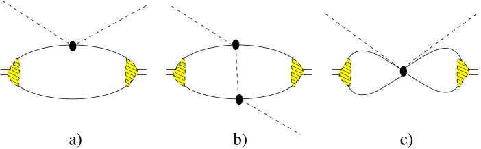
Figure 2: Typical Feynman diagrams for $\pi d$ scattering; shown are the one–body term (a), the double–scattering contribution (b) and a four–nucleon–contact term (c). Solid black dots stand for the $\pi N$ interaction, whereas the hatched area shows the deuteron wave function.

To establish the counting scheme we focus on two–body currents only — how to include one–body currents into the standard scheme is described in Ref. [22]. Thus, in what follows we will compare our two body $\pi NN\to NN\to\pi NN$ operators with the leading two body operator shown in Fig. 2(b). Then it is sufficient to read off the vertex factors for the $\pi NN\to\pi NN$ transitions to identify the order of any given diagram. We therefore estimate $m_{\pi}^{2}/(f_{\pi}^{4}\>q^{2})$ for the diagram (b) of Fig. 2 where $q$ here defines the momentum of intermediate pion. Utilizing Weinbergs counting scheme where all internal momenta are assumed to be of order $m_{\pi}$ we find diagram (b) to be $\mathcal{O}(1)$ — here and in what follows we drop a factor $1/f_{\pi}^{4}$ common to all diagrams to get the order estimate. Power counting gives that the $4N2\pi$ contact term shown in Fig.2 (c) contributes at $\mathcal{O}(\chi^{2})$, where $\chi=m_{\pi}/M_{N}$ is the standard expansion parameter of ChPT with $M_{N}$ for the the nucleon mass. This last contribution comes with a yet unknown coefficient. As such, an estimate for its size provides the theoretical accuracy that a calculation for the $\pi d$ scattering length can have at most. Therefore, assuming naturalness for the strength of the contact term, the theoretical limit of accuracy is of order $\chi^{2}$ which translates into a few percent. Reverting this statement, in order to reach a theoretical accuracy that is comparable to that expected for the experimental value of the $\pi d$ scattering length, all contributions of lower order than $\chi^{2}$ should be evaluated. We will now show that the dispersive corrections contribute to $\mathcal{O}(\chi^{3/2})$.

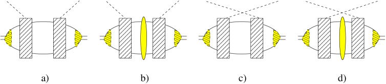
Figure 3: The classes of the hadronic contributions to the dispersive corrections. Diagram (a) and (b) denote the direct and (c) and (d) the crossed terms. The filled ellipse denotes the $NN$ interaction in the intermediate state. The diagrams contributing to the $\pi NN\to NN$ transition to the given order are shown in Fig. 1. The diagrams with emission of pion on the second nucleon are not shown explicitly but taken into account in the calculation.

Transitions of the type $\pi NN\to NN\to\pi NN$ — sketched in Fig. 3 (a) — get contributions from small values of the $NN$ intermediate momentum $q$ ($q\sim m_{\pi}$ or smaller) as well as from large values of $q$ ($q\sim p_{\mbox{thr}}=\sqrt{m_{\pi}M_{N}}$). The latter value refers to the on–shell momentum of the intermediate $NN$ state (or, equivalently, to the threshold initial momentum of the reaction $NN\to NN\pi$). The power counting as given for $NN\to NN\pi$ relates to the latter part of the contribution. It is based on the assignment $p_{\mbox{thr}}/M_{N}\sim\mathcal{O}(\chi^{1/2})$ [16]. To derive the order of the dispersive corrections let us start with diagram $d1$ of Table 1. (See footnote 2 for how to include diagrams of the type $d2$). For this one we find in units of the amplitude for diagram (b) of Fig. 2 (estimated to be $\mathcal{O}(1)$)

$$\left[\left.\left(\frac{m_{\pi}}{f_{\pi}^{3}q}\right)^{2}\frac{1}{m_{\pi}-q^{2}/M_{N}+i\epsilon}\left(\frac{q^{3}}{(4\pi)^{2}}\right)\right]\right/\left(\frac{1}{f_{\pi}^{4}}\right)\sim\left\{\begin{array}[]{ll}\mathcal{O}\left(\chi^{2}\right)&\mbox{for}\,q\sim m_{\pi}\\ \mathcal{O}\left(\chi^{\frac{3}{2}}\right)&\mbox{for}\,q\sim p_{\mbox{thr}}\\ \end{array}\right.$$ (5)

where the first term in the square brackets comes from the $\pi NN\to NN$ transition operator, the second one from the $NN$ propagator in the intermediate state and the last one from the integral measure. To arrive at the estimate for $q\sim p_{\mbox{thr}}$, where the l.h.s of Eq.(5) involves a singularity, we replaced the two–nucleon propagator by the corresponding $\delta$-function term for this estimate should apply to both the real part as well as the imaginary part that emerges from $\pi NN\to NN\to\pi NN$. Furthermore we used $4\pi f_{\pi}\simeq M_{N}$. The small momentum part of the integral is thus of order $\chi^{2}$ and not relevant for this study. That is why dispersive corrections were not considered in the studies of Refs. [3, 4]. However, the part of the integral where $q$ is of the order of $p_{\mbox{thr}}$ is indeed of lower order than $\chi^{2}$ and thus should be considered. It is important to stress that for a consistent understanding of $NN\to NN\pi$ within ChPT it was also necessary to include the large scale $p_{\mbox{thr}}$ explicitly in the power counting [16, 19]. For the imaginary part of the amplitude $\pi NN\to NN\to\pi NN$ we have an experimental value — (3/4)Im$(a_{\pi d})$/Re$(a_{\pi d})\simeq 1/6$, where the factor of 3/4 was introduced since this fraction of the width comes from $\pi d\to NN$. To check the power counting we need some estimate for the real part of the scattering length, which is known to be dominated by the double rescattering term (Fig. 2(b)) and was shown above to be $\mathcal{O}(1)$. Therefore we expect from the above considerations a relative suppression of the imaginary part to the real part of the order of $(m_{\pi}/M_{N})^{3/2}=1/17$. Thus, the hadronic contribution to the imaginary part of the $\pi d$ scattering length is about a factor of 3 larger than predicted by the power counting — a deviation that is tolerable.

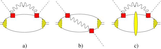
Figure 4: Diagrams contributing to the dispersive corrections from photon–exchange interactions: one–body term (a) and double scattering (b). The filled ellipse denotes the $NN$ interaction in the intermediate state. The solid squares denote the full $\pi N\to\gamma N$ transition amplitude as depicted in Fig. 5.

Since the $NN$ interaction is non–perturbative in diagrams, where a two–nucleon state contributes near on–shell, the full $NN$ interaction should be taken into account — the corresponding diagram is depicted in Fig. 3(b). These are also included in our calculation using the techniques outlined in Ref. [24]. At the same chiral order there is an additional class of contributions — these are the crossed terms shown as diagrams (c) and (d) in Fig. 3. Already in Ref. [27] an evaluation of those diagrams was called for, however, a consistent calculation of the terms that emerge from diagram $ii)$ of Fig. 1 has not been possible so far [10]. Since we work within a consistent field theory no such problem exists. The numerical importance of some crossed diagrams for $\pi d$ scattering was already observed before and referred to as the so-called Jennings mechanism [28]: to understand data measured with tensor polarized deuterons for elastic $\pi d$ scattering at backward angles, a particular crossed pion contribution needs to be included — see also the discussion in Ref. [29]. The order assignment for the crossed diagrams is obvious once one applies the same procedure that leads to the estimate given in (5) — the only necessary change is to switch the sign of $m_{\pi}$ in the $NN$ propagator. Note, in these diagrams the two–nucleon intermediate state is always off–shell in contrast to the $NN$ state in the direct contributions that are expected to receive the dominant contributions from (near) on–shell nucleons. It is therefore surprising that direct and crossed terms appear at the same order. However, one should recall that the chiral expansion is an expansion around the chiral limit. When approaching the chiral limit the intermediate two–nucleon states of both direct and crossed diagrams approach the same kinematical point. Therefore it is natural that they also contribute to the same chiral order for physical pion masses.

A priori there is no rule how to include the electromagnetic contribution to both the real and the imaginary part of the $\pi d$ scattering length (see Fig. 4) into the power counting — the fine structure constant $\alpha$ is clearly an independent parameter. Based on the observation that the electromagnetic and the hadronic contribution to the imaginary part are of the same order of magnitude, we assign the same chiral order to both — as it is often done in chiral perturbation theory studies.

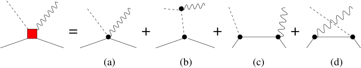
Figure 5: Diagrams contributing to the $\pi N\to\gamma N$ transition operator: Kroll–Rudermann term (a), pion in flight (b) and nucleon s– (c) and u– (d) channel.

3. In this section we present the results of our investigations. We first focus on the hadronic contribution to the dispersive corrections. The results are given in Table 1. Note, for the contributions that involve the $NN$ interaction in the intermediate state we do not give the individual results explicitly. All calculations are done with the CD-Bonn NN potential [30].

First of all we observe that with a value of $4.25\times 10^{-3}\ m_{\pi}^{-1}$ the imaginary part of the scattering length turns out to be very close to the experimental number of $(3/4)$Im$\left(a_{\pi d}^{\mbox{exp}}\right)=(4.7\pm 0.5)\times 10^{-3}\ m_{\pi}^{-1}$ (c.f. Eqs. (1) and (2) and discussion below the latter). This is not too surprising given the good description for the near threshold cross section of $NN\to d\pi$ as reported in Ref. [20]. For the real part on the other hand we observe a striking pattern: although the individual contributions can be quite large, the total sum turns out to be rather small. About 1/3 of the contribution from the direct diagrams of Table 1 gets canceled by the corresponding ones with $NN$ interactions in the intermediate state. This is the same pattern as for the imaginary part — the fact that the latter reduction in the magnitude is natural for processes of the type $NN\to NNx$ was discussed in Ref. [31]. However, about 60 % of the contribution of the direct diagrams of Table 1 is canceled by the corresponding crossed diagrams. As we will see, part of this cancellation is quite natural. When comparing the direct and the crossed diagrams we observe that the two–nucleon propagator in the intermediate state of the former reads $1/(m_{\pi}-q^{2}/M_{N})$ (c.f. Eq. (5)), where $q$ denotes the relevant loop momentum. The corresponding expression for the latter reads $1/(-m_{\pi}-q^{2}/M_{N})$. Thus, for small values of $q$, where the two–nucleon propagator becomes static, one obtains $1/m_{\pi}$ and $-1/m_{\pi}$ respectively, and some contributions of direct and crossed diagrams, specifically d2 and c2, will largely cancel. Note, this cancellation does not mean that the full contribution of each pair of diagrams cancels. The numbers given in the table also contain the contributions from large values of $q$, where such a cancellation does not necessarily occur. Note also that it is the structure of the two nucleon propagator that is responsible for the smallness of diagram d1 as compared to its crossed partner c1. In contrast to diagram c1, the two–nucleon propagator in d1 changes its sign when passing through the point $q^{2}=m_{\pi}M_{N}$ whereas all other terms such as vertex functions, pion propagators, etc., have the same sign throughout the region of integration. Thus, a strong cancellation takes place for the latter and as a result the real part of diagram d1 is much smaller than that of c1. The situation for diagram d3 is different to d1, since also the S-wave deuteron wave function changes sign at $q\sim\sqrt{m_{\pi}M_{N}}$. This leads to a constructive interference of contributions from small and large momenta.

In Fig. 4 we show the diagrams that contribute to the electromagnetic piece of the dispersive contributions. To evaluate the real part of the one–body contribution (diagram (a)) we use the same prescription as used in Ref. [23], namely we subtract the term corresponding to the one–body operator at zero momentum. This removes the leading divergence that in a full calculation needs to be absorbed into the electromagnetic corrections of the $\pi N$ scattering lengths (note, this quantity was recently estimated in Ref. [32]). To ensure gauge invariance the $\pi N\to\gamma N$ amplitude needs to contain all diagrams shown in Fig. 5. However, since for the calculation of the photonic part of the dispersive correction the $\pi N\to\gamma N$ amplitude contributes at threshold, diagrams (c) and (d) are suppressed by one power of $\chi$ as compared to diagrams (a) and (b). Thus, we did not take them into account in this leading order calculation. Because of the same reasoning we neglect also the contributions to the $\pi N\to\gamma N$ amplitude from the $\Delta$ resonance [34]. We calculated the full $\pi d\to\gamma NN\to\pi d$ amplitude in Coulomb gauge. The corresponding propagator is given, e.g., in Ref. [35]. The final result is $(-0.1+i\,1.4)\times 10^{-3}\ m_{\pi}^{-1}$. Again, the imaginary part is sufficiently close to the corresponding experimental value of

Table 1: Hadronic contribution to the real and imaginary part of $a_{\pi d}$ in units of $m_{\pi}^{-1}\times 10^{-3}$. We only show the typical topologies — all permutations are included as indicated by the ellipses. Line code as in Fig. 2.

direct contributions
$d1$		$=$	$0.49$	$+$	$i\,6.68$
$d2$		$=$	$-0.8$	$+$	$i\,0.1$
$d3$		$=$	$-6.02$	$-$	$i\,1.65$
	sum of this group	$=$	$-6.33$	$+$	$i\,5.13$
$d4{-}d6$	corresponding terms with intermediate $NN$ interaction	$=$	$1.96$	$-$	$i\,0.88$
	sum of all direct terms	$=$	$-4.37$	$+$	$i\,4.25$
crossed contributions
$c1$		$=$	$1.83$
$c2$		$=$	$1.37$
$c3$		$=$	$-0.09$
	sum of this group	$=$	$3.11$
$c4{-}c6$	corresponding terms with intermediate $NN$ interaction	$=$	$-0.37$
	sum of all crossed terms	$=$	$2.74$
direct + crossed
	total sum	$=$	$-1.63$	$+$	$i\,4.25$

$(1/4)$Im$\left(a_{\pi d}^{\mbox{exp}}\right)=(1.6\pm 0.2)\times 10^{-3}\ m_{\pi}^{-1}$, whereas the real part is negligible. This conclusion is consistent with that of Ref. [14], where the real part was found to be $-0.2\times 10^{-3}\ m_{\pi}^{-1}$ within a less complete calculation.

4. We now compare our results for the hadronic contributions to other works. The dispersive corrections to $\pi d$ scattering were investigated using Faddeev calculations in Refs. [13]. Since these works considered only those intermediate states that contain at most one pion at a time, all direct diagrams were included. The authors found $-5.6(1.4)\times 10^{-3}\,m_{\pi}^{-1}$ as contribution to the real part — this number was also used in the reanalysis of $\pi d$ scattering in Ref. [14]. This is to be compared with $-4.37\times 10^{-3}\,m_{\pi}^{-1}$ from our work, which agrees to the above result within the uncertainty. Note, the Faddeev equations produce amplitudes that are non–perturbative in the $\pi N$ and the $NN$ interaction simultaneously. Thus, in addition to the direct terms as shown in Table 1 there are many more diagrams included like contributions where the $NN$–pair interacts while there is a pion in flight. However, all those are of higher order in the chiral expansion. The closeness of our result for the direct terms and the corresponding result of Ref. [13] is thus an indication for the convergence of the chiral expansion. Recall that our final result to the real part of $a_{\pi d}$ is smaller because of a cancellation of the mentioned contribution with the crossed diagrams that were not included in Refs. [13].

In Ref. [5] the diagrams $d1$ of Table 1 were evaluated explicitly, besides many others that are difficult to match to our amplitudes. In this work they contribute with $(0.24+i6.0)\times 10^{-3}\,m_{\pi}^{-1}$ to the $\pi d$ scattering length. This number is to be compared to our $(0.49+i6.68)\times 10^{-3}\,m_{\pi}^{-1}$. In Ref. [5] a value of $3/2m_{\pi}$ was used at the $\pi N\to\pi N$ vertex in contrast to the proper $2m_{\pi}$ as derived recently [20]. On the other hand, Ref. [5] includes a (small) isoscalar piece into this vertex — chiral power counting assigns a subleading order to this piece. However, the pattern of the result is the same: a small real part is accompanied by a sizable imaginary part.

Our results for diagrams $d2$ and $c2$ agree to those of Ref. [37], once the same $\pi NN$ coupling constant is used.

Some of the diagrams in Table 1 where included in the phenomenological studies of Refs. [5, 15]. In particular, the second diagrams of d3 and c3 contribute to the so–called SP-interference term (a double scattering diagram, where the first $\pi N\to\pi N$ transition is in an $s$–wave, whereas the second is $p$–wave). In those studies the $p$–wave amplitude was taken from fits to $\pi N$ data and parameterized as a strength parameter times the square of the $\pi N$ relative momentum. Indeed, what appears at the lower nucleon can be regarded as the $\pi N$ scattering in $p$–wave but in the boosted frame. However, this treatment misses an important momentum dependence, since in the boosted frame the nucleon propagator in the intermediate state contains a term $q^{2}/M_{N}$ in the denominator (see Appendix). As a consequence the $p$–wave subamplitude in the phenomenological studies grows quadratically with momentum, even for momenta $q^{2}\sim m_{\pi}M_{N}$ and the full matrix element scales with the wave function at the origin [5], which is theoretically not controlled. On the other hand, in our case this subamplitude goes to a constant leading to a controlled behaviour of the matrix element [7]. This is why those parts of Refs. [5, 15] can not be matched to our results. Based on the arguments given, we call for microscopic calculations, now possible within ChPT, instead of applying the phenomenological techniques.

5. To summarize, in this work we calculated for the first time the absorptive and dispersive corrections to the $\pi d$ scattering length using ChPT. Especially we found for the absorptive part

$$\mbox{Im}(a_{\pi d})=((4.25\pm 1.2)+(1.4\pm 0.4))\times\,10^{-3}\ m_{\pi}^{-1}\$$ (6)

to be compared with the experimental value of

$$\mbox{Im}\left(a_{\pi d}^{\mbox{exp}}\right)=((4.7\pm 0.5)+(1.6\pm 0.2))\times\,10^{-3}\ m_{\pi}^{-1}\ .$$ (7)

In both Eq. (6) as well as Eq. (7) we give the hadronic and electromagnetic contribution separately. We thus find good agreement between theory and experiment for each of the contributions. The theoretical uncertainty is estimated to be of order $2\,m_{\pi}/M_{N}$ in both cases.

For the corresponding dispersive part we get

$$a_{\pi d}^{disp}=-1.7\times 10^{-3}\,m_{\pi}^{-1}\Longrightarrow a_{\pi d}^{disp}/\mbox{Re}\left(a_{\pi d}^{\mbox{exp}}\right)\sim 6.5\%\ .$$ (8)

The number given for $a_{\pi d}^{disp}$ now contains both the hadronic as well as the electromagnetic contribution and for Re($a_{\pi d}^{\mbox{exp}}$) we used Eq. (1). This result is quite small given that the imaginary part of the $\pi d$ scattering length is about 1/4 of the real part. It is difficult to provide a proper estimate for the uncertainty of $a_{\pi d}^{disp}$, since it emerged from a cancellation of individually sizable terms. The most naive method would be to use the uncertainty of order $2\,m_{\pi}/M_{N}$ one has for, e.g., the sum of all direct diagrams to derive a $\Delta a_{\pi d}^{disp}$ of around $1.4\times 10^{-3}\,m_{\pi}^{-1}$, which corresponds to about 6% of $\mbox{Re}\left(a_{\pi d}^{\mbox{exp}}\right)$. However, given that the operators that contribute to both direct and crossed diagrams are almost the same (see Appendix) and that part of the mentioned cancellations is a direct consequence of kinematics, this number for $\Delta a_{\pi d}^{disp}$ is probably too large. A reliable error estimate for $a_{\pi d}^{disp}$ requires an explicit evaluation of the next order contributions.

We showed that the smallness of the dispersive contribution to the real part of the $\pi d$ scattering length is a consequence of efficient cancellations amongst various, individually sizable terms. To gain a better understanding of the real part of the pion-deuteron scattering length, a complete calculation of all isospin-breaking corrections at N(N)LO in the EFT with virtual photons is called for (as also stressed in [9]).

Acknowledgments

Useful discussions with J. Gasser, D. Gotta, E. Oset, D.R. Phillips, A. Rusetsky, A.W. Thomas, and W. Weise are gratefully acknowledged. A. K. and V. B. also thank T.E.O. Ericson for useful discussions. This research is part of the EU Integrated Infrastructure Initiative Hadron Physics Project under contract number RII3-CT-2004-506078, and was supported also by the DFG-RFBR grant no. 05-02-04012 (436 RUS 113/820/0-1(R)) and the DFG SFB/TR 16 ”Subnuclear Structure of Matter”. A. K. and V. B. acknowledge the support of the Federal Program of the Russian Ministry of Industry, Science, and Technology No 02.434.11.7091.

Appendix

In this appendix we present the explicit expressions for the amplitudes depicted in Table 1. Note, in accordance with the definition used for dispersive corrections as well as the power counting, we only keep those amplitudes that contain two–nucleon cuts in time–ordered perturbation theory (TOPT). Especially, we dropped the so–called streched boxes.

Using the same labels as in the table, one finds for the corresponding corrections to the $\pi d$ scattering length

$${a_{\pi d}^{disp}}=-\frac{g_{A}^{2}m_{\pi}^{2}}{6\pi f_{\pi}^{6}(1{+}m_{\pi}/2M_{N})(1{+}q_{0}/2M_{N})}\int\frac{d^{3}q}{(2\pi)^{3}}\frac{q^{2}(\alpha{+}\beta)^{2}}{q_{0}-q^{2}/M_{N}+i\epsilon}\;$$ (A-1)

where

$$\alpha=\left(I_{1}(q)-\frac{3}{2\sqrt{2}}I_{2}(q)\right)\ \mbox{and}\ \beta=\frac{f_{\pi}^{2}}{M_{N}}\left(u(q)+\frac{w(q)}{\sqrt{2}}\right).$$ (A-2)

Here $I_{1}$ and $I_{2}$ are the integrals that correspond to the overlap of the deuteron wave function ($u(q)$ and $w(q)$ for the S- and D-waves, respectively) with the one pion exchange operator

$$I_{1}(q) = -\int\frac{d^{3}p}{(2\pi)^{3}}\frac{(1+({\vec{p}}\cdot{\vec{q}})/q^{2})}{2\omega_{{\vec{p}}+{\vec{q}}}}\left(u(p)+\frac{w(p)}{\sqrt{2}}\right)\left(\frac{1}{P_{1}}+\frac{1}{P_{2}}\right),$$

$$I_{2}(q) = -\int\frac{d^{3}p}{(2\pi)^{3}}\frac{(1-({\vec{p}}\cdot{\vec{q}})^{2}/(p^{2}q^{2}))}{2\omega_{{\vec{p}}+{\vec{q}}}}w(p)\left(\frac{1}{P_{1}}+\frac{1}{P_{2}}\right)$$ (A-3)

where $P_{1}$ and $P_{2}$ correspond to the TOPT components of the pion propagator $P_{1}=q_{0}-\omega_{{\vec{p}}+{\vec{q}}}-(p^{2}+q^{2})/2M_{N}$ and $P_{2}=-\omega_{{\vec{p}}+{\vec{q}}}-(p^{2}+q^{2})/2M_{N}$ with $\omega_{\vec{q}}=\sqrt{{\vec{q}}\>^{2}+m_{\pi}^{2}}$.

The diagrams of Table 1 can be easily matched to the individual terms of Eq. (A-1): type 1 contains $\alpha^{2}$, type 2 contains $\beta^{2}$, whereas the interference terms of type 3 contain $2\alpha\beta$. For the direct terms, labled as $d$ in the table, one needs to take $q_{0}=m_{\pi}$ and for the crossed terms, labled as $c$ in the table, $q_{0}=-m_{\pi}$. All necessary information on how the $NN$ interaction is included in the intermediate state can be found in the Appendix of Ref. [24].

All integrals are evaluated up to a sharp momentum cut–off of 1 GeV. All higher momentum components are to be absorbed in a counter term that is to be included at order $\chi^{2}$ (c.f. discussion in section 2). By enlarging the cut–off by a factor of 20 we checked that the integrals change by less than 10 % — fully in line with the power counting.

References

- [1] P. Hauser et al., Phys. Rev. C 58 (1998) 1869; D. Chatellard et al., Nucl. Phys. A 625 (1997) 855.
- [2] D. Gotta et al., PSI experiment R-06.03; D. Gotta, private communication.
- [3] S. R. Beane, V. Bernard, E. Epelbaum, U.-G. Meißner and D. R. Phillips, Nucl. Phys. A 720 (2003) 399 [arXiv:hep-ph/0206219].
- [4] U.-G. Meißner, U. Raha and A. Rusetsky, Eur. Phys. J. C 41 (2005) 213 [arXiv:nucl-th/0501073].
- [5] M. Döring, E. Oset and M. J. Vicente Vacas, Phys. Rev. C 70 (2004) 045203 [arXiv:nucl-th/0402086].
- [6] M. Pavon Valderrama and E. Ruiz Arriola, Phys. Rev. C 72 (2005) 054002 [arXiv:nucl-th/0504067]; M. P. Valderrama and E. R. Arriola, arXiv:nucl-th/0605078.
- [7] A. Nogga and C. Hanhart, Phys. Lett. B 634 (2006) 210 [arXiv:nucl-th/0511011].
- [8] L. Platter and D. R. Phillips, arXiv:nucl-th/0605024.
- [9] U.-G. Meißner, U. Raha and A. Rusetsky, Phys. Lett.B 639 (2006) 478 [arXiv:nucl-th/0512035].
- [10] A. W. Thomas and R. H. Landau, Phys. Rept. 58 (1980) 121.
- [11] V. C. Highland et al., Nucl. Phys. A 365 (1981) 333.
- [12] K. Brückner, Phys. Rev. 98 (1955) 769.
- [13] I.R. Afnan and A.W. Thomas, Phys. Rev. C10 (1974) 109; D.S. Koltun and T. Mizutani, Ann. Phys. (N.Y.) 109 (1978) 1.
- [14] T. E. O. Ericson, B. Loiseau, A. W. Thomas, Phys. Rev. C 66 (2002) 014005 [arXiv:hep-ph/0009312].
- [15] V.Baru, A. Kudryavtsev, Phys. Atom. Nucl., 60 (1997) 1476.
- [16] T.D. Cohen, J.L. Friar, G.A. Miller and U. van Kolck, Phys. Rev. C 53 (1996) 2661 [arXiv:nucl-th/9512036].
- [17] C. Hanhart, U. van Kolck and G. A. Miller, Phys. Rev. Lett. 85 (2000) 2905 [arXiv:nucl-th/0004033]; C. Hanhart and N. Kaiser, Phys. Rev. C 66 (2002) 054005 [arXiv:nucl-th/0208050].
- [18] B.Y. Park et al., Phys. Rev. C 53 (1996) 1519 [arXiv:nucl-th/9512023]; C. Hanhart, J. Haidenbauer, M. Hoffmann, U.-G. Meißner and J. Speth, Phys. Lett. B 424 (1998) 8 [arXiv:nucl-th/9707029]; V. Dmitrašinović, K. Kubodera, F. Myhrer and T. Sato, Phys. Lett. B 465 (1999) 43 [arXiv:nucl-th/9902048]; S. I. Ando, T. S. Park and D. P. Min, Phys. Lett. B 509 (2001) 253 [arXiv:nucl-th/0003004]; Y. Kim, I. Danchev, K. Kubodera, F. Myhrer and T. Sato, Phys. Rev. C 73 (2006) 025202 [arXiv:nucl-th/0509004].
- [19] C. Hanhart, Phys. Rep. 397 (2004) 155 [arXiv:hep-ph/0311341].
- [20] V. Lensky, V. Baru, J. Haidenbauer, C. Hanhart, A. E. Kudryavtsev and U.-G. Meißner, Eur. Phys. J. A 27 (2006) 37 [arXiv:nucl-th/0511054].
- [21] D. Koltun and A. Reitan, Phys. Rev. 141 (1966) 1413.
- [22] S. Weinberg, Phys. Lett. B 295 (1992) 114.
- [23] V. Baru, C. Hanhart, A. E. Kudryavtsev and U.-G. Meißner, Phys. Lett. B 589 (2004) 118 [arXiv:nucl-th/0402027].
- [24] V. Lensky, V. Baru, J. Haidenbauer, C. Hanhart, A. E. Kudryavtsev and U.-G. Meißner, Eur. Phys. J. A 26 (2005) 107 [arXiv:nucl-th/0505039]. arXiv:nucl-th/0505039.
- [25] B. Borasoy and H. W. Grießhammer, Int. J. Mod. Phys. E 12 (2003) 65.
- [26] S. R. Beane and M. J. Savage, Nucl. Phys. A 717 (2003) 104 [arXiv:nucl-th/0204046].
- [27] D. J. Thouless, in: Proc. Phys. Soc. (London) 69 (1956) 280.
- [28] B.K. Jennings, Phys. Lett. B 205 (1988) 187.
- [29] H. Garcilazo and T. Mizutani, NN Systems, World Scientific, Singapore, 1990.
- [30] R. Machleidt, Phys. Rev. C 63 (2001) 024001 [arXiv:nucl-th/0006014].
- [31] C. Hanhart and K. Nakayama, Phys. Lett. B 454, 176 (1999) [arXiv:nucl-th/9809059].
- [32] T. E. O. Ericson and A. N. Ivanov, Phys. Lett. B 634 (2006) 39.
- [33] J. Gasser, A. Rusetsky and I. Scimemi, Eur. Phys. J. C 32 (2003) 97 [arXiv:hep-ph/0305260].
- [34] H. W. Fearing, T. R. Hemmert, R. Lewis and C. Unkmeir, Phys. Rev. C 62 (2000) 054006 [arXiv:hep-ph/0005213].
- [35] V. B. Berestetsky, E. B. Lifshitz and L. P. Pitaevsky, “Quantum Electrodynamics,” Oxford, Uk: Pergamon (1982) (Course Of Theoretical Physics, 4).
- [36] R. M. Rockmore, Phys. Lett. B 356 (1995) 153.
- [37] V. Tarasov, V. Baru, A. Kudryavtsev, Phys. of Atom. Nucl., 63 (2000) 801.