Chiral effective theory predictions for deuteron form factor ratios at low $Q^{2}$

Daniel R. Phillips
Department of Physics and Astronomy, Ohio University, Athens, OH 45701
Department of Natural Sciences, Chubu University, 1200 Matsumoto-cho, Kasugai, Aichi 487-8501, JAPAN
Email: phillips@phy.ohiou.edu

We use chiral effective theory ($\chi$ET) to predict the deuteron form factor ratio $G_{C}/G_{Q}$ as well as ratios of deuteron to nucleon form factors. These ratios are calculated to next-to-next-to-leading order. At this order the chiral expansion for the $NN$ isoscalar charge operator (including consistently calculated $1/M$ corrections) is a parameter-free prediction of the effective theory. Use of this operator in conjunction with NLO and NNLO $\chi$ET wave functions produces results that are consistent with extant experimental data for $Q^{2}<0.35$ GeV². These $\chi$ET wave functions predict a deuteron quadrupole moment $G_{Q}(Q^{2}=0)=0.278$–$0.282~{}{\rm fm}^{2}$—with the variation arising from short-distance contributions to this quantity. The variation is of the same size as the discrepancy between the theoretical result and the experimental value. This motivates the renormalization of $G_{Q}$ via a two-nucleon operator that couples to quadrupole photons. After that renormalization we obtain a robust prediction for the shape of $G_{C}/G_{Q}$ at $Q^{2}<0.3~{}{\rm GeV}^{2}$. This allows us to make precise, model-independent predictions for the values of this ratio that will be measured at the lower end of the kinematic range explored at BLAST. We also present results for the ratio $G_{C}/G_{M}$.

PACS nos.: 12.39.Fe, 25.30.Bf, 21.45.+v

1 Introduction

The static electromagnetic properties of deuterium provide interesting information on the dynamics at work within the nucleus. The fact that deuterium’s charge is one teaches us little other than the validity of charge conservation in the nuclear system, but that its magnetic moment $\mu_{d}\neq\mu_{n}+\mu_{p}$ and that it has of a non-zero quadrupole moment are facts which played an important role in establishing that non-central components of the $NN$ potential are at work within the deuterium nucleus.

The most accurate value for the deuteron quadrupole moment comes from a molecular physics experiment [1, 2]. It is:

$$Q_{d}=0.2859(3)~{}{\rm fm}^{2}.$$ (1)

Meanwhile the best determination of $\mu_{d}$ comes from the spectroscopy of the deuterium atom. It is [3]:

$$\mu_{d}=0.8574382284(94)~{}\mu_{N}.$$ (2)

But elastic electron scattering from deuterium—provided the one-photon-exchange approximation is valid—probes M1 and E2 responses for (virtual) photons that have a finite three-momentum ${\bf q}$. The relevant form factors are related to Breit-frame matrix elements of the two-nucleon four-current $J_{\mu}$ via

$$G_{M} = -\frac{1}{\sqrt{2\eta}|e|}\left\langle 1\left|J^{+}\right|0\right\rangle,$$ (3)

$$G_{Q} = \frac{1}{2|e|\eta M_{d}^{2}}\left(\left\langle 0\left|J^{0}\right|0\right\rangle-\left\langle 1\left|J^{0}\right|1\right\rangle\right).$$ (4)

These, together with the charge form factor, $G_{C}$:

$$G_{C}=\frac{1}{3|e|}\left(\left\langle 1\left|J^{0}\right|1\right\rangle+\left\langle 0\left|J^{0}\right|0\right\rangle+\left\langle-1\left|J^{0}\right|-1\right\rangle\right),$$ (5)

provide a complete set of invariant functions for the description of the deuterium four-current that interacts with the electron’s current in this approximation. In Eqs. (3)–(4) we have labeled the deuteron states by the projection of the deuteron spin along the direction of the three-vector ${\bf p}_{e}^{\prime}-{\bf p}_{e}\equiv{\bf q}$, and $\eta\equiv Q^{2}/(4M_{d}^{2})$, with $Q^{2}=|{\bf q}|^{2}$ since we are in the Breit frame. We can then calculate the deuteron structure functions:

$$A = G_{C}^{2}+\frac{2}{3}\eta G_{M}^{2}+\frac{8}{9}\eta^{2}M_{d}^{4}G_{Q}^{2},$$ (6)

$$B = \frac{4}{3}\eta(1+\eta)G_{M}^{2}.$$ (7)

In terms of $A$ and $B$ the one-photon-exchange interaction yields a lab. frame differential cross section for electron-deuteron scattering

$$\frac{d\sigma}{d\Omega}=\frac{d\sigma}{d\Omega}_{\rm NS}\left[A(Q^{2})+B(Q^{2})\tan^{2}\left(\frac{\theta_{e}}{2}\right)\right],$$ (8)

Here $\theta_{e}$ is the electron scattering angle, and $\frac{d\sigma}{d\Omega}_{\rm NS}$ is the (one-photon-exchange) cross section for electron scattering from a point particle of charge $|e|$ and mass $M_{d}$. The form factors defined in Eqs. (3)–(5) are related to the static moments of the nucleus by:

$$G_{C}(0) = 1,$$ (9)

$$G_{Q}(0) = Q_{d},$$ (10)

$$G_{M}(0) = \mu_{d}\frac{M_{d}}{M},$$ (11)

with $M$ the nucleon mass. For recent reviews of experimental and theoretical work on elastic electron-deuteron scattering see Refs. [4, 5, 6].

From Eq. (8) it is already clear that measurements of the differential cross section alone cannot yield uncorrelated information on all three form factors. To measure $G_{Q}$, $G_{M}$, and $G_{C}$ in a model-independent way one must obtain data with polarized deuterium targets or polarized electron beams. A new set of measurements of polarization observables in electron-deuteron scattering will soon be available from the data set obtained at the Bates Large-Acceptance Spectrometer Toroid (BLAST). There polarized electrons of energy 850 MeV circulated in the Bates ring and were scattered from an internal target containing polarized deuterium. The significant amount of beam on target (3 million Coulombs since late 2003), and high degree of beam and target polarization achieved at BLAST, means that we anticipate data on electron-deuteron polarization observables that is more precise than that derived from any previous measurement.

The electron beam circulating in the Bates ring was roughly 70% polarized, and the deuterium target employed could operate in both a vector-polarized and tensor-polarized mode. This gives access to all of the elastic electron scattering deuterium structure functions. Prominent among these are $t_{11}$, the vector analyzing power, and $t_{20}$, the tensor analyzing power. They are related to the form factors defined above by [5]

$$t_{20}=-\sqrt{2}\frac{x(x+2)+\frac{1}{2}y^{2}(1+2\varepsilon)}{1+2(x^{2}+y^{2}(1+2\varepsilon))};\quad t_{11}=2\sqrt{\varepsilon}y\frac{1+\frac{x}{2}}{1+2(x^{2}+y^{2}(1+2\varepsilon))},$$ (12)

where the ratios $x$ and $y$ are:

$$x = \frac{2}{3}\,\eta\,\frac{G_{Q}M_{d}^{2}}{G_{C}},$$ (13)

$$y = \sqrt{\frac{\eta}{3}}\frac{G_{M}}{G_{C}},$$ (14)

and $\varepsilon=(1+\eta)\tan^{2}\left(\frac{\theta_{e}}{2}\right)$. Therefore measurements of $t_{11}$ and $t_{20}$ should facilitate the extraction of the ratios $G_{M}/G_{C}$ (which at the $Q^{2}$’s we will consider here mainly affects $t_{11}$) and $G_{Q}/G_{C}$ (which mainly affects $t_{20}$). In this paper we provide predictions for these ratios which are based on chiral effective theory ($\chi$ET).

This approach (for reviews see Refs. [7, 8, 9, 10]) is based on the use of a chiral expansion for the physics of the two-nucleon system. In the formulation suggested by Weinberg [11, 12, 13], the $\chi$ET treatment of the $NN$ system is based on a systematic chiral and momentum expansion for the two-nucleon-irreducible kernels of the processes of interest. In particular, wave functions are computed using an $NN$ potential expanded up to a given order in the small parameter:

$$P\equiv\frac{p,m_{\pi}}{\Lambda}$$ (15)

where $p$ is the momentum of the nucleons and $\Lambda$ is the breakdown scale of the theory. For electron-deuteron scattering the other two-nucleon-irreducible kernel that must be calculated is the deuteron current operator $J_{\mu}$. We also expand this object as:

$$J_{\mu}=e\sum_{i=1}^{\infty}\xi_{i}\frac{1}{\Lambda^{i-1}}{\cal O}_{\mu}^{(i)},$$ (16)

where the operator ${\cal O}_{\mu}^{(i)}$ contains $i-1$ powers of the small parameter $P$, which now includes the momentum transfer to the nucleus, $q$, as one of the small scales in the numerator. For chiral effective theories without an explicit Delta degree of freedom $\Lambda$ will in general be $M_{\Delta}-M$, but in electron-deuteron elastic scattering the $\Delta N$ intermediate state is not allowed and so $\Lambda$ will be larger, $\Lambda\,\raisebox{-3.44444pt}{$\stackrel{{\scriptstyle\textstyle>}}{{\sim}}$ }2(M_{\Delta}-M)$.

The $NN$ potential has now been computed up to $O(P^{2})$ [14, 15], $O(P^{3})$ [14, 15, 16] and $O(P^{4})$ [17, 18]. In this paper we will employ wave functions computed using the next-to-leading order [NLO=$O(P^{2})$], next-to-next-to-leading order [NNLO=$O(P^{3})$] and N³LO potentials [$O(P^{4})$] developed in Ref. [18]. These potentials are regularized in two different ways: first, spectral-function regularization (SFR) at a scale $\bar{\Lambda}$ [19], is applied to the two-pion contributions. Then, after the SFR potential $V_{ll^{\prime}}^{sj}(p,p^{\prime})$ is obtained in a particular $NN$ partial wave, it is multiplied by a regulator function $f$, so that the Lippmann-Schwinger equation can be straightforwardly solved:

$$V_{ll^{\prime}}^{sj}(p,p^{\prime})\rightarrow f(p)V_{ll^{\prime}}^{sj}(p,p^{\prime})f(p^{\prime})\quad\mbox{with}\quad f(p)=\exp\left(-\frac{p^{6}}{\Lambda^{6}}\right).$$ (17)

There have been questions raised as to the consistency of the wave functions computed in this way [20, 21, 22, 23, 24, 25]. Partly because of these questions we will, for comparison, also present results for electron-deuteron matrix elements using the form (16) for the current operator, and wave functions derived from the Nijm93 [26] or CD-Bonn [27] potentials, as well as potentials with one-pion exchange at long range and a square well and surface delta function of radius $R$ [28]. We stress that such calculations are not chirally consistent. However, common features of deuteron observables that can be identified within calculations that use these different types of wave functions—chiral effective theory, potential models, and one-pion-exchange tails—should be independent of the details of physics at ranges $\ll 1/m_{\pi}$ in deuterium, and so should not be sensitive to any subtleties pertaining to the renormalization of the $\chi$ET.

The operators ${\cal O}_{\mu}^{(i)}$ and the coefficients $\xi_{i}$ in Eq. (16) are constructed according to the counting rules and Lagrangian of heavy-baryon chiral perturbation theory (HB$\chi$PT), which is reviewed in Ref. [30]. Here the results we will present for $G_{C}$ and $G_{Q}$ include all contributions to $J_{\mu}$ up to chiral order $eP^{3}$. This is the next-to-next-to-leading order (NNLO) for these quantities. Calculations of electron-deuteron scattering with the NNLO $\chi$ET operator were already considered in Ref. [31], which improved upon results with the $O(eP^{2})$ operator in Ref. [32] and the $O(e)$ results of Ref. [28]. However, as was already observed in Ref. [31] and is reiterated below, calculation of the quadrupole combination of matrix elements at NNLO does not reproduce the experimental value of $Q_{d}$ to the accuracy one would expect at that order. We identify the cause of this as short-distance two-body contributions to $J_{0}$ of natural size (i.e. with $\xi_{i}\sim 1$) through which quadrupole photons induce an $L=0\rightarrow L=0$ transition in the $S=1$ deuteron state [28, 29]. We use the operator induced by these short-distance contributions to renormalize the deuteron quadrupole moment, and hence the form factor $G_{Q}$. We also provide results for $G_{M}$ up to NLO. Not surprisingly, $G_{M}$ at NLO proves more sensitive to short-distance physics than does the renormalized $G_{Q}$.

Throughout this work we will use the factorization of nucleon structure employed in Ref. [31] in order to include the effects of finite nucleon size in the calculation. There it was shown that the chiral expansion for the ratios:

$$\frac{G_{C}}{G_{E}^{(s)}}\quad\mbox{and}\quad\frac{G_{Q}}{G_{E}^{(s)}}\quad\mbox{and}\quad\frac{G_{M}}{G_{M}^{(s)}},$$ (18)

with $G_{E}^{(s)}$ and $G_{M}^{(s)}$ the isoscalar single-nucleon electric and magnetic form factors, is better behaved than the chiral expansion for $G_{C}$, $G_{Q}$, and $G_{M}$ themselves. The ratios (18) allow us to focus on the ability of the chiral expansion to describe deuteron structure, and we will employ the $\chi$ET results for the ratios in our efforts to predict BLAST’s results for polarized electron scattering from a deuterium target. We note that, up to the order we work to here, our predictions for $G_{C}/G_{Q}$ are independent of the manner in which we include nucleon structure in the calculation. Our invoking the factorization of nucleon structure in the electron-deuteron matrix elements plays no role in our predictions for $G_{C}/G_{Q}$.

The chiral perturbation theory for this calculation was laid out in Refs. [31, 32], and so here we merely summarize the pertinent features of the chiral expansion for the deuteron currents in Section 2. However, in doing so we find that we must address the issue of how to calculate the corrections to this ratio that have coefficients which are fixed by low-energy Lorentz invariance. We deal with this problem in Section 3, by recalling results of Friar, Adam et al., and Arenhövel et al., which show that such corrections can be calculated unambiguously, as long as they are included consistently in both the $NN$ potential and the current operator. Then, in Section 4 we discuss effects in the $J_{0}$ operator beyond $O(eP^{3})$, and explain how we will estimate their impact on $G_{C}$ and $G_{Q}$. In particular, we write down an operator that represents the effects of physics at mass scales above 1 GeV on $G_{Q}$, and can repair the discrepancy between the experimental value of $Q_{d}$ and our predictions for $G_{Q}(0)$. We also discuss how to estimate the remaining uncertainty in our results. Then, in Section 5 we present results for $G_{C}$, $G_{Q}$, and the ratio $G_{C}/G_{Q}$. We show that the shape of $G_{Q}$ can be predicted in a model-independent way for $Q^{2}<0.3$ GeV², but the uncertainty in the ratio $G_{C}/G_{Q}$ is sizeable at $Q^{2}\approx 0.4$ GeV². Finally, in Section 6 we present results for $G_{C}/G_{M}$, and in Section 7 we summarize and provide an outlook.

2 The deuteron current

We now discuss the charge and current operators in turn. Such a decomposition is, of course, not Lorentz invariant, so here we make this specification in the Breit frame.

2.1 Deuteron charge

The vertex from ${\cal L}_{\pi N}^{(1)}$ which represents an $A_{0}$ photon coupling to a point nucleon gives the leading-order (LO) contribution to $J_{0}$ as depicted in Fig. 1(a). At $O(eP^{2})$ this is corrected by insertions in ${\cal L}_{\pi N}^{(3)}$ that generate the nucleon’s isoscalar charge radius. This gives a result for $J_{0}$ through $O(eP^{2})$:

$$J_{0}^{(2)}=|e|\left(1-\frac{1}{6}\langle r_{Es}^{2}\rangle Q^{2}\right)+j_{0}^{(1/M^{2})}({\bf q})$$ (19)

with $j_{0}^{(1/M^{2})}({\bf q})$ the “relativistic” corrections to the single-nucleon charge operator. These contributions have fixed coefficients that are determined by the requirements of Poincaré invariance. Since these coefficients scale as $1/M^{2}$ this particular set of $O(eP^{2})$ contributions are generally smaller than one would estimate given the formula (15) for the parameter $P$. These “relativistic” corrections can be calculated by writing down a $J_{0}$ operator that, when inserted between deuteron wave functions calculated in the two-nucleon center-of-mass frame, yields results for the matrix elements that are Lorentz covariant up to the order to which we work. To do this we employ the formalism of Adam and Arenhövel, as described in Ref. [33].

Figure 1: Diagrams representing the leading contribution to the deuteron charge operator [(a)], the leading two-body contribution to $J_{0}$ [(b)], and the dominant short-distance piece [(c)]. Solid circles are vertices from ${\cal L}_{\pi N}^{(1)}$, and the shaded circle is the vertex from ${\cal L}_{\gamma\pi N}^{(2)}$.

Meanwhile the only contribution at $O(eP^{3})$, or NNLO, comes from the tree-level two-body graph shown in Fig. 1(b). In HB$\chi$PT the relevant single-nucleon photo-pion vertex arises as a consequence of the Foldy-Wouthuysen transformation which generates a term in ${\cal L}^{(2)}$. Straightforward application of the Feynman rules for the relevant pieces of the HB$\chi$PT Lagrangian gives the result for this piece of the deuteron current [31]:

$$\langle{\bf p}^{\prime}|J_{0}^{(3)}({\bf q})|{\bf p}\rangle=\tau_{1}^{a}\tau_{2}^{a}\,\,\frac{|e|g_{A}^{2}}{8f_{\pi}^{2}M}\,\,\left[\frac{\sigma_{1}\cdot{\bf q}\,\sigma_{2}\cdot({\bf p}-{\bf p}^{\prime}+{\bf q}/2)}{m_{\pi}^{2}+({\bf p}-{\bf p}^{\prime}+{\bf q}/2)^{2}}+(1\leftrightarrow 2)\right],$$ (20)

where ${\bf p}$ and ${\bf p}^{\prime}$ are the (Breit-frame) relative momenta of the two nucleons in the initial and final-state respectively (see Ref. [34] for a much earlier derivation).

Thus we now have a result for the deuteron’s charge operator which can be summarized as:

$$\langle{\bf p}^{\prime}|J_{0}({\bf q})|{\bf p}\rangle=\left[|e|\left(1-\frac{1}{6}\langle r_{Es}^{2}\rangle Q^{2}\right)+j_{0}^{(1/M^{2})}({\bf q})\right]\delta^{(3)}(p^{\prime}-p-q/2)+\langle{\bf p}^{\prime}|J_{0}^{(3)}({\bf q})|{\bf p}\rangle+O(eP^{4}).$$ (21)

However, it was shown in Ref. [31] that the parameterization (19) of the nucleon’s isoscalar charge distribution breaks down at $|{\bf q}|\approx 300$ MeV. In order to avoid this difficulty we observe that the result (21) may be recast, up to the order to which we work, as:

$$\langle{\bf p}^{\prime}|J_{0}({\bf q})|{\bf p}\rangle=\left[\left(|e|+j_{0}^{(1/M^{2})}({\bf q})\right)\delta^{(3)}(p^{\prime}-p-q/2)+\langle{\bf p}^{\prime}|J_{0}^{(3)}({\bf q})|{\bf p}\rangle\right]G_{E}^{(s)}(Q^{2})+O(eP^{4}),$$ (22)

with $G_{E}^{(s)}(Q^{2})$ the complete one-loop HB$\chi$PT result for the nucleon’s isoscalar electric form factor [35]. This means that we can write a result that is independent of $\chi$PT’s difficulties in describing nucleon structure if we focus on the ratio of $\langle{\bf p}^{\prime}|J_{0}({\bf q})|{\bf p}\rangle$ to $G_{E}^{(s)}(Q^{2})$. We will then use experimental data , in particular the parameterization of Mergell et al. [37], for $G_{E}^{(s)}(Q^{2})$ in all computations we present below. This use of experimental data for the single-nucleon matrix element that appears in Eq. (22) allows us to focus on how well the $\chi$ET is describing deuteron structure, since it removes the nucleon-structure issues from the computation of the deuterium matrix element. Our technique to achieve this is rigorous, up to the chiral order to which we work here. The ratio $G_{C}/G_{Q}$ can also be computed independent of nucleon-structure issues, as is made clear by a brief examination of Eq. (22), together with the definitions (5) and (4).

2.2 Deuteron three-current

The counting for the isoscalar three-vector current ${\bf J}$ was already considered in detail by Park and collaborators [38]. ${\bf J}$ begins at $O(eP)$, but at $O(eP^{3})$ there are finite-size and relativistic corrections, which are suppressed by two powers of $P^{2}$. This is the highest order we will calculate $G_{M}$ to here, and at this order, using factorization we have:

$$\langle{\bf p}^{\prime}|{\bf J}^{(3)}|{\bf p}\rangle=[|e|({\bf p}+{\bf q}/2)/M+i\mu_{S}{\bf\sigma}\times{\bf q}+{\bf J}^{(1/M^{2})}({\bf q})]G_{M}^{(s)}(Q^{2})\delta^{(3)}(p^{\prime}-p-q/2).$$ (23)

with ${\bf p}-{\bf q}/4$ is the momentum of the struck nucleon, and $\mu_{S}$ is the isoscalar magnetic moment of the nucleon, whose value we take to be $\mu_{S}=0.88|e|/(2M)$.

At $O(eP^{4})$ [NNLO] two kinds of magnetic two-body current enter the calculation. One is short-ranged, and one is of pion range [38, 29, 39, 40, 32]. Each of them has an undetermined coefficient. In principle those coefficients should be fit to data (e.g. the deuteron magnetic moment, which is not exactly reproduced by the current ${\bf J}$ and the wave functions employed here) and the low-$Q^{2}$ shape of the form factor.

3 Unitary equivalence and the consistent treatment of $1/M$ corrections

In this section we discuss the constraints imposed by Poincaré invariance—or the low-energy manifestations thereof—on the Breit-frame isoscalar $NN$ charge operator. Recall that in HB$\chi$PT $\langle{\bf p}^{\prime}|J_{0}^{(3)}({\bf q})|{\bf p}\rangle$ arises from a piece of ${\cal L}_{\pi N}^{(2)}$ that has a fixed coefficient obtained via a Foldy-Wouthuysen transformation. Therefore this piece of the charge operator is a low-energy consequence of Lorentz covariance of $\langle M^{\prime}|J_{\mu}|M\rangle$. As such the contribution (20) should be computed in a manner consistent with that used to derive the $1/M^{2}$ corrections to the one-pion exchange part of the $NN$ potential. Those $1/M^{2}$ corrections can be obtained from the chiral Lagrangian— specifically from the $1/M$ pieces in ${\cal L}_{\pi N}^{(2)}$ and the $1/M^{2}$ pieces in ${\cal L}_{\pi N}^{(3)}$. But the relevant operators involve the energy of the individual nucleons, and so it is not immediately obvious how to convert them to contributions to an energy-independent quantum-mechanical potential. In fact, in the 1970s and 1980s many techniques were developed by which quantum-mechanical operators could be obtained from a relativistic quantum field theory [33, 41, 42]. In all of these techniques there was freedom in choosing whether (and if so, which) nucleon lines to put on shell, as well as freedom in how to include meson retardation. As we shall see, the choices made with respect to these two issues have an impact on the form of the operators (both $V$ and $J_{0}$) that are obtained. Ultimately though, as long as operators and potentials are derived in a consistent way, the different choices are related by unitary transformations that leave matrix elements unaffected [41, 42, 43].

That unitary transformation is labeled by two parameters: $\nu$, which parameterizes the energy, $k_{0}$, of the exchanged pion via

$$k_{0}^{2}=\left(1-2\nu\right)\frac{(p^{\prime 2}-p^{2})^{2}}{4M^{2}},$$ (24)

where $p^{\prime}$ ($p$) is the length of the relative three-momentum vector of the $NN$ system after (before) the meson exchange; and $\beta$, which denotes a choice for the change in the nucleons’ energy after absorption of the pion [41]:

$$(p_{0}^{\prime}-p_{0})_{1,2}=(1-2\beta)\frac{p^{\prime 2}-p^{2}}{2M}.$$ (25)

Note that in quantum mechanics energy is not conserved at each vertex, and so $(p_{0}^{\prime}-p_{0})_{1}=k_{0}=-(p_{0}^{\prime}-p_{0})_{2}$ need not necessarily hold. Indeed, it turns out that since we are in the $NN$ c.m. frame the difference $p_{0}^{\prime}-p_{0}$ is the same for both nucleons once an energy shell is chosen. The full expression for the $1/M^{2}$ corrections to the one-pion-exchange potential in the case of arbitrary $\beta$ and $\nu$ can be found in Ref. [41]. The main result for our purposes here is that if $\beta=\frac{1}{4}$ then the potential takes the form:

$$\langle{\bf p}^{\prime}|V^{(1\pi)}|{\bf p}\rangle=-\tau_{1}^{a}\tau_{2}^{a}\frac{g_{A}^{2}}{4f_{\pi}^{2}}\frac{\sigma_{1}\cdot({\bf p}^{\prime}-{\bf p})\sigma_{2}\cdot({\bf p}^{\prime}-{\bf p})}{({\bf p}^{\prime}-{\bf p})^{2}+m_{\pi}^{2}}\left(1-\frac{p^{\prime 2}+p^{2}}{2M^{2}}+O\left(\frac{1}{M^{4}}\right)\right).$$ (26)

This is the one-pion-exchange potential used in the N³LO computation of Ref. [18]. (Corrections to “leading” two-pion exchange diagrams that are suppressed by $1/M$ are also included there, but are associated with pieces of the $J_{0}$ which are of higher order than we work to here.) The computation of Ref. [27] employed the form for $\langle{\bf p}^{\prime}|V^{(1\pi)}|{\bf p}\rangle$ that corresponds to $\beta=0$. All other potentials we discuss here (including the NNLO and NLO ones used in Ref. [18]) employed the non-relativistic form of OPE, i.e. the result (26), but without the additional factor in the round brackets. Meanwhile, all of the potentials we have used neglect retardation, which means they have set $\nu=\frac{1}{2}\Leftrightarrow k_{0}=0$.

Consistent reduction of the contributions to the deuteron charge operator then leads to a more general result for diagram Fig. 1(b) than that given in Eq. (20) [41]:

$$\langle{\bf p}^{\prime}|J_{0}^{(3)}({\bf q})|{\bf p}\rangle=\tau_{1}^{a}\tau_{2}^{a}\,\,\frac{|e|g_{A}^{2}}{8f_{\pi}^{2}M}\,\,\left[(1-\beta)\frac{\sigma_{1}\cdot{\bf q}\,\sigma_{2}\cdot({\bf p}-{\bf p}^{\prime}+{\bf q}/2)}{m_{\pi}^{2}+({\bf p}-{\bf p}^{\prime}+{\bf q}/2)^{2}}\right.$$

$$\qquad-\frac{1-\nu}{2}\left.\frac{\sigma_{1}\cdot({\bf p}-{\bf p}^{\prime}+{\bf q}/2)\,\sigma_{2}\cdot({\bf p}-{\bf p}^{\prime}+{\bf q}/2)\,\,\,{\bf q}\cdot({\bf p}-{\bf p}^{\prime}+{\bf q}/2)}{[m_{\pi}^{2}+({\bf p}-{\bf p}^{\prime}+{\bf q}/2)^{2}]^{2}}+(1\leftrightarrow 2)\right].$$

(27)

In Eq. (20) we obtained the result for the $O(eP^{3})$ piece of the charge operator that corresponds to $\beta=0$ and $\nu=1$, because the field-theoretic manipulations used to arrive at Eq. (20) assume that the fields represent physical particles, i. e. they are on-shell. The result (27) may be obtained from Eq. (20) by applying a unitary transformation [41, 42]:

$$J_{0}^{(3)}(\beta,\nu)=U^{\dagger}(\beta,\nu)J_{0}^{(3)}(0,1)U(\beta,\nu),$$ (28)

where the form of $U$ can be found in the original papers. The same unitary transformation generates consistent $1/M^{2}$ corrections to the one-pion-exchange part of the $NN$ potential:

$$V_{\rm OPE}(\beta,\nu)=U^{\dagger}(\beta,\nu)V_{\rm OPE}(0,1)U(\beta,\nu),$$ (29)

including the form (26) if the choice $\beta=\frac{1}{4}$, $\nu=\frac{1}{2}$ is adopted. This is not consistent with the choice made in obtaining Eq. (20) in Ref. [31] because the $NN$ potential of Ref. [18] was computed using the Okubo formalism developed in Ref. [44].

In Ref. [18] this issue of the choice made for $\beta$ and $\nu$ does not arise until the N³LO potential is derived, because in that paper, and in the earlier Refs. [44, 15], Epelbaum et al. chose to count $M\sim\Lambda^{2}$. In doing this they were adhering to Weinberg’s original argument as to why it is the two-nucleon-irreducible kernel—and not the $NN$ amplitude itself—which admits a chiral expansion. $NN$ intermediate states introduce factors of $M$ in the amplitude for loop graphs, and if $M\sim\Lambda^{2}$ then the $n$th iterate of the one-pion-exchange potential is the same order as one-pion exchange itself [11, 12]. However, in Ref. [21] the need to iterate the one-pion-exchange potential to all orders was established without any reference to counting $M\sim\Lambda^{2}$, being justified instead by the singular, and attractive, nature of the $NN$ force (see also Ref. [25]). Therefore, while it is true that corrections to the $NN$ potential which are suppressed by powers of $1/M$ are often smaller than, e.g. those arising from excitation of the Delta(1232), in discussing electron-deuteron scattering we will consider a regime in which $q/M$ can be sizeable. Therefore we follow the original HB$\chi$PT counting and take $M\sim\Lambda$. As we shall see, this counting is supported by the fact that the contribution (20) plays a significant, but not excessive, role in the deuteron charge and quadrupole form factors.

If we count $M\sim\Lambda$ the dilemma presented by the inconsistency between $V$ and $J_{0}$ arises already at $O(eP^{3})$. A way out of this dilemma is provided by Eqs. (28) and (29). They guarantee that we will obtain the same result (up to $O(p^{4}/M^{4})$ corrections) for deuteron matrix elements $\langle M^{\prime}|J_{0}|M\rangle$, regardless of what choices for $\beta$ and $\nu$ we make when constructing the operators $V$ and $J_{0}$ from the chiral effective field theory, provided that we consistently include the $O(p^{2}/M^{2})$ pieces of the potential $V$ and the $O(eP^{3})$ pieces of the operator $J_{0}$. Therefore in order to be consistent with the calculation of the $1/M^{2}$ corrections to $V_{\rm OPE}$ in Ref. [18] we must adopt the choice $\beta=\frac{1}{4}$ in the formula (27) for $J_{0}^{(3)}$. If we do this, and also make sure to calculate one-pion exchange according to the formula (26), then our results for matrix elements of the deuteron charge operator will incorporate the low-energy consequences of Lorentz invariance, up to corrections of $O(p^{4}/M^{4})$ (higher order than we consider here). Note that the CD-Bonn potential is a different case, since the use of a pseudoscalar $\pi NN$ coupling means that there we have $\beta=0$. Therefore in that case, and only in that case, we have used the expression (20) for the first part of $J_{0}^{(3)}$, with no modification by the factor of $\frac{3}{4}$ that must be present if $V^{(1\pi)}$ is constructed with $\beta=\frac{1}{4}$.

This still leaves us with the issue of how the $p^{2}/M^{2}$ corrections in the one-pion exchange potential (26) and the $p^{2}/M^{2}$ corrections to the nucleon kinetic energy operator are to be accounted for in the calculations using the NNLO and NLO wave functions of Ref. [18] (or included in calculations with the Nijm93 wave function of Ref. [26] or the wave functions of Ref. [28]). The original calculations of these wave functions did not include such effects, but since we count $M\sim\Lambda$ here, we need to include them in order to have a consistent calculation of $G_{C}$ and $G_{Q}$ to $O(eP^{3})$.

Starting from the Kamada-Glöckle transformation [45], we show in Appendix A the major part of these effects can be included by making changes to the short-distance pieces of the $NN$ potential, and using a slightly modified wave function $\psi$ in the computation of $G_{C}$, $G_{Q}$, and $G_{M}$. That wave function is related to the original non-relativistic wave function $\tilde{\psi}$ obtained in Ref. [18] by [45]:

$$\psi(p)=\sqrt{\frac{M}{\sqrt{M^{2}+p^{2}}}}\left(\frac{2M}{M+\sqrt{M^{2}+p^{2}}}\right)^{1/4}\tilde{\psi}\left(\sqrt{2M\sqrt{M^{2}+p^{2}}-2M^{2}}\right).$$ (30)

The solution of the non-relativistic Schrödinger equation for the wave function $\tilde{\psi}$, followed by the use of the formula (30) to obtain the solution of the relativistic Schrödinger equation, is the method by which we incorporate $1/M^{2}$ effects for the NLO and NNLO wave functions of Ref. [18], the wave function of Ref. [26], and the wave functions of Ref. [28]. The effects of using $\psi$, rather than the wave function, $\tilde{\psi}$, to calculate electron-deuteron observables increase with photon momentum transfer $|{\bf q}|$, but are small over the entire range for which the $\chi$ET predictions can be trusted. At $|{\bf q}|=700$ MeV for the Nijm93 wave function they change $G_{C}$ by 6.3%, $G_{Q}$ by 1.2%, and $G_{M}$ by 2.0%. (The effect on $G_{C}$ is proportionately larger because 700 MeV is quite close to the form factor minimum.)

4 Short-distance $NN$ charge operators and $Q_{d}$

So far we have obtained the deuteron two-body charge operator up to $O(eP^{3})$, or next-to-next-to-leading order. This is the order up to which the calculation we present here is fully systematic. In this section we discuss the role of contributions that are nominally higher order, and identify one particular mechanism that apparently could generate significant effects at $Q^{2}=0$. We are particularly interested in this operator because “the $Q_{d}$ problem” that is present in all modern potential models (see, e.g Ref. [26, 47]) persists in the $\chi$ET. The problem is that all such calculations under-predict the value (1) for $Q_{d}$ by about 2–3% when they use a charge operator that includes all effects up to NNLO in the $\chi$ET. The remaining discrepancy is large compared to the expected $P^{4}$ size of higher-order effects. It is also large compared to other discrepancies between theory and experiment in the ³S₁-³D₁ channel of the $NN$ system.

And the situation is actually worse than this, because at $O(eP^{4})$—one order higher than we are considering here—there are two-meson-exchange contributions to the deuteron charge operator. One might hope that these provide the missing strength in the E2 response of deuterium at $Q^{2}=0$. These diagrams are presently being calculated for finite $Q^{2}$, and will be incorporated in a future computation of the charge and quadrupole form factors [46]. However, it is already known that they do not give a sizeable contribution to the deuteron quadrupole moment. Park et al. [40] computed their effect on $Q_{d}$ using the AV18 wave function [47], and found:

$$\Delta Q_{d}^{(4)}=-0.002~{}{\rm fm}^{2}.$$ (31)

Therefore these effects will not repair the discrepancy between the calculated $G_{Q}(0)$ and the experimental $Q_{d}$.

At the next order, $O(eP^{5})$, there are additional two-pion-exchange contributions to the deuteron charge. However, short-distance two-body currents that contribute to $\langle r_{d}^{2}\rangle$ and $Q_{d}$ are also present, and are depicted in Fig. 1(c). Even though it is suppressed by five powers of $P$ relative to the LO result, the latter operator can have a noticeable impact on the quadrupole moment of deuterium, since the numerical value of $Q_{d}$ corresponds to a distance that is small on the typical scale of deuteron physics $\sim 2$ fm. The operator is [29]:

$$\langle{\bf p}^{\prime}|J_{0}^{(5)}({\bf q})|{\bf p}\rangle=|e|(1+\tau_{1}\cdot\tau_{2})\frac{4\pi h_{4}}{M\Lambda_{Q}^{4}}\left(\sigma_{1}\cdot{\bf q}\sigma_{2}\cdot{\bf q}-\frac{|{\bf q}|^{2}}{3}\sigma_{1}\cdot\sigma_{2}\right),$$ (32)

and is designed to be diagonal in two-body spin and isospin and contribute only for $S=1$ and $T=0$ states. In the case of deuterium it represents an E2 photon inducing a ³S${}_{1}\rightarrow{}^{3}$S₁ transition. Such a transition is possible because the photon interacts with the total spin of the two-nucleon system through the two-body operator (32). The two-nucleon operator (32) will be induced when high-momentum modes in the $NN$ system are integrated out to obtain the low-momentum effective theory. It could also be induced when heavy mesons which can couple to a quadrupole photon in the requisite way are integrated out of the $\chi$ET. This heavy-meson origin for the operator leads us to anticipate that with a scale $\Lambda_{Q}$ of about 1.2 GeV the coupling $h_{4}$ will be of order 1. In particular, if we used resonance saturation in the $NN$ system [48] to estimate the size of this operator the first mesonic current that would contribute to the operator would be the $\rho a_{1}\gamma$ current [49].

We now give arguments which demonstrate that physics at roughly this scale could indeed remedy the discrepancy between the experimental $Q_{d}$ and the result found from the mechanisms already discussed. Let us take the accepted number from “high-quality” potential models $Q_{d}^{(0)}=0.270$ fm² (see, e.g. Ref. [47]). Calculations with $\chi$PT wave functions obtain similar, or even slightly smaller, numbers [31, 32, 28, 18]. Then, we adopt $\Delta Q_{d}^{(3)}=0.008$ fm² as an estimate for the NLO and NNLO corrections (which come mainly from the two-body operator $J_{0}^{(3)}$). This leaves us with a remaining discrepancy between theory and experiment of 0.008 fm², or about 3%. Inserting the operator (32) between deuteron wave functions we obtain its contribution to $Q_{d}$ as:

$$\Delta Q_{d}^{\rm SD}=\frac{32\pi h_{4}}{M\Lambda_{Q}^{4}}|\psi(0)|^{2},$$ (33)

where $\psi(0)$ is the deuteron wave function at the origin. While $\psi(0)$ is not an observable, neither is the dimensionless number $h_{4}$: it is a wave-function-regularization dependent coefficient. Since only S-waves contribute at $r=0$ if we assume $\Lambda_{Q}=1.2$ GeV we can constrain the combination of $\psi(0)$ and $h_{4}$ to be:

$$h_{4}\left[\lim_{r\rightarrow 0}\frac{u(r)}{r}\right]^{2}\approx 6.5~{}{\rm fm}^{-3},$$ (34)

where $u(r)$ is the ³S₁ radial wave function. Therefore the operator (32) can be associated with physics at scales of about 1 GeV and still remedy the discrepancy between the theoretical value of $Q_{d}$ (including the meson-exchange contribution to the charge (27)) and the experimental value (1).

This higher-order effect has an importance greater than one would anticipate in Weinberg’s counting (16) not because it is unnaturally large, but because, from the point of view of that counting, $Q_{d}$ is unnaturally small [28]. This is hardly a surprise, since, at both leading and next-to-leading order, $Q_{d}$ is generated by one-body operators that connect the deuteron S-state to the deuteron D-state. Such effects are suppressed by the ratio $\eta=A_{D}/A_{S}=0.0253(2)$ [50]. In contrast, the operator (32) is not $\eta$-suppressed and so its contribution to $Q_{d}$ is significantly larger than the naive estimate of $P^{5}\sim 0.1$% leads us to anticipate. In this context it is worth noting that such an estimate for the short-distance effects in $\langle r_{d}^{2}\rangle$ is completely validated by calculation [31]. The leading-order piece of $\langle r_{d}^{2}\rangle$ is of the expected size $\sim 1/m_{\pi}^{2}$, and two-body contributions, beginning with effects from $J_{0}^{(3)}$ and continuing through the two-pion-exchange mechanisms of $J_{0}^{(4)}$ and the C0-photon short-distance operator of $J_{0}^{(5)}$, give contributions of the expected size, approximately $0.3$%.

While this is reassuring, the (relatively) large impact of $J_{0}^{(5)}$ on $G_{Q}(0)$ means that we must ask how well we know this operator. Its value at $Q^{2}=0$ can be fixed by the requirement that it repair the discrepancy between theory and experiment for $Q_{d}$. But at this stage we know nothing about its $Q^{2}$ dependence. For the purposes of this paper we will assume that this operator arises from heavy-meson exchange, and so model its $Q^{2}$ dependence by:

$$\Delta G_{Q}^{(5)}=\frac{\Delta Q_{d}^{\rm SD}}{\left(1+\frac{{\bf q}^{2}}{\Lambda^{2}}\right)^{5}}.$$ (35)

The uncertainty in the operator is now encoded as uncertainty in the scale $\Lambda$ of its momentum variation. We anticipate $\Lambda\geq 1.2$ GeV, because there are no meson resonances below 1.2 GeV which, when integrated out of the theory, will yield this operator. The only danger with this reasoning is that two-pion-range mechanisms that occur at $O(eP^{5})$ may ultimately prove to be responsible for the $Q_{d}$ discrepancy. This possibility is under investigation [46]. However, evaluation of relevant processes in models which calculate, e.g. the role of $\Delta\Delta$ components in deuterium, suggest that the dominant two-pion-exchange contributions to $J_{0}^{(5)}$ are not large enough to remedy the $Q_{d}$ discrepancy [51, 52].

As for an upper bound on the value $\Lambda$; the effects of the operator (35) persist to higher $Q^{2}$ as the scale of its momentum variation is increased. At the $Q^{2}$’s considered here, the impact of this operator on observables when we choose $\Lambda=2$ GeV is within 30% of what one would obtain at $\Lambda=\infty$, so we will vary $\Lambda$ between 1.2 and 2 GeV in order to assess the theoretical uncertainty of our calculation. We will see below that even with this range of variation our ignorance as to the precise value of $\Lambda$ (or the precise function of $Q^{2}$ that modulates the current $J_{0}^{(5)}$) is the dominant contribution to our theoretical uncertainty in the ratio $G_{C}/G_{Q}$.

Our goal in introducing the $Q^{2}$-dependence (35) into our calculation is to assess the potential impact on our $\chi$ET calculation from physics that is not explicitly included in it. The $Q^{2}$-dependence of $J_{0}^{(3)}$ will be modified by these sorts of effects, as well as by higher-order loop contributions that can be calculated in the $\chi$ET. However, once such higher-order calculations are carried out the $Q^{2}$-dependence of $J_{0}^{(3)}$ can presumably be constrained by input from electro-production in the single-nucleon sector. Therefore here we take the operator $J_{0}^{(3)}$ as given. When we quote ranges for its impact on observables those ranges arise from the fact that $\langle M^{\prime}|J_{0}^{(3)}|M\rangle$ varies when evaluated with different deuteron wave functions.

5 Results for $G_{C}$ and $G_{Q}$

In this section we present results for the matrix elements of the deuteron charge operator: $G_{C}$ and $G_{Q}$.

Wave function	Order	$\bar{\Lambda}$ (MeV)	$\Lambda$ (MeV)
001	NLO	400	500
002	NLO	550	500
003	NLO	550	600
004	NLO	400	700
005	NLO	550	700
101	NNLO	450	500
102	NNLO	600	500
103	NNLO	550	600
104	NNLO	450	700
105	NNLO	600	700
221	N3LO	450	500
222	N3LO	600	600
223	N3LO	550	600
224	N3LO	450	700
225	N3LO	600	700

Table 1: Values of the SFR cutoff $\bar{\Lambda}$ and the Lippmann-Schwinger equation cutoff $\Lambda$ that are employed in the different wave functions of Ref. [18] that are used to compute deuteron form factors in this work. The wave functions are in groups of five: first those generated with the NLO $\chi$ET potential, then NNLO, then N³LO.

In Figure 2 we show the results for $G_{C}$ when the NNLO [$O(eP^{3})$] operator for $J_{0}$ is used (with nucleon structure included via Eq. (22)). The constants employed in evaluating the operator were $g_{A}=1.29$, $f_{\pi}=93.0$ MeV, $m_{\pi}=139$ MeV, and $M=938.9$ MeV. The dashed, dot-dashed, and solid lines show the range of predictions generated using NLO, NNLO, and N³LO wave functions with different regulator masses $\Lambda$ and $\bar{\Lambda}$. A list of the values of $\bar{\Lambda}$ and $\Lambda$ that are chosen for the wave functions used here is given in Table 1 (which is adapted from Ref. [18]). At a given order in the expansion for the chiral potential these wave functions all have the same long-distance part, but the different scales at which spectral-function regularization is applied to obtain the $NN$ potential, and at which the $\exp(-p^{6}/\Lambda^{6})$ regulator is applied to the potential before its insertion into the Lippmann-Schwinger equation, mean that they differ in their short-distance physics. Therefore the amount by which predictions for $G_{C}$ vary once the order of the wave-function calculation is fixed gives us a lower bound for the impact of short-distance physics on our calculation.

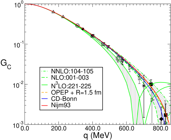
Figure 2: Results for the charge form factor $G_{C}$ as a function of $|{\bf q}|\equiv\sqrt{Q^{2}}$. The dashed lines show the largest and smallest form factors obtained with the NLO wave functions of Ref. [18]. The range of predictions with these wave functions is given by the horizontally shaded region. Similarly for the dot-dashed lines and the diagonally shaded region at NNLO, and the solid lines and the vertically shaded region at N³LO. Other results shown are for a wave function from Ref. [28] with $R=1.5$ fm (short-dashed line), and the Nijm93 and CD-Bonn deuteron wave functions (solid red and blue lines respectively). The experimental data is taken from the extraction of Ref. [53] and from Ref. [59]: upward triangles represent data from the $T_{20}$ measurement of Ref. [54], open circle [55], solid circle [56], open squares [57], downward triangles [58], rightward triangles [59], star [60], solid squares [61], solid diamonds [62].

It is worth noting that the NLO potential only includes $O(P^{2})$ corrections to $V$, and so the calculations labeled “NLO” in Fig. 2 are limited by the accuracy of the $NN$ potential. The calculations labeled “NNLO” have $O(P^{3})$ corrections included in the potential: the same level of accuracy to which the operator $J_{0}$ has been computed. In this respect only the computation with the NNLO wave functions is one that is carried out to a consistent order in both the wave functions and operators obtained using $\chi$ET. The results with the NLO and N³LO wave functions are shown for comparison. For the same reason we show results with the Nijm93 wave function, the CD-Bonn wave function, and the one-pion-exchange plus square well wave functions of Ref. [28]. In each case consistent choices for $\beta$ and $\nu$ (as explained in Sec. 3) were employed. In the case of all but the CD-Bonn and $\chi$ET N³LO calculations the impact of the $p^{2}/M^{2}$ pieces of the one-pion-exchange potential and the kinetic-energy operator has been assessed via the techniques described in Appendix A. Therefore all of these matrix elements have the same one-pion-exchange physics. A difference in their predictions is then either due to physics at the range of two-pion-exchange, or to physics at distances less than the scale where the chiral expansion can be used to reliably calculate the $NN$ potential.

In fact, Fig. 2 shows us that all of these wave functions predict very similar form factors for $|{\bf q}|\leq 600$ MeV. The most noticeable difference occurs around the zero of $G_{C}$—a region where, by definition, higher-order contributions cancel with lower-order contributions, and the calculation is therefore sensitive to the addition of higher-order effects. Most wave functions also produce a $G_{C}$ in good agreement with the data compilation of Abbott et al. [53] for $|{\bf q}|\leq 600$ MeV. An exception is the predictions using the N³LO wave function of Ref. [18], which diverge from those of the other wave functions considered here at significantly lower $Q^{2}$. Note also that the N³LO predictions seem to be significantly more sensitive to short-distance physics than is the case for the wave functions computed with NLO or NNLO chiral potentials, or even than the wave functions of Ref. [28], where only the result with the square well and surface delta function with $R=1.5$ fm is shown, but changing $R$ to 2.5 fm produces a barely discernible change in the short-dashed line.

It is possible that the situation with the predictions from the N³LO potential will improve when the pieces of $J_{0}$ of $O(eP^{4})$ and $O(eP^{5})$ which are not included in this calculation are added to the current operator. But, even if this is the case, sizeable cancellations between lower and higher-order effects are necessary if the N³LO wave function is to be used to describe electron-deuteron data at momentum transfers $Q^{2}\geq 0.2$ GeV².

One might argue that one does not expect the $\chi$ET to work beyond this scale anyway. However, the chiral expansion developed here and in Refs. [28, 32, 31] for the deuteron current operator still converges well at $Q^{2}\sim 0.3$ GeV². In part this is because the impulse (leading-order) result for $G_{C}$ can be written as:

$$G_{C}^{(0)}({\bf q})=\int_{0}^{\infty}\,d\hbox{r}\,j_{0}\left(\frac{|{\bf q}|r}{2}\right)(u^{2}(r)+w^{2}(r)),$$ (36)

where $j_{0}$ is a spherical Bessel function and $w(r)$ is the ³D₁ radial wave function. This means that—at least for the impulse-approximation piece of the matrix element—the relevant momentum scale at which the deuteron wave function is probed is not, in fact, $|{\bf q}|$, but $|{\bf q}|/2$—half of the momentum transfer is taken away by the center-of-mass degree of freedom. In this context the failure of the N³LO wave functions’ form-factor predictions to agree with the data when $|{\bf q}|/2\approx 200$ MeV is rather disturbing.

In Fig. 3 we show the results for $G_{Q}$. As mentioned above, the shape produced by all wave functions is remarkably similar—a point which was exploited in an extraction of $G_{E}^{(n)}$ in Ref. [66]. This can be understood from the presence of $j_{2}$, instead of the $j_{0}$ of Eq. (36) in the co-ordinate space integral that gives the leading-order contribution to $G_{Q}$. The pattern of convergence for $G_{Q}$ predictions with the order of the $\chi$ET potential is interesting. The NLO band is quite wide, and its centroid is below the data. The NNLO band is very narrow, and its centroid agrees well with data out to 800 MeV. We stress that this is the consistent order for computation of the potential, given the current operator we have used. The N³LO band is then as wide, and below, the NLO band. In this plot predictions using the Nijm93 and CD-Bonn potentials are not shown. But they lie within the diagonally-shaded band that represents the range of predictions of the NNLO $\chi$ET potential.

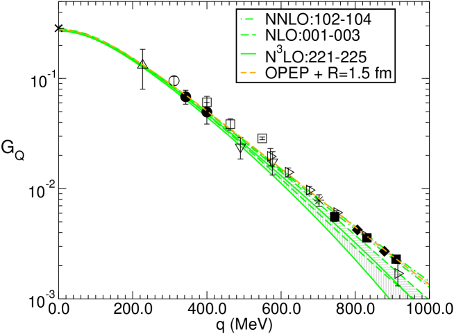
Figure 3: Results for the charge form factor $G_{Q}$ (in units of fm²) as a function of $|{\bf q}|\equiv\sqrt{Q^{2}}$. Legend as in Fig. 2, apart from the absence of curves for the Nijm93 and CD-Bonn wave functions. These curves fall within the range of the dot-dashed lines, i.e. the results with NNLO $\chi$ET wave functions.

	Experiment	NLO:001–003	NNLO:104–102	N3LO:221–225	Nijm93
$Q_{d}$ (fm2)	0.2859(3)	0.278–0.280	0.279–0.282	0.270–0.274	0.276

Table 2: Deuteron quadrupole moment computed with our NNLO charge operator and different wave functions. Results are accurate to the number of digits shown. The ranges are generated by considering various values of $\Lambda$ and $\bar{\Lambda}$ at a given order in the expansion for the $\chi$ET $NN$ potential. The “extremal” wave functions are indicated in the top line of the table.

In order to remove the rapid fall-off in the plots of Fig. 3 and 2, and also provide a result for the ratio of form factors which will be measured at BLAST at the momentum transfers indicated by the asterisks, we show predictions for the ratio $G_{C}/G_{Q}$ in Fig. 4. These predictions are compared to data from the compilation of Ref. [53], as well as the more recent data set from Novosibirsk [59] . As can easily be gleaned from Fig. 4, the different wave functions considered give predictions that disagree at about the 5% level at $Q^{2}=0$, i.e. they give different numbers for the deuteron quadrupole moment $Q_{d}$.

Numerical results for $Q_{d}$, computed with the NNLO operator that was used to generate the predictions of Fig. 4, are presented in Table 2. Note that the variation in the results with the $\chi$ET NLO and NNLO wave functions as the cutoffs $\Lambda$ and $\bar{\Lambda}$ are varied is of the same size as the discrepancy between those predictions and the experimental value (1).

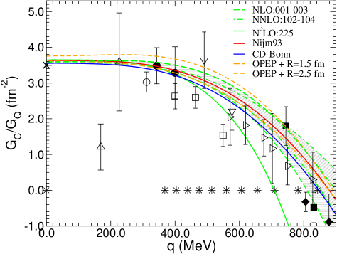
Figure 4: Results for the ratio $G_{C}/G_{Q}$. As in Fig. 2 the dashed lines and the horizontally shaded region show the range of results obtained with the NLO wave functions of Ref. [18]. Likewise for the dot-dashed lines and the diagonally shaded region at NNLO, and the solid lines and the vertically shaded region at N³LO. Other results shown are for wave functions from Ref. [28] with $R=1.5$ fm and $R=2.5$ fm (short-dashed lines), and the Nijm93 and CD-Bonn deuteron wave functions (solid red and blue lines respectively). Upward triangles are data from the $T_{20}$ measurement of Ref. [54], open circle [55], solid circle [56], open squares [57], downward triangles [58], rightward triangles [59], star [60], solid squares [61], solid diamonds [62]. The asterisks indicate the points where BLAST will extract this ratio from their $t_{20}$ data.

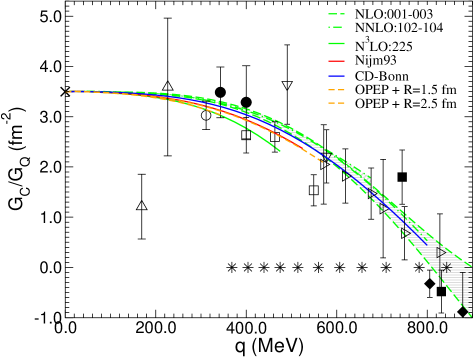
Figure 5: Results for $G_{C}/G_{Q}$, after $J_{0}^{(5)}$ is inserted with a coefficient adjusted to reproduce the experimental value of $Q_{d}$ and $\Lambda=1.5$ GeV. Legend as in Fig. 4. Each curve is shown only up to the point where the $J_{0}^{(5)}$ contribution is so large that the calculation is no longer reliable (with the exception of NLO).

The fact that short-distance physics can affect the value of $Q_{d}$ at the 2–3% level needed to restore agreement between theory and data encourages us to incorporate the operator $J_{0}^{(5)}$ (see Eq. (32)) in our calculation. In doing so we adopt the $Q^{2}$-dependence of Eq. (35) with $\Lambda=1500$ MeV. For each wave function the value of $h_{4}$ is adjusted to yield the experimental value of $Q_{d}$. The results of this procedure are presented in Fig. 5. The NNLO, N³LO, Nijm93, CD-Bonn, and one-pion-exchange-tail potential curves are only shown out to the momentum transfer where the contribution of the operator (32) makes up 20% of the contributions from the preceding orders. This gives a way to estimate where the calculations with various wave functions become unreliable: they are unreliable when $J_{0}^{(5)}$ is no longer a small piece of the total $G_{C}/G_{Q}$. Under this criterion most of the wave functions can give reliable predictions to $|{\bf q}|=500$–$600$ MeV, and below this value the wave-function dependence is markedly reduced as compared to what is seen in Fig. 4. Note that the lines at NLO are shown only to give an idea of the uncertainty coming from sensitivity to the choice of $(\Lambda,\bar{\Lambda})$. Their predictions with this wave function for $G_{C}/G_{Q}$ beyond 600 MeV are provided only for recreational purposes.

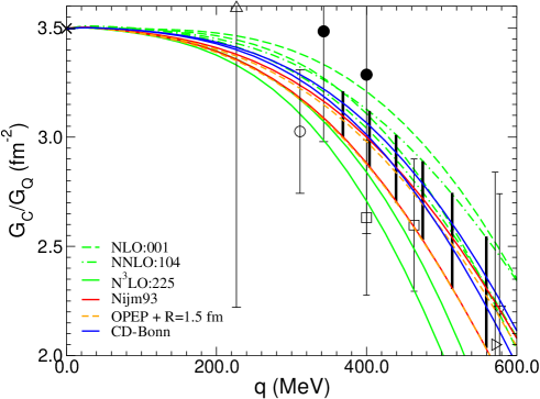
Figure 6: Results for $G_{C}/G_{Q}$, showing the variation that results from ignorance of the $Q^{2}$-dependence of the operator $J_{0}^{(5)}$ ($\Lambda=1.2$–$2$ GeV). Calculations are shown for NLO (long dashed), NNLO (dot-dashed), N³LO (solid green), Nijm93 (solid red), CD-Bonn (solid blue) and $R=1.5$ fm square well + one-pion exchange (short dashed) wave functions. The vertical lines indicate a reasonable range for the theoretical prediction at each of the points where BLAST will have data. The experimental data is from Refs. [54] (upward triangle), [55] (open circle), [56] (solid circle), and [57] (open square). Note change of scale as compared to Fig. 5.

$|{\bf q}|$ (MeV)	$G_{C}/G_{Q}$ (fm2)	Error bar (fm2)
368.4	3.11	0.11
403.9	2.99	0.13
439.3	2.86	0.16
474.8	2.71	0.18
514.2	2.53	0.22
559.5	2.29	0.26
606.8	2.02	0.30

Table 3: Predictions for the ratio $G_{C}/G_{Q}$ at the values of $|{\bf q}|$ where this quantity will be measured at BLAST. The error bar and central values displayed here are obtained via the procedure discussed in the text.

Lastly we focus on the region where the $\chi$ET is reliable: $|{\bf q}|\leq 600$ MeV. An enhanced view of this region is shown in Fig. 6. For each choice of $NN$ potential two curves are shown: the upper one of the pair corresponds to choosing $\Lambda=1.2$ GeV when evaluating the operator $J_{0}^{(5)}$ and the lower one corresponds to choosing $\Lambda=2$ GeV. A conservative estimate for the impact of short-distance physics which is not well-constrained in this $\chi$ET calculation is given by combining the uncertainties from $(\Lambda,\bar{\Lambda})$ variation and the uncertainty coming from lack of knowledge about the momentum dependence of $J_{0}^{(5)}$. The black bars then represent the range of possible values that the $\chi$ET predicts for $G_{C}/G_{Q}$ at the kinematics where there will be data from BLAST. These ranges are reproduced in Table 3. The error is about $\pm 3$% at the lowest BLAST point and increases with $Q^{2}$, as it should. Note that we have not included the N³LO $\chi$ET wave function, or the NLO $\chi$ET wave function, in generating these predictions. As already discussed, the predictions for $G_{C}$ and $G_{Q}$ with the N³LO wave function deviate already from the extant data at quite low $Q^{2}$, while the NLO wave function is, in the $\chi$ET sense, less accurate than the operator being used here. The predictions obtained with these wave functions are, however, within 2$\sigma$, if the theoretical error bars we have obtained are taken to have the usual one-standard-deviation interpretation.

6 Results for $G_{C}/G_{M}$

BLAST will also measure the ratio $G_{C}/G_{M}$. Predictions for that observable are provided in Fig. 7. We do not show any experimental data in Fig. 7 because, as far as we can glean from the literature, all previous data on $G_{M}$ comes from different data sets to that used for the extraction of $G_{Q}$ and $G_{C}$ [53]. Therefore in general data on $G_{C}$ and $G_{M}$ are not at the same $Q^{2}$ and have different systematic errors. The BLAST data set will be pioneering in this regard.

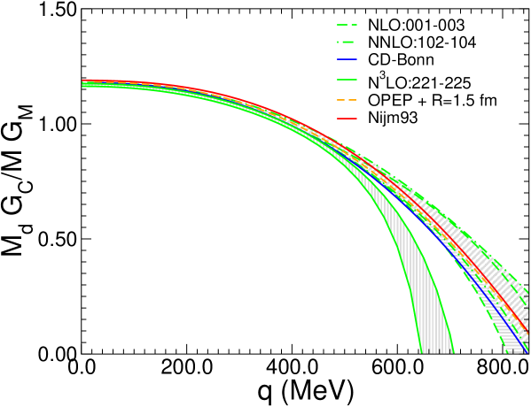
Figure 7: Results for the ratio $G_{C}/G_{M}$. Calculations shown are for extremal NLO (long dashed), extremal NNLO (dot-dashed), extremal N³LO (solid green) (solid red), CD-Bonn (solid blue) and $R=1.5$ fm square well + one-pion exchange (short dashed) wave functions.

The calculations displayed in Fig. 7 are accurate to relative order $P^{2}$, although the $G_{C}$ used here is actually computed up to relative order $P^{3}$. Once again the shape of the low-momentum part of the ratio is fairly wave-function independent, but the value at $Q^{2}=0$ changes as we move through the different wave functions used for the computation of Fig. 7, due to short-distance contributions to $\mu_{d}$ being different for different wave functions. However, even without renormalization there is a robust prediction for the ratio out to $Q^{2}\approx 0.1$ GeV². The robust prediction is that $G_{C}/G_{M}$ is approximately flat. This would be exactly the case in the absence of relativistic, meson-exchange, and nucleon-structure contributions to the operator, and if $w(r)=0$. The relativistic corrections at $O(P^{2})$ are negligible at $Q^{2}<0.1$ GeV², and the meson-exchange piece of the charge operator is higher order than we are attempting to calculate the ratio $G_{C}/G_{M}$ to. As far as the operator is concerned this leaves only the nucleon-structure effects, which depend on the ratio:

$$\frac{G_{E}^{(s)}}{G_{M}^{(s)}}.$$ (37)

If a strict chiral expansion is used for the form factors then this ratio depends (again, at this order) on the difference of the isoscalar magnetic and charge radii, and amounts to a $<10$% effect at $Q^{2}=0.1$ GeV². Even though taking the ratio $G_{C}/G_{M}$ does not (as it did in the case of the ratio of the previous section) eliminate nucleon-structure effects, it does reduce their size. Meanwhile, the effects of $w$ grow with $Q^{2}$, and so at $Q^{2}<0.1$ GeV² it is thus not particularly surprising that $G_{M}/G_{C}$ is, to quite a good approximation, flat.

Given the extent of the variation in the prediction for the ratio beyond $|{\bf q}|=500$ MeV it is difficult to believe that the NLO predictions for the ratio shown here are reliable beyond that point. This situation could improve once the NNLO pieces of the operator ${\bf J}$ were computed, but short-distance pieces of ${\bf J}$ appear already at that order. Therefore it is a prediction of the chiral expansion that this ratio will be more sensitive to short-distance physics than is $G_{C}/G_{Q}$. The position of the minimum in $G_{M}$ is known to be very sensitive to such short-distance physics [47, 63, 64, 65]. In this context it is worth noting that the minimum for the N³LO wave functions is already at $|{\bf q}|\approx 800$ MeV—much lower than in any of the calculations of Refs. [47, 63, 64, 65] and indeed, much lower than the experimental data allows the position of the minimum to be [53].

7 Conclusion

We have used the $\chi$ET isoscalar charge operator in the nucleon-nucleon sector computed to NNLO (including a consistent treatment of the $1/M$ pieces of the charge), and the wave functions of Ref. [18], to obtain the form-factor ratios $G_{C}/G_{E}^{(s)}$, $G_{Q}/G_{E}^{(s)}$, $G_{C}/G_{Q}$. These ratios test $\chi$ET’s ability to describe deuteron structure. We confirm and extend the finding of Ref. [31], that the NLO and NNLO $\chi$ET wave functions, combined with the NNLO $J_{0}$, yield results for these ratios that agree—within the experimental uncertainties—with the extractions of Ref. [53] for $Q^{2}<0.35$ GeV². In contrast, the N³LO wave function of Ref. [18], when used in conjunction with the N²LO charge operator, produces form factors that depart from the data at $Q^{2}\approx 0.2$ GeV².

In light of the upcoming release of data on $t_{20}$ from BLAST we examined the ratio $G_{C}/G_{Q}$ in detail. We found variation in the $\chi$ET predictions for this ratio at $Q^{2}=0$, and also found that—even allowing for this variation—$\chi$ET is in disagreement with the experimental value for this quantity. This phenomenon—the “$Q_{d}$ problem”—is familiar in high-precision $NN$ potential models with the modern value of the $\pi$NN coupling constant. In $\chi$ET its solution arises naturally through a higher-order two-body current that couples exclusively to quadrupole photons. We added this operator to our analysis, and showed that when we do so the $\chi$ET predictions for $G_{C}/G_{Q}$ (with the NNLO wave functions) fall within a narrow band out to $Q^{2}\approx 0.35$ GeV² (see Fig. 6). We also performed the calculation with the same charge operator and potential-model wave functions that have a one-pion-exchange tail identical to that of the $\chi$ET potential [26, 27, 28]. We found that these wave functions make the band obtained at NNLO in $\chi$ET about a factor of two wider. We conservatively adopt the full width of that band as representative of the theoretical uncertainty in our calculation.

Meanwhile, the $\chi$ET predictions for $G_{C}/G_{M}$, which will also be measured at BLAST, are not reliable to as high a $Q^{2}$. In saying this, it should, in fairness, be pointed out that ${\bf J}$ has not been computed to as high an order as $J_{0}$, and it could therefore be that $G_{C}/G_{M}$ can also be well described to $Q^{2}=0.35$ GeV² in $\chi$ET once $O(eP^{4})$ corrections to $\bf J$ are included. This is a topic for future work. Another topic for future work is the inclusion of the $O(eP^{4})$ pieces of $J_{0}$ that were already computed in Ref. [40] at $Q^{2}=0$ in the finite-$|{\bf q}|$ calculation [46]. In addition, the operators and the $\chi$ET wave functions used in this paper to make predictions for the BLAST data can be further tested by comparing their predictions with experimental results for deuteron electro-disintegration—although this will require the computation of the isovector pieces of the operators.

Irrespective of such future efforts, one thing is already clear from Fig. 6. When the theoretical predictions for $G_{C}/G_{Q}$ are renormalized in the manner we advocate here, the theoretical uncertainty in $G_{C}/G_{Q}$ for $Q^{2}\leq 0.3$ GeV² is less than the uncertainty in the data. This makes the low-$Q^{2}$ data from BLAST all the more crucial, since it will provide an important test of $\chi$ET’s ability to organize contributions to deuteron observables, and its ability to use that organization to provide estimates of the theoretical uncertainty in a given calculation.

Appendix A Including $p^{2}/M^{2}$ corrections in “non-relativistic” wave functions

One way to include relativistic corrections to the nucleon kinetic energy operator in the $\chi$ET is to solve the “relativistic Schrödinger equation” [18]

$$2\left[\sqrt{p^{2}+M^{2}}-M\right]\psi_{l}^{sj}(p)+\int\frac{dp^{\prime}{p^{\prime}}^{2}}{(2\pi)^{3}}\,V_{ll^{\prime}}^{sj}(p,p^{\prime})\psi_{l^{\prime}}^{sj}(p^{\prime})=E\psi_{l}^{sj}(p),$$ (38)

with the (partial-wave decomposed) potential $V_{ll^{\prime}}^{sj}(p,p^{\prime})$ the one that is obtained from the $\chi$ET using the counting rules explained in Section 1. To facilitate computation of the $p^{2}/M^{2}$ (and beyond) corrections to the nucleon kinetic energy operator we adopt the Kamada-Glöckle transformation [45] and define a new relative momentum $\tilde{p}$ such that

$$\frac{\tilde{p}^{2}}{2M}=\sqrt{M^{2}+p^{2}}-M.$$ (39)

The inverse transformation is then:

$$p=\tilde{p}\sqrt{1+\frac{\tilde{p}^{2}}{4M^{2}}}\equiv\tilde{p}g(\tilde{p}).$$ (40)

As shown by Kamada and Glöckle, any “relativistic” Schrödinger equation that employs the kinetic energy operator with the relativistic form on the right-hand side of Eq. (39) can be recast as a non-relativistic Schrödinger equation, i.e. [45, 18]

$$\frac{\tilde{p}^{2}}{2M}\tilde{\psi}_{l}^{sj}(\tilde{p})+\int\frac{d\tilde{p}^{\prime}\tilde{p}^{\prime\,2}}{(2\pi)^{3}}\,\,\tilde{V}_{ll^{\prime}}^{sj}(\tilde{p},\tilde{p}^{\prime})\tilde{\psi}_{l^{\prime}}^{sj}(\tilde{p}^{\prime})=E\tilde{\psi}_{l}^{sj}(\tilde{p}),$$ (41)

where the potential $\tilde{V}_{ll^{\prime}}^{sj}$ is obtained from $V_{ll^{\prime}}^{sj}$ via:

$$\tilde{V}_{ll^{\prime}}^{sj}(\tilde{p},\tilde{p}^{\prime})=h(\tilde{p})V_{ll^{\prime}}^{sj}(\tilde{p}g(\tilde{p}),\tilde{p}^{\prime}g(\tilde{p}^{\prime}))h(\tilde{p}^{\prime}),$$ (42)

and

$$\tilde{\psi}(\tilde{p})=h(\tilde{p})\psi(\tilde{p}g(\tilde{p})).$$ (43)

Here the factor $h$ is introduced to ensure that, as long as $\psi$ is normalized to one, $\tilde{\psi}$ is also normalized to one. Calculation of the Jacobian associated with the transformation (39) yields:

$$h(\tilde{p})=\sqrt{\left(1+\frac{\tilde{p}^{2}}{2M^{2}}\right)g(\tilde{p})}.$$ (44)

We can also work this procedure in reverse, i.e. interpret solutions of the non-relativistic Schrödinger equation as solutions to a dynamical equation with a relativistic kinetic energy operator and a relativistic potential. (Something similar is done to obtain the $NN$ c.m. frame Hamiltonian in approaches to electron-deuteron scattering based on Relativistic Hamiltonian Dynamics, see, for example, Ref. [67].). Here we will make this interpretation for the deuteron wave functions obtained with the NLO and NNLO chiral potentials.

Suppose that $\tilde{V}$ is the chiral potential computed (at NLO or NNLO) without $p^{2}/M^{2}$ corrections, i.e.

$$\tilde{V}_{ll^{\prime}}^{sj}(\tilde{p},\tilde{p^{\prime}})=f(\tilde{p}){\cal M}_{ll^{\prime}}^{sj}(\tilde{p},\tilde{p}^{\prime})f(\tilde{p}^{\prime}),$$ (45)

where ${\cal M}$ is the (partial-wave decomposed) sum of $NN$-irreducible diagrams that is computed at NLO and NNLO using spectral-function regularization in Ref. [18] and $f(p)=\exp(-p^{6}/\Lambda^{6})$ is the “Lippmann-Schwinger equation regulator” used there. A potential $V$ that includes $p^{2}/M^{2}$ corrections and is associated with the same sum of Feynman diagrams can be constructed by inverting Eq. (42). We find that this potential, which when inserted in the relativistic Schrödinger equation (38) will be phase-equivalent to $\tilde{V}$ of Eq. (45), is:

$$V_{ll^{\prime}}^{sj}(p,p^{\prime})=\frac{f(p)}{h(p)}{\cal M}_{ll^{\prime}}^{sj}\left(\sqrt{2M\sqrt{M^{2}+p^{2}}-2M^{2}},\sqrt{2M\sqrt{M^{2}+p^{\prime 2}}-2M^{2}}\right)\frac{f(p^{\prime})}{h(p^{\prime})}.$$ (46)

We have not bothered to distinguish between $\tilde{p}$ and $p$ in the functions $f$ and $h$, because we now define a new regulator function $\overline{f}\equiv f/h$ to obtain:

$$V_{ll^{\prime}}^{sj}(p,p^{\prime})=\overline{f}(p){\cal M}_{ll^{\prime}}^{sj}\left(\sqrt{2M\sqrt{M^{2}+p^{2}}-2M^{2}},\sqrt{2M\sqrt{M^{2}+p^{\prime 2}}-2M^{2}}\right)\overline{f}(p^{\prime}),$$ (47)

up to terms that are of order $p^{4}/M^{4}$. Since we count $M$ as the same order as the cutoff scale $\Lambda$ absorbing the functions $h$ into the definition of the regulator in this way makes physical sense. Apart from these short-distance effects the only difference between the potentials $V$ and $\tilde{V}$ is the use of the “stretched” momenta in $V$.

If we wish we can also incorporate the factor $\left(1-\frac{p^{2}+p^{\prime 2}}{2M^{2}}\right)$ that distinguishes Eq. (26) from the non-relativistic treatment of one-pion exchange used at NLO and NNLO in Ref. [18]. To do this we redefine the regulator again, writing

$$V_{ll^{\prime}}^{sj}(p,p^{\prime})=\overline{\overline{f}}(p)\left(1-\frac{p^{2}}{2M^{2}}\right){\cal M}_{ll^{\prime}}^{sj}\left(\sqrt{2M\sqrt{M^{2}+p^{2}}-2M^{2}},\sqrt{2M\sqrt{M^{2}+p^{\prime 2}}-2M^{2}}\right)$$

$$\left(1-\frac{p^{\prime 2}}{2M^{2}}\right)\overline{\overline{f}}(p^{\prime}),$$ (48)

where, up to the order to which we work:

$$\overline{\overline{f}}(p)=\left(1+\frac{3p^{2}}{16M^{2}}\right)\exp\left(-\frac{p^{6}}{\Lambda^{6}}\right).$$ (49)

If one ignores the regulator $\overline{\overline{f}}$, then the factors in front of the one-pion-exchange part of the potential in Eq. (48) agree with Eq. (26) and the expression for the two-pion-exchange pieces has been modified only at N³LO and beyond. As for the short-distance pieces of the potential, the changes in the way the chiral $NN$ potential is regularized ($f\rightarrow\overline{f}\rightarrow\overline{\overline{f}}$) mean that the $NN$ LEC $C_{2}$ will have to be re-defined: its value is shifted by a term of $O(1/M^{2})$. However, $C_{2}$ is fitted to data, so no change in observables should result from doing this.

Therefore we have shown that, via modifications of the (unobservable) short-distance part of the potential that do not affect the low-energy observables, we can absorb much of the “relativistic effects” that would enter the NLO and NNLO chiral potentials were we to count $M\sim\Lambda$. The only such effect that cannot be absorbed by a redefinition of the regulator used when solving the Lippmann-Schwinger equation with the potential $V$ is the different arguments at which ${\cal M}$ is evaluated in Eq. (48) as compared to Eq. (45). This difference is an NLO effect for the part of $V$ coming from one-pion exchange, where it represents the interplay of the relativistic kinetic energy operator and the (leading-order) one-pion-exchange potential. This interplay is not included in our calculations, but all other relativistic effects are, and as reported in Sec. 3, they prove to be small.

The main difference between interpreting the expression (45) as a non-relativistic potential and interpreting it as resulting from a relativistic calculation after application of the Kamada-Glöckle transformation therefore resides in the momentum arguments that enter the Schrödinger equation. In the first case the wave function that is the solution of that equation will be a function of $\tilde{p}$. In the second case it will be a function of $p=\sqrt{2M\sqrt{M^{2}+\tilde{p}^{2}}-2M^{2}}$. The relationship between the two wave functions is given by Eq. (43). This can be inverted to yield Eq. (30), which we rewrite here:

$$\psi(p)=\sqrt{\frac{M}{\sqrt{M^{2}+p^{2}}}}\left(\frac{2M}{M+\sqrt{M^{2}+p^{2}}}\right)^{1/4}\tilde{\psi}\left(\sqrt{2M\sqrt{M^{2}+p^{2}}-2M^{2}}\right).$$ (50)

Thus, if we are provided with the wave-function $\tilde{\psi}$ that is obtained by solving the non-relativistic Schrödinger equation with the potential $\tilde{V}$, then we may derive from that the wave function $\psi$, that is the solution of the relativistic Schrödinger equation (38) with a phase-equivalent relativistic potential $V$ (48), with $V$ constructed to include all the corrections to one-pion-exchange that must be present in the NLO and NNLO potentials if we count $M\sim\Lambda$. This procedure is not necessary in the case of the N³LO potential. In that case the $1/M^{2}$ corrections which are connected with the current (27) were explicitly computed in Ref. [18].

References

- [1] R. F. Code and N. F. Ramsey, Phys. Rev. A 4, 1945 (1971).
- [2] D. M. Bishop and L. M. Cheung, Phys. Rev. C 20, 381 (1979).
- [3] P. J. Mohr and B. N. Taylor, Rev. Mod. Phys. 72, 351 (2000).
- [4] R. Gilman and F. Gross, J. Phys. G 28, R37 (2002).
- [5] M. Garcon and J. W. Van Orden, Adv. Nucl. Phys, 26, 293 (2001).
- [6] I. Sick, Prog. Part. Nucl. Phys. 47, 245 (2001).
- [7] S. R. Beane et al., in At the frontier of particle physics, vol. 1, edited by M. Shifman (World Scientific, Singapore, 2000).
- [8] P. F. Bedaque and U. van Kolck, Ann. Rev. Nucl. Part. Sci. 52, 339 (2002).
- [9] D. R. Phillips, J. Phys. G 31, S1263 (2005), and references therein.
- [10] E. Epelbaum, Prog. Part. Nucl. Phys. 57, 654 (2006).
- [11] S. Weinberg, Phys. Lett. B. 251, 288 (1990).
- [12] S. Weinberg, Nucl. Phys. B363, 3 (1991).
- [13] S. Weinberg, Phys. Lett. B. 295, 114 (1992).
- [14] C. Ordóñez and U. van Kolck, Phys. Lett. B 291, 459 (1992); C. Ordóñez, L. Ray, and U. van Kolck, Phys. Rev. C 53, 2086 (1996).
- [15] E. Epelbaum, W. Glöckle, and U.-G. Meißner, Nucl. Phys. A671, 295 (2000).
- [16] D. R. Entem and R. Machleidt, Phys. Lett. B524, 93 (2002).
- [17] D. R. Entem and R. Machleidt, Phys. Rev. C 68, 041001 (2003).
- [18] E. Epelbaum, W. Glöckle, and U.-G. Meißner, Nucl. Phys. A 747, 362 (2005);
- [19] E. Epelbaum, W. Glöckle and U. G. Meissner, Eur. Phys. J. A 19, 125 (2004); ibid., 401.
- [20] D. B. Kaplan, M. J. Savage and M. B. Wise, Nucl. Phys. B 478, 629 (1996).
- [21] S. R. Beane, P. F. Bedaque, M. J. Savage and U. van Kolck, Nucl. Phys. A 700, 377 (2002).
- [22] D. Eiras and J. Soto, Eur. Phys. J. A 17, 89 (2003).
- [23] A. Nogga, R. G. E. Timmermans and U. van Kolck, Phys. Rev. C 72, 054006 (2005).
- [24] M. Pavon Valderrama and E. Ruiz Arriola, Phys. Rev. C 72, 054002 (2005).
- [25] M. C. Birse, Phys. Rev. C 74, 014003 (2006).
- [26] V. G. J. Stoks, R. A. M. Klomp, C. P. F. Terheggen and J. J. de Swart, Phys. Rev. C 49, 2950 (1994).
- [27] R. Machleidt, Phys. Rev. C 63, 024001 (2001).
- [28] D. R. Phillips and T. D. Cohen, Nucl. Phys. A668, 45 (2000).
- [29] J.-W. Chen, G. Rupak, and M. Savage, Nucl. Phys. A653, 386 (1999).
- [30] V. Bernard, N. Kaiser, and U.-G. Meißner, Int. Jour. of Mod. Phys. E 4, 193 (1995).
- [31] D. R. Phillips, Phys. Lett. B 567, 12 (2003).
- [32] M. Walzl and U. G. Meißner, Phys. Lett. B513, 37 (2001).
- [33] J. Adam and H. Arenhövel, Nucl. Phys. A614, 289 (1997).
- [34] D. O. Riska, Prog. Part. Nucl. Phys. 11, 199 (1984).
- [35] V. Bernard, H. W. Fearing, T. R. Hemmert and U. G. Meißner, Nucl. Phys. A 635, 121 (1998) [Erratum-ibid. A 642, 563 (1998)].
- [36] S. Platchkov et al., Nucl. Phys. A 510, 740 (1990).
- [37] P. Mergell, U. G. Meißner and D. Drechsel, Nucl. Phys. A 596, 367 (1996).
- [38] T.-S. Park, D.-P. Min, and M. Rho, Nucl. Phys. A596, 515 (1996).
- [39] M. J. Savage, K. A. Scaldeferri, and M. B. Wise, Nucl. Phys. A652, 273 (1999).
- [40] T.-S. Park, K. Kubodera, D.-P. Min, and M. Rho, Phys. Lett. B472, 232 (2000).
- [41] J. Adam, H. Goller, and H. Arenhövel, Phys. Rev. C 48, 470 (1993).
- [42] J. L. Friar, Phys. Rev. C 22, 796 (1980).
- [43] J. L. Forest, Phys. Rev. C 61, 034007 (2000).
- [44] E. Epelbaum, W. Glöckle and U. G. Meißner, Nucl. Phys. A 637, 107 (1998).
- [45] H. Kamada and W. Glöckle, Phys. Rev. Lett. 80, 2547 (1998).
- [46] Y.-H. Sung, T.-S. Park, N. Kaiser, and D. R. Phillips, in progress.
- [47] R. B. Wiringa, V. G. J. Stoks, and R. Schiavilla, Phys. Rev. C 51, 38 (1995).
- [48] E. Epelbaum, U. G. Meissner, W. Gloeckle and C. Elster, Phys. Rev. C 65, 044001 (2002).
- [49] E. Truhlik, J. Smejkal and F. C. Khanna, Nucl. Phys. A 689, 741 (2001).
- [50] J. J. de Swart, C. P. F. Terheggen and V. G. J. Stoks, arXiv:nucl-th/9509032.
- [51] W. P. Sitarski, P. G. Blunden and E. L. Lomon, Phys. Rev. C 36, 2479 (1987); P. G. Blunden, W. R. Greenberg and E. L. Lomon, Phys. Rev. C 40, 1541 (1989).
- [52] A. Amghar, N. Aissat and B. Desplanques, Eur. Phys. J. A 1, 85 (1998).
- [53] D. Abbott et al., Eur. Phys. J. A7, 421 (2000).
- [54] V. F. Dmitriev et al., Phys. Lett. B. 157, 143 (1985).
- [55] M. Ferro-Luzzi et al., Phys. Rev. Lett. 77, 2630 (1996).
- [56] M. E. Schulze et al., Phys. Rev. Lett. 52, 597 (1984).
- [57] M. Bouwhuis et al., Phys. Rev. Lett. 82, 3755 (1999).
- [58] R. Gilman et al., Phys. Rev. Lett. 65, 1733 (1990).
- [59] D. M. Nikolenko et al., Phys. Rev. Lett. 90, 072501 (2003).
- [60] B. Boden et al. Z. Phys. C49, 175 (1991).
- [61] M. Garcon et al., Phys. Rev. C49, 2516 (1994).
- [62] D. Abbott et al., Phys. Rev. Lett. 84, 5053 (2000).
- [63] J. W. Van Orden, N. Devine and F. Gross, Phys. Rev. Lett. 75, 4369 (1995).
- [64] R. Schiavilla and V. R. Pandharipande, Phys. Rev. C65, 064009 (2002).
- [65] D. R. Phillips, S. J. Wallace and N. K. Devine, Phys. Rev. C 72, 014006 (2005).
- [66] R. Schiavilla and I. Sick, Phys. Rev. C 64, 041002 (2001).
- [67] P. L. Chung, W. N. Polyzou, F. Coester and B. D. Keister, Phys. Rev. C 37, 2000 (1988).