On the convergence of multi-channel effective interactions

Abstract

A detailed analysis of convergence properties of the Andreozzi-Lee-Suzuki iteration method, which is used for the calculation of low-momentum effective potentials $V_{\text{low }k}$ is presented. After summarizing different modifications of the iteration method for one-flavor channel we introduce a simple model in order to study the generalization of the iteration method to multi-flavor channels. The failure of a straightforward generalization is discussed. The introduction of a channel-dependent cutoff cures the conceptual and technical problems. This novel method has already been applied successfully for realistic hyperon-nucleon interactions.

I Introduction

In Ref. Bogner et al. (2003) Bogner et al. have developed a low-momentum $NN$ interaction $V_{\text{low }k}$ which is constructed by a combination of renormalization group (RG) ideas and effective field theory approaches. Starting from a realistic nucleon-nucleon interaction in momentum space for the two-nucleon system, the $V_{\text{low }k}$ is obtained by integrating out the high-momentum components of the potential. In this way a cutoff momentum $\Lambda$ is introduced to specify the boundary between the low- and high-momentum space. Since the physical low-energy quantities such as phase shifts or the deuteron binding energy must not depend on the cutoff, the full-on-shell $T$-matrix has to be preserved for the relative momenta $k,k^{\prime}<\Lambda$. This yields an exact RG flow equation for a cutoff-dependent effective potential $V_{\text{low }k}$, which is based on a modified Lippmann-Schwinger equation (LSE).

Instead of solving the RG flow equation, which is a differential equation, with standard methods (e.g. Runge-Kutta method) directly, an iteration method is used. This iteration method, pioneered by Andreozzi, Lee and Suzuki (ALS) Lee and Suzuki (1980a); Suzuki and Lee (1980); Andreozzi (1996), is based on a similarity transformation and its solution corresponds to solving the flow equation Bogner et al. (2001).This transformation is also used for the effective interaction in the no-core shell model (e.g. Navratil et al. (2000); Stetcu et al. (2005)).

In Ref. Schaefer et al. (2006) the $V_{\text{low }k}$ approach was generalized to the hyperon-nucleon ($YN$) interaction with strangeness $S=-1$. For hyperons with strangeness $S=-1$, two isospin states $I=1/2$ and $I=3/2$ are available. For $I=1/2$, several coupled hyperon-nucleon channels occur that require new technical developments in the iteration method as already outlined in Ref. Schaefer et al. (2006). Especially, the $\Lambda N\leftrightarrow\Sigma N$ transition involves a mass difference of $\approx 78\,\text{MeV}$ and causes the failure of the known methods. In the present study we discuss these novel technical modifications in detail and investigate the convergence of the ALS iteration methods.

The paper is organized as follows: In the next Sec. we summarize the ALS iteration method for the one-flavor channel and discuss several modifications which improve its convergence. The generalization of the ALS method to multi-flavor channels is presented in the following Section. Instead of working with a realistic hyperon-nucleon interaction we introduce a simple solvable model in order to elucidate the essential modifications of the iteration method. We end with a summary and outlook.

II One-flavor Channel

The so-called model space (or $P$-space) is introduced in order to truncate the infinitely many degrees of freedom of a Hilbert space to a finite, low-energy subspace. The projection operator $P$ onto the model space and its complement projection operator $Q$ onto the excluded space are defined by

$$P\equiv\sum\limits_{i=1}^{d}\left|{\phi_{i}}\right\rangle\!\left\langle{\phi_{i}}\right|\quad\ ;\qquad Q=1-P\ ,$$ (1)

where $d$ denotes the dimension of the model space. The wave functions $\left|{\phi_{i}}\right\rangle$ are eigenfunctions of the unperturbed Hamiltonian $H_{0}$, which is composed of the kinetic energy and an arbitrary one-body potential.

Employing this separation of the Hilbert space, the original full Hamiltonian $H$ can then be replaced by a transformed Hamiltonian $\mathcal{H}$ that acts only on the low-energy model subspace. In particular, if $\left|{\Psi_{i}}\right\rangle$ is an eigenstate of the full Hamiltonian $H$ then its projection onto the model space $\left|{\psi^{M}_{i}}\right\rangle=P\left|{\Psi_{i}}\right\rangle$ satisfies the Schrödinger equation

$$\mathcal{H}\left|{\psi^{M}_{i}}\right\rangle=E_{i}\left|{\psi^{M}_{i}}\right\rangle\ .$$ (2)

The crucial point is that the eigenvalues $E_{i}$ of the transformed Hamiltonian are the same as those of the original Hamiltonian.

On the other hand, the transformation of all model states $\left|{\psi^{M}_{i}}\right\rangle$ back into the exact states defines a non-singular wave operator $\Omega$ via $\left|{\Psi_{i}}\right\rangle=\Omega\left|{\psi^{M}_{i}}\right\rangle$. Assuming that this wave operator has an inverse, the transformed Hamiltonian is related to the full Hamiltonian by a similarity transformation

$$\mathcal{H}=\Omega^{-1}H\Omega\ .$$ (3)

There is no unique representation for the wave operator $\Omega$. Different choices for $\Omega$ may then give different results for the perturbative expansion of the transformed interaction. Furthermore, even the same defining equation for $\Omega$ can be solved by different iterative schemes. As an example one often employs the ansatz by Lee and Suzuki Lee and Suzuki (1980a); Suzuki and Lee (1980) for the wave operator

$$\Omega=e^{\omega}$$ (4)

where $\omega$ is known as the correlation operator. The correlation operator generates the component of the wave function in the $Q$-space and can be expanded in terms of Feynmann–Goldstone diagrams Hjorth-Jensen et al. (1995). One choice for the correlation operator is

$$\omega=Q\mathcal{\omega}P$$ (5)

and thus we have $\Omega=1+\omega$.

Applying the operator $Q$ on Eq. (2), one immediately obtains $Q\mathcal{H}P=0$. Together with Eq. (3), this then leads to the so-called decoupling equation

$$\omega PHQ\omega+\omega PHP-QHQ\omega-QHP=0$$ (6)

which is to be solved in $\omega$ by iteration. For this non-linear matrix equation no general solution method is known, nor the number of existing solutions.

In this work we will discuss and generalize the solution of the decoupling equation for arbitrary coupled channels. The construction of the solution is based on the iteration method after Lee and Suzuki Lee and Suzuki (1980a, b) and Andreozzi Andreozzi (1996), labeled as ’ALS iteration’ in the following.

II.1 The ALS iteration

We start with an overview of the main ingredients of the standard ALS iteration. As already mentioned, this is not the only existing method which solves the decoupling equation.

Defining the model space effective Hamiltonian,

$$p\left(\omega\right)=P\mathcal{H}P=PHP+PHQ\omega\ ,$$ (7)

and its complement $Q$-space Hamiltonian,

$$q\left(\omega\right)=Q\mathcal{H}Q=QHQ-\omega PHQ\ ,$$ (8)

an iterative solution $\omega_{sol}\equiv\sigma$ of Eq. (6) can be obtained by

$$\sigma=\sum_{n=0}^{\infty}x_{n}\ ,$$ (9)

where the ${x_{n}}$’s satisfy successively

$$x_{0}=\frac{-1}{QHQ}QHP\ ,$$

$$x_{1}=\frac{1}{q\left(x_{0}\right)}x_{0}p\left(x_{0}\right)\ ,$$

$$\vdots$$

$$x_{n}=\frac{1}{q\left(x_{0}+\cdots+x_{n-1}\right)}x_{n-1}p\left(x_{0}+\cdots+x_{n-1}\right)\ .$$

Once a solution of these equations is known, the low-momentum effective Hamiltonian can be expressed as

$$\mathcal{H}_{\text{low }k}=p(\sigma)\ .$$ (10)

Subtracting from $\mathcal{H}_{\text{low }k}$ the kinetic energy in the model space, $PH_{0}P$, this yields the wanted low-momentum potential $V_{\text{low }k}$. As a remark we note, that this iterative solution $\sigma$ is equivalent to the LS vertex renormalization solution (see Refs. Lee and Suzuki (1980b, a)).

Since $x_{n}\to 0$ for large $n$, only a finite number of terms in the sum (9) are needed numerically in order to reach a desired precision. Furthermore, this condition implies for each iteration step $n$ the relation

$$\left|\lambda_{pM}\right|<\left|\lambda_{qm}\right|\ ,$$ (11)

where $\lambda_{pM}$ is the largest $P$-space eigenvalue (absolute value) and $\lambda_{qm}$ the smallest $Q$-space eigenvalue. Thus, as a necessary condition, this iteration method converges to the $d$ eigenvalues of the Hamiltonian of smallest absolute value.

A slight variation of the standard ALS iteration consists in the subtraction of a constant multiple of the identity, $m_{0}I$, from the full Hamiltonian $H$. In this case the iteration will converge to the shifted set of $d$ eigenvalues which are nearest to the chosen constant $m_{0}$. The choice of $m_{0}$ is not arbitrary. One has to make sure that the eigenvalues closest to $m_{0}$ are really inside the $P$-space. For numerical applications, this variation can also be used to accelerate the iteration since the required shift of the eigenvalues is smaller if $m_{0}$ is included. Furthermore, calculating the $V_{\text{low }k}$ for the hyperon-nucleon Nijmegen potential  Rijken et al. (1999) (cf. Ref. Schaefer et al. (2006)) the constant shift in the iteration is useful to avoid an unphysical bound state, which is inherent in the ${}^{1}S_{0}$ isospin $3/2$ channel (cf. Ref. Miyagawa and Yamamura (1999)).

The important observation is so far that each of the iteration schemes converges only to a set of $d$ consecutive eigenvalues of the Hamiltonian, which are supposed to be ordered in a nondecreasing order.

Andreozzi described yet another generalization of the iteration procedure that enables one to shift the eigenvalues individually by a set of different numbers instead of just one constant multiple of the identity (cf. Ref. Suzuki et al. (1994)). If one denotes by $(A)_{i}$ the $i$-th column of a matrix $A$, the decoupling equation for this case can be written in the form

$$\omega PHQ(\omega)_{i}+\omega\left(PHP-M\right)_{i}-\left(QHQ-m_{i}I_{q}\right)(\omega)_{i}$$

$$-\left(QHP\right)_{i}=0\qquad\text{for}\ i=1,\ldots,d$$ (12)

where the $d$-dimensional diagonal matrix $M=\operatorname{diag}\left(m_{1},\ldots,m_{d}\right)$ contains the arbitrarily chosen numbers $m_{i}$. Thus, for each column there is a separate decoupling equation to be solved. Using the preceding iteration procedure for the $i$-th equation one obtains the solution

$$\left(x_{n}\right)_{i}=\frac{1}{q\left(\sigma_{n-1}\right)-m_{i}I_{q}}x_{n-1}\left(p\left(\sigma_{n-1}\right)-M\right)_{i}\ .$$ (13)

This modified ALS iteration scheme will converge to the eigenvalues closest to the chosen set of numbers $m_{i}$.

This modification leads also to a stronger convergence condition for each iteration step $n$ (cf. Eq. (11))

$$\left|\lambda_{p,i}-m_{i}\right|\leq\left|\lambda_{q,j}-m_{i}\right|\quad\forall\,i,j\ ,$$ (14)

where $\lambda_{p,i}$ denotes the $i$-th eigenvalue in the model space and $\lambda_{q,j}$ all eigenvalues in the $Q$-space. Thus, for a fixed eigenvalue $i$ condition (14) there are $n-d$ inequalities for all eigenvalues in the $Q$-space.

All iteration methods, presented so far, converge rapidly for channels with only one mass involved (one-flavor channel). For coupled channels with different masses (multi-flavor channels) new phenomena emerge and the convergence behavior (if any) of the iteration methods changes dramatically as already indicated in Ref. Schaefer et al. (2006). This becomes especially relevant e.g. for the hyperon-nucleon interaction in the particle basis, where up to four particles with different masses are coupled.

III Multi-flavor Channels

As already mentioned, the standard and modified ALS iteration methods can fail for coupled channels interactions including different masses. In this Section we will assess the reasons for this failure in detail. Instead of considering the realistic hyperon-nucleon interaction with different particles, we introduce a simple and solvable model which mimics all qualitative and relevant features of the realistic interaction. On the basis of this model the technical modifications of the ALS iteration method needed as a remedy for the coupled multi-flavor channels are discussed.

In the chosen model the failure of the standard and modified ALS iteration methods for coupled multi-flavor channels and its cure are seen immediately. We will restrict ourselves to a coupled two-flavor channel in order to keep the discussion simple. The generalization to arbitrary coupled multi-flavor channels with different masses is straightforward.

III.1 A simple model

The model is governed by the Hamiltonian $H(k,k^{\prime})=H_{0}(k)+V(k,k^{\prime})$ which is in this case a $2\times 2$ matrix in flavor-channel space. For the kinetic energy of the $i$-th channel we use

$$H_{0,i}(k)=\frac{k^{2}}{2\mu_{i}}+m_{i}\quad;\quad i=1,2$$ (15)

with $m_{1}=9$ and $m_{2}=13$. All quantities in our model are dimensionless. The reduced mass is defined by $\mu_{i}=m_{0}m_{i}/(m_{0}+m_{i})$ with a fixed mass $m_{0}=8$ for each $i$-th channel. The mass parameters $m_{i}$ are adjusted in such a way that typical convergence problems of the iteration method, emerging in a realistic multi-flavor channel calculation, also appear in this model.

As a bare Hermitian interaction we choose a Fourier-transformed Yukawa potential

$$V_{ij}(k,k^{\prime})=\frac{a_{ij}}{b_{ij}kk^{\prime}}\log\left(\frac{4kk^{\prime}+b_{ij}^{2}}{b_{ij}^{2}}\right)\ ,\ i,j=1,2\ ;$$ (16)

with the parameters $a_{11}=4.3$, $a_{12}=2.0$, $a_{22}=3.7$ and $b_{11}=-3.0$, $b_{12}=-8.0$, $b_{22}=-4.0$. The parameters $a_{ij}$ reflect the depths and the $b_{ij}$ the effective ranges of the corresponding potentials. They are chosen in such a way that the diagonal potentials $V_{ii}$ are larger than the off-diagonal ones.

In the two-flavor channel, the block structure of the Hamiltonian looks like

$$H\equiv\begin{pmatrix}H_{11}&H_{12}\\ H_{21}&H_{22}\end{pmatrix}=\begin{pmatrix}H_{0,1}+V_{11}&V_{12}\\ V_{21}&H_{0,2}+V_{22}\end{pmatrix}\ ,$$ (17)

with the relation $V_{21}(k,k^{\prime})=V_{12}(k^{\prime},k)$.

For each flavor-channel a $P$-space ($Q$-space) with two mesh points and a cutoff $\Lambda_{P}=5$ ($\Lambda_{Q}=10$) is introduced. Here we use only two mesh points in order to simplify our discussion of convergence. In realistic calculations we use about 64 mesh points for each channel.

Thus, each subblock $H_{ij}$ becomes now a $4\times 4$ matrix

$$H_{ij}=\begin{pmatrix}PH_{ij}P&PH_{ij}Q\\ QH_{ij}P&QH_{ij}Q\end{pmatrix}\quad;\quad i,j=1,2\ .$$ (18)

In Fig. 1 the kinetic energy Eq. (15) as function of the momentum $k$ for the $i$-th flavor channel is shown. Our choice of the $P$- and $Q$-space discretization yields four mesh points on each curve (squares for the first channel and bullets for the second channel). They are chosen in such a way that two mesh points of each flavor channel are close to the $P$-space cutoff $\Lambda_{P}$ which is depicted by a vertical line in the figure.

In the following we apply the standard and modified ALS iteration methods, described in the previous Section, to this model. The results are then compared with the exact solution of the model. It is solved by numerical diagonalization, which produces the following eight eigenvalues $H=\operatorname{diag}(9.55,14.50,15.05,24.04,13.64,17.76,18.20,25.88)$. Since the Hamiltonian is dominated by the kinetic energy contribution $H_{0}$, all eigenvalues are close to these points shown in Fig. 1.

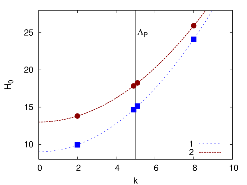
Figure 1: The kinetic energies $H_{0,i}$ as function of the momentum $k$ for the model. The line with squares denotes the first-flavor ($i=1$) channel, the other one the second-flavor ($i=2$) channel (see text for details).

III.2 ALS iteration methods

We use two different quantities to monitor the convergence of the ALS iteration methods. As a necessary convergence condition for all iteration techniques the $x_{n}$ should tend to zero for $n\to\infty$. We therefore use the norm $\left\|x_{n}\right\|$ (maximal absolute column sum norm of $x_{n}$) as function of the number of iterations $n$ as one convergence criterion. Thus, if this norm increases, the iteration method cannot converge.

At each iteration step $n$ the approximate solution

$$\sigma_{n}=\sum_{i=0}^{n}x_{i}$$ (19)

is plugged into the decoupling equation (cf. Eq. (6))

$$d_{n}=\sigma_{n}PHQ\sigma_{n}+\sigma_{n}PHP+QHQ\sigma_{n}+QHP\ ,$$ (20)

defining in this way the quantity $d_{n}$. Its norm $\left\|d_{n}\right\|$ represents a deviation (distance) from the exact solution, where the decoupling equation is exactly fulfilled. This quantity should also tend to zero for $n\to\infty$. As a second convergence criterion we calculate the eigenvalues at each iteration step by diagonalization which is surely possible for the model and monitor their behavior as function of the number of iterations.

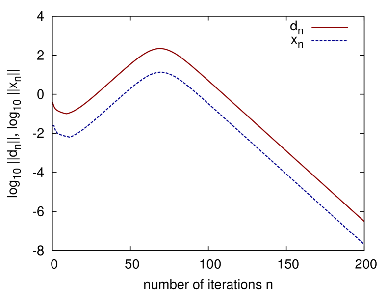
Figure 2: The norm of $x_{n}$ and of the deviation from zero $d_{n}$ of the decoupling equation for the model as function of the iteration number $n$ using the standard ALS iteration method with one momentum cutoff.

We begin our analysis with the standard ALS iteration method as described in Sec. II.1. In Fig. 2 the norm $\left\|x_{n}\right\|$ and the deviation $\left\|d_{n}\right\|$ from the exact solution of the decoupling equation are shown as a function of the iteration number $n$. After the first few iterations, these quantities increase with $n$ signaling a divergence of the method but then decrease again for a larger number of iterations. This could lead to the incorrect conclusion that the ALS iteration method converges anyway to the right eigenvalues.

This is demonstrated in the following: The eigenvalues in the $P$-space are given by the eigenvalues of $p(\sigma_{n})$ and are plotted in Fig. 3 as a function of the iteration number. The dashed lines are the final exact eigenvalues obtained by diagonalization of the model Hamiltonian.

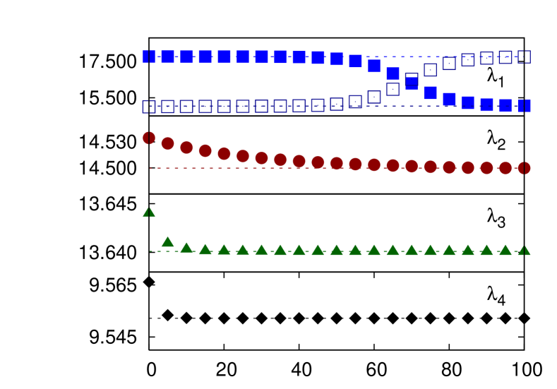
Figure 3: The $P$-space eigenvalues evolution for the model using the standard ALS iteration with one momentum cutoff. The open squares label the nearest $Q$-space eigenvalue. See text for details.

The starting values for the eigenvalues are given by $PHP=p(0)$. Due to our grid choice for the model we can identify the $P$- and $Q$-space eigenvalues uniquely. We violate in this way the convergence condition (11) because the $Q$-space eigenvalue near the cutoff is smaller than the corresponding $P$-space eigenvalue (cf. Fig. 1). Thus, we expect that the standard ALS iteration method does not converge.

This is clearly visible in Fig. 3 for the eigenvalue $\lambda_{1}$ where the evolution of the $P$-space eigenvalue (filled squared) and the corresponding $Q$-space eigenvalue (open squared) are shown. Although the $x_{n}$’s tend to zero, the eigenvalues converge for large $n$ to the ones with minimum absolute value. The $P$-space eigenvalue evolves from $\lambda_{1}\sim 17.78$ to $15.05$ and the $Q$-space one from $15.00$ to $17.76$. This mixing between a $P$- and $Q$-space eigenvalue during the decimation is typical for a divergence in the ALS iteration method. Due to our grid choice we have only one eigenvalue mixing the other three $P$-space eigenvalues converge to the correct solutions. But in general an arbitrarily larger number of eigenvalues which violate condition (11) could mix.

Unfortunately, for realistic interactions like the hyperon-nucleon interaction it is not possible to identify and sort the proper $P$- and $Q$-space eigenvalues for each $i$th-subblock. One has to find alternative criteria which signal an eigenvalue mixing. One alternative is the norms $\left\|x_{n}\right\|$ and $\left\|d_{n}\right\|$. During the mixing the $\left\|x_{n}\right\|$ and $\left\|d_{n}\right\|$ rise and once the eigenvalue sorting is completed they begin to drop again. Thus, a rising $\left\|x_{n}\right\|$ (or $\left\|d_{n}\right\|$) and a following dropping with the iteration number $n$ signals a level crossing and the standard ALS iteration method converges to wrong results. This behavior is shown in Fig. 2.

As already mentioned, the standard ALS iteration method can be modified and improved by adding a diagonal matrix $M=\operatorname{diag}(m_{1},\ldots)$ to the decoupling equation with arbitrary chosen $m_{i}$ (cf. Eq. (II.1). Then, the eigenvalues converge closest to the chosen numbers $m_{i}$. But the crucial point here is how to chose this matrix $M$? No general criterion is known. For the model calculation it is possible to try several different ansätze, which indeed prevent the mixing of the $P$- and $Q$-space eigenvalues and result in stable eigenvalues.

Unfortunately, all these ansätze cannot be applied to realistic interactions. For a realistic coupled channel calculation much more mesh points have to be taken into account. Then the identification of the $P$- and $Q$-space eigenvalues for each flavor channel $i$ is not possible any longer. This is also visible in Fig. 1. One cannot distinguish between the channel 2 $P$-space eigenvalues for small momenta $k$ and the channel 1 $P$-space eigenvalues for momenta around the cutoff $\Lambda_{P}$. Even an alternative identification of the appropriate eigenvalues by means of eigenvector distributions, as described e.g. in Ref. Fujii et al. (2004), fails for realistic multi-flavor channel interactions.

For our model the situation is different. By construction, the eigenvalues of the $P$- and $Q$-space are well-separated and can be assigned uniquely. One way out of this dilemma is the introduction of a so-called channel-dependent cutoff. The use of the channel-dependent cutoff will cure not only the identification problem of the eigenvalues but also has a natural physical interpretation which we will discuss in the following.

III.3 Channel-dependent cutoff

We assume that the dominant contribution to the full Hamiltonian comes from its kinetic energy $H_{0}$ and the interaction is a small perturbation. The channel-dependent cutoff is a general prescription how to define the model space for low-momentum interactions that include flavor transitions with different masses. This is for example of relevance for the hyperon-nucleon interaction in the particle basis Schaefer et al. . The idea of the channel-dependent cutoff is to truncate the kinetic energy of each channel to the same energy $\Lambda_{E}$. The truncation of the kinetic energy in this way leads to different momentum cutoffs in each flavor channel $\Lambda_{i}$. This is depicted in Fig. 4.

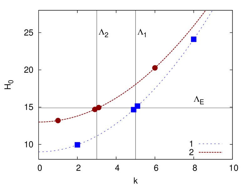
Figure 4: The kinetic energy $H_{0}$ as a function of the momentum $k$ for the model similar to Fig. 1. The line with the squares denotes the first-flavor channel, the other one the second-flavor channel.

In principle there are two possibilities how to construct the momentum cutoffs. One possibility is to fix the value of the kinetic energy $\Lambda_{E}$ and then to calculate the corresponding momentum cutoffs $\Lambda_{i}$. But the following procedure is better adapted to a generalization of the $V_{\text{low }k}$ method to multi-flavor channels. Instead of fixing the kinetic energy $a$ $priori$, one calculates its value for a given momentum cutoff of the flavor channel with the smallest mass. For our model this means to choose $\Lambda_{1}$ for channel 1 and calculate $\Lambda_{2}$ for channel 2 by requiring

$$H_{0,1}\left(\Lambda_{1}\right)=H_{0,2}{\left(\Lambda_{2}\right)}\ .$$ (21)

For example, choosing a momentum cutoff $\Lambda_{1}=\Lambda=5$ for channel 1 this results in a smaller cutoff in channel 2

$$\Lambda_{2}=\sqrt{2\mu_{2}\left(\frac{\Lambda_{1}^{2}}{2\mu_{2}}+m_{1}-m_{2}\right)}\approx 3.1\,,$$ (22)

which is denoted by the vertical line in Fig. 4. Due to the new momentum cutoff $\Lambda_{2}$ the mesh points have also changed for channel 2. A generalization to multi-flavor channels is straightforward.

Using this channel-dependent cutoff, the eigenvalues of the $P$- and $Q$-space are now clearly separated and the necessary convergence conditions (11) and (14) are fulfilled. Here, we have assumed that the potential is a perturbation and does not influence the eigenvalue sorting strongly. We have checked this assumption by a numerical calculation of the eigenvalues also in the realistic calculation.

As already mentioned, note that with only one momentum cutoff for multi-flavor channels it is not possible to fulfill these convergence conditions and the ALS iteration methods must therefore fail.

Another, more physical motivation for the channel-dependent cutoff is the following: The derivation of the $V_{\text{low }k}$ renormalization group equation is based on a Lippmann-Schwinger equation for the $T$-matrix. The propagator in the LSE is inverse proportional to the energy, which is truncated by a momentum cutoff. For channels with different reduced masses this would allow for different kinetic energies. Thus, it is natural to restrict the kinetic energy available in the propagator and not to restrict the momenta. For one-flavor channels this difference does not play any role.

This becomes more transparent if one considers an on-shell scattering process of particles with different masses. Assume the scattering of a particle of channel $2$ into a particle of channel $1$ with a relative incoming momentum around the model space cutoff, i.e. $k^{\prime}\approx\Lambda$ and masses $m_{2}>m_{1}$. Since we consider on-shell scattering, the energy

$$H_{0,2}(k^{\prime}\approx\Lambda)\approx\frac{\Lambda^{2}}{2\mu_{2}}+m_{2}=E\,.$$ (23)

is fixed, say to $E$. This would result in

$$E=H_{0,1}(k)=\frac{k^{2}}{2\mu_{1}}+m_{1}\ ,$$ (24)

for the scattered particle $1$, which in turn yields for the outgoing relative momentum

$$k=\sqrt{\mu_{1}\left(\frac{\Lambda^{2}}{\mu_{2}}+2(m_{2}-m_{1})\right)}\ .$$ (25)

Since we have assumed $m_{2}>m_{1}$ this outgoing relative momentum is larger than our cutoff $\Lambda$. For example, choosing for the incoming momentum $k^{\prime}=4.9$ the outgoing momentum would be $k\approx 7.4$. Since all momenta are limited by the cutoff $\Lambda=5$ such transitions are not allowed. This is also clearly visible in Fig. 4

Since the channel-dependent cutoff restricts the kinetic energy it can be represented by a horizontal line in this figure. One never crosses this line in any on-shell scattering process.

When we apply the channel-dependent cutoff to the model, the mesh points will change due to the different momentum cutoff, which is shown in Fig. 4. This yields also a change of the eight exact eigenvalues. In this case we find the eigenvalues $H=\operatorname{diag}(9.55,14.50,15.05,24.04,12.96,14.56,14.88,20.22)$ which are again close to the points in Fig. 4.

Due to the channel-dependent cutoff the convergence criterion for the ALS iteration methods are fulfilled now because the $P$-space eigenvalues are these eigenvalues which are closest to zero. The different iteration schemes converge monotonic and to the correct $P$-space eigenvalues. An example for the standard ALS iteration is shown in Fig. 5.

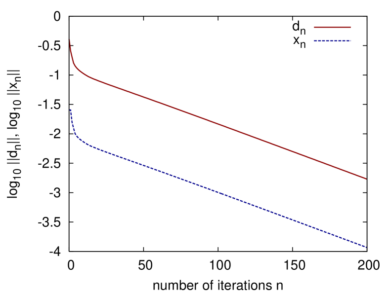
Figure 5: Same as Fig. 2 for the model using the standard ALS iteration method with a channel-dependent cutoff.

The evolution of the four $P$-space eigenvalues for the model as a function of the number of iterations is displayed in Fig. 6. The dashed lines are the exact eigenvalues. All eigenvalues converge to the correct ones. Due to the small gap between the largest $P$-space and the smallest $Q$-space eigenvalue in the model ,the number of iterations of is slightly larger compared e.g. to Fig. 3.

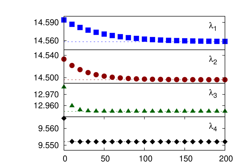
Figure 6: The $P$-space eigenvalue evolution for the model similar to Fig. 3 using the standard ALS iteration method with a channel-dependent cutoff.

IV Summary

In this work the ALS iteration methods and its modifications are investigated, which are necessary to solve coupled-channel equations with different masses. Instead of working with realistic interaction potentials, a simple and solvable model, which mimics all the relevant properties of a realistic interaction is introduced.

First, we applied the ALS iteration method and its modifications to the one-flavor channel and discussed its failure for multi-flavor channels. Due to the different masses inherent in the multi-flavor case the necessary convergence conditions are violated.

By an introduction of a channel-dependent cutoff we could generalize these ALS iteration modifications and could restore the convergence. This channel-dependent cutoff results in an effective interaction which is still energy-independent and thus preserves a major advantage of the $V_{\text{low }k}$ potential.

An on-shell scattering example of two particle with different masses provides a more physical motivation for this novel cutoff. Without the channel-dependent cutoff unphysical scattering processes out of the model space become possible. First encouraging results for a realistic hyperon-nucleon interaction by means of the channel-dependent cutoff have been published in Ref. Schaefer et al. (2006). Further calculations including a broader variety of input potentials such as the Nijmegen potentials (NSC97 Rijken et al. (1999), NSC89 Maessen et al. (1989)), Jülich potential (Juelich04 Haidenbauer and Meissner (2005)), and potentials based on chiral symmetry (LO potential  Polinder et al. (2006)) will be presented elsewhere Schaefer et al. .

References

- Bogner et al. (2003) S. K. Bogner, T. T. S. Kuo, and A. Schwenk, Phys. Rept. 386, 1 (2003), eprint nucl-th/0305035.
- Lee and Suzuki (1980a) S. Lee and K. Suzuki, Phys. Lett. 91B, 173 (1980a).
- Suzuki and Lee (1980) K. Suzuki and S. Y. Lee, Progress of Theoretical Physics 64, 2091 (1980).
- Andreozzi (1996) F. Andreozzi, Phys. Rev. C 54, 684 (1996).
- Bogner et al. (2001) S. K. Bogner, A. Schwenk, T. T. S. Kuo, and G. E. Brown (2001), eprint nucl-th/0111042.
- Navratil et al. (2000) P. Navratil, G. P. Kamuntavicius, and B. R. Barrett, Phys. Rev. C61, 044001 (2000), eprint nucl-th/9907054.
- Stetcu et al. (2005) I. Stetcu, B. R. Barrett, P. Navratil, and J. P. Vary, Phys. Rev. C71, 044325 (2005), eprint nucl-th/0412004.
- Schaefer et al. (2006) B.-J. Schaefer, M. Wagner, J. Wambach, T. T. S. Kuo, and G. E. Brown, Phys. Rev. C73, 011001 (2006), eprint nucl-th/0506065.
- Hjorth-Jensen et al. (1995) M. Hjorth-Jensen, T. T. S. Kuo, and E. Osnes, Phys. Rept. 261, 125 (1995).
- Lee and Suzuki (1980b) S. Lee and K. Suzuki, Prog. Theor. Phys. 64, 2091 (1980b).
- Rijken et al. (1999) T. A. Rijken, V. G. J. Stoks, and Y. Yamamoto, Phys. Rev. C 59, 21 (1999).
- Miyagawa and Yamamura (1999) K. Miyagawa and H. Yamamura, Phys. Rev. C 60, 024003 (1999).
- Suzuki et al. (1994) K. Suzuki, R. Okamoto, P. J. Ellis, and T. T. S. Kuo, Nucl. Phys. A567, 576 (1994), eprint nucl-th/9306022.
- Fujii et al. (2004) S. Fujii et al., Phys. Rev. C70, 024003 (2004), eprint nucl-th/0404049.
- (15) B.-J. Schaefer, M. Wagner, J. Wambach, T. T. S. Kuo, and G. E. Brown, to be published.
- Maessen et al. (1989) P. M. M. Maessen, T. A. Rijken, and J. J. de Swart, Phys. Rev. C 40, 2226 (1989).
- Haidenbauer and Meissner (2005) J. Haidenbauer and U.-G. Meissner, Phys. Rev. C72, 044005 (2005), eprint nucl-th/0506019.
- Polinder et al. (2006) H. Polinder, J. Haidenbauer, and U.-G. Meissner (2006), eprint nucl-th/0605050.