Solution of the Bohr hamiltonian for soft triaxial nuclei

Abstract

The Bohr-Mottelson model is solved for a generic soft triaxial nucleus, separating the Bohr hamiltonian exactly and using a number of different model-potentials: a displaced harmonic oscillator in $\gamma$, which is solved with an approximated algebraic technique, and Coulomb/Kratzer, harmonic/Davidson and infinite square well potentials in $\beta$, which are solved exactly. In each case we derive analytic expressions for the eigenenergies which are then used to calculate energy spectra.

Here we study the chain of osmium isotopes and we compare our results with experimental information and previous calculations.

I Introduction

The Bohr-Mottelson collective model of the nucleus has recently attracted a significant interest because of the possibility to derive many “new” solvable cases Iac1 ; Iac2 ; Iac3 ; RoBa ; Cap ; FV ; FV2 ; Pepe ; Bona1 ; Bona2 ; BonZ5 ; Mark2 ; Rowe-new ; LF ; Pietr ; CapNew ; RoI ; RoTuRe . Intense efforts did arise because of the availability of models, based on the square well potential, that are related with the issue of critical point symmetries at the shape phase transition (E(5), X(5) and Y(5)) Iac1 ; Iac2 ; Iac3 . This has given rise from one side to many applications aimed at the survey of existing experimental spectroscopic data and at the identification of signatures for the new models Cast ; Kru ; Capal ; Clark ; Tonev ; Liu ; Frank in various mass regions, especially in connection with the effort to build new descriptions for transitional nuclei. On the other side a number of mathematical solutions of the Schrödinger equation associated with the Bohr hamiltonian with various model-potentials have been proposed Cap ; FV ; FV2 ; Pepe ; Bona1 ; Bona2 ; BonZ5 ; LF ; Pietr ; CapNew ; RoI ; RoTuRe . For some of those potentials, that in general are functions of the quadrupole deformation variables $\beta$ and $\gamma$, an exact separation of variables is possible, while in other cases an approximate separation holds. Usually the spectrum (and transition rates) is derived analytically and compared with available experimental data. We like to mention that for a number of these new solvable cases extensive comparisons with experimental data are still not available.

Recently a solvable model was proposed for the soft triaxial rotor with a minimum in the potential along the $\gamma$ direction located at $\pi/6$ LF . The aim of the present paper is to extend and complete that solution, proposing a solvable model for which the Schrödinger equation is separable. The $\gamma-$angular part is then solved for a harmonic potential centered around any $\gamma_{0}$ in the interval $~{}]0,\pi/3[~{}$, while the $\beta$ part is solved exactly for the Kratzer-like potential, for the Davidson potential and for the infinite square well potential.

Another reason for the search of analytic solutions for the more general case with non-irrotational moments of inertia comes also from a recent study Wood in which the rigid triaxial rotor model is improved by relaxing the assumption of irrotational flow moments of inertia. The fit of the three components of the moment of inertia to experimental data improves the description of a number of nuclear properties and suggests that the irrotational assumption is not correct. Our model incorporates this idea and extends the rigid model to $\gamma$-soft models.

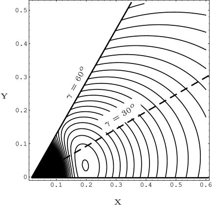
Figure 1: Contour plot of the potential $V(\beta,\gamma)$ with minimum in $\gamma_{0}=10^{o}$ and $\beta_{0}=0.2$. The situation depicted here corresponds to a very soft deformed triaxial rotor, where the $V_{1}(\beta)$ potential (see Eq. (3)) has a Kratzer-like form, while the $V_{2}(\gamma)$ is a displaced harmonic oscillator. The coordinates are $X=\beta\cos{\gamma}$ and $Y=\beta\sin{\gamma}$. In the point $\beta=0$ the potential goes to $+\infty$ (black area).

To give an idea of the typical problem that we are considering we show as an illustration in Fig. (1) a contour plot of the potential surface with a Kratzer-like potential in $\beta$ (with the minimum at $\beta_{0}=0.2$) and a displaced harmonic oscillator potential in $\gamma$ (with the minimum at $\gamma_{0}=10^{o}$). The solution of the two-dimensional Schrödinger equation for the Bohr hamiltonian containing this potential surface is given by a set of eigenvalues and their corresponding eigenstates. To each eigenstate (and in particular to the ground state) an average quadrupole shape is associated. In the present case (Fig. 1) the wave functions are concentrated around the region of the minimum and thus we are dealing with a soft triaxial rotor.

The present study may also be considered as an attempt to solve a simple model that may be compared with microscopic theories (like HF, HF+BCS or HFB) GG ; Hay ; Ansari . The potential surfaces used throughout the paper, rather than calculated with a variational procedure in a microscopic framework, are instead a priori given in analytical form. A number of early microscopic studies, like for example Ref. GG , concluded that $\gamma-$softness was not only unavoidable in triaxial nuclei, but that the potential barrier in the $\gamma$ direction was so small to cast doubts on the applicability of the rigid rotor model. We therefore reanalyze a number of osmium isotopes, which were treated within a HFB formalism, and compare our results with the results of Ref. Ansari .

In the present paper, we use a potential of the form $V_{1}(\beta)+V_{2}(\gamma)/\beta^{2}$, which allows for a separation of the Bohr hamiltonian in $\beta$ and $(\gamma,\theta_{i})$ part (Section II). The solution of the $(\gamma,\theta_{i})$ part is amply presented in Section III. In Section IV we discuss the quantum numbers associated with the present model and presents a few comments on quasidynamical symmetry. In Section V we discuss in detail some examples that illustrate the method of solving Eq. (10). In Section VI, we solve analytically the $\beta$ part of the problem in the Coulomb/Kratzer, harmonic/Davidson and infinite square well cases. In Sections VII and VIII, we discuss the fitting procedure and its accuracy and we apply the method to the chain of osmium isotopes and make a comparison with other calculations. Here, we also stress the fact that, in doing so, in general we go beyond an irrotational approach and make use of three different moments of inertia used as parameters. The need to take into account this possibility has been emphasized before by Wood et al. Wood . We also compare with the situation of irrotational flow in which a value $\gamma_{0}$ can be deduced and implies that fluctuations of the moment of inertia in the $\gamma$ direction are neglected, but the softness is included. It is interesting to notice that the values of $\gamma_{0}$ so obtained correlate well with results extracted from different methods used to analyze data in the Os nuclei (Section VIII). We analyze these isotopes, particularly because they are thought to be situated in the transitional region between $\gamma-$rigid and $\gamma-$soft shapes. In Section IX, we formulate the main conclusions of the present study, while in appendix A, we explicitly present the matrix elements used in the calculations.

II Formulation of the model

The Schrödinger equation for the Bohr hamiltonian reads

$$\hat{H}_{B}\Psi(\beta,\gamma,\theta_{\iota})~{}=~{}E\Psi(\beta,\gamma,\theta_{\iota})\,,$$ (1)

where the hamiltonian is given by

$$\hat{H}_{B}~{}=~{}-{\hbar^{2}\over 2B_{m}}{1\over\beta^{4}}{\partial\over\partial\beta}\beta^{4}{\partial\over\partial\beta}-{\hbar^{2}\over 2B_{m}}{1\over\beta^{2}}{1\over\sin{(3\gamma)}}{\partial\over\partial\gamma}\sin{(3\gamma)}{\partial\over\partial\gamma}+{\hbar^{2}\over 8B_{m}\beta^{2}}\sum_{i=1,2,3}{{\hat{L}}_{i}^{2}\over\sin^{2}(\gamma-2\pi\,i/3)}+V(\beta,\gamma)\,.$$ (2)

Here ${\hat{L}}_{i}$ are the projections of the angular momentum ($\hat{L}$) on the body-fixed axes and $B_{m}$ is the mass parameter. An exact separation of the variables $\beta$ and $\gamma$ may be achieved when the potential is chosen as

$$V(\beta,\gamma)~{}=~{}V_{1}(\beta)+{V_{2}(\gamma)\over\beta^{2}}\,.$$ (3)

The resulting set of differential equations (one containing only the $\beta$ variable and the other containing the $\gamma$ variable and the Euler angles, $\theta_{\iota}$ with $\iota=1,2,3$), after multiplication by $2B_{m}/\hbar^{2}$, reads

$$\Bigl{\{}-{1\over\beta^{4}}{\partial\over\partial\beta}\beta^{4}{\partial\over\partial\beta}+u_{1}(\beta)-\epsilon+{\omega\over\beta^{2}}\Bigr{\}}\xi(\beta)=0$$ (4)

$$\Bigl{\{}-{1\over\sin{(3\gamma)}}{\partial\over\partial\gamma}\sin{(3\gamma)}{\partial\over\partial\gamma}+\sum_{i=1,2,3}{{\hat{L}}_{i}^{2}\over 4\sin^{2}(\gamma-2\pi\,i/3)}$$

$$+u_{2}(\gamma)-\omega\Bigr{\}}\psi(\gamma,\theta_{\iota})~{}=~{}0\,,$$ (5)

where $\omega$ is the separation constant, $\epsilon=(2B_{m}/\hbar^{2})E$ and $u_{t}=(2B_{m}/\hbar^{2})V_{t}$ with $t=1,2$. The wavefunctions satisfy $\Psi(\beta,\gamma,\theta_{\iota})~{}=~{}\xi(\beta)\psi(\gamma,\theta_{\iota})$. In Ref. LF the same derivation has been proposed, but the problem was restricted to deriving the solution of the soft triaxial rotor around $\gamma\sim\pi/6$. In that case the rotational kinetic term may be written in a very simple way and the solution of $\gamma-$angular part may be given in a straightforward way. The main result of Ref. LF was, (i) to extend the Meyer-ter-Vehn formula MTV (strictly valid for a rigid rotor at $\gamma=30^{o}$) proving that the corresponding formula for the $\gamma-$soft rotor requires the addition of a (trivial) harmonic term in the $\gamma$ degree of freedom and (ii) to show that the solution of the full problem does not necessarily imply a trivial extension with some additive term to include the $\beta-$vibrations, but rather yields an expression for the energy levels in which the quantum numbers are intertwined in a more complicated way.

Here we extend the results of Ref. LF , addressing the more general problem of a soft triaxial rotor (not confined to $\gamma\sim 30^{o}$), solving approximatively the $\gamma-$angular equation with a potential of the form

$$u_{2}(\gamma)=C(\gamma-\gamma_{0})^{2}=Cx^{2}\,,$$ (6)

that has a minimum in the interval $0^{o}<\gamma_{0}<60^{o}$. For symmetry reasons we can restrict ourselves to the sector $0^{o}<\gamma_{0}\leq 30^{o}$. The obstacle to the further separation of variables in Eq. (5) is represented by the rotational term (second term), that mixes the variable $\gamma$ with the projections of the angular momentum. This term can be rewritten as $\sum_{i}A_{i}\hat{L}_{i}^{2}$. We will follow two strategies to deal with the coefficients $A_{i}$.

• The first strategy is to approximate these coefficient as follows

  $$A_{i}={1\over 4\sin^{2}(\gamma_{0}-2\pi\,i/3)}\,,$$ (7)

  and to replace the corresponding terms in Eq. (5). The physical meaning of this approximation is that the fluctuations of the moments of inertia are completely neglected, while the softness is taken into account. Making use of the form (7), we can parametrise the components of the moment of inertia by one single parameter.

• It has been shown in an extension of the rigid rotor model Wood that the components of the moment of inertia fitted to experimental data do not necessarily agree with the irrotational approximation. We will therefore include this observation in our model, as a second strategy, taking the components of the moment of inertia as parameters.

In the spirit of finding a simple solution, we introduce in Eq. (5) the further simplification $~{}\sin{3\gamma}\sim\sin{3\gamma_{0}}~{}$, obtaining

$$\Bigl{\{}\overbrace{-{\partial^{2}\over\partial x^{2}}+Cx^{2}}^{\hat{D}_{2}}-\omega+\sum_{i=1,2,3}A_{i}{\hat{L}}_{i}^{2}\Bigr{\}}\psi(x,\theta)=0\,,$$ (8)

where the variable $x$, introduced in (6), has been used and where the second order differential operator $\hat{D}_{2}$ has been defined. The wavefunction may be written in the unsymmetrized form as an expansion in terms of rotational wavefunctions, namely

$$\psi_{L,M}(x,\theta)~{}=~{}\sum_{K^{\prime}}a_{K^{\prime}}^{L}(x){\cal D}^{L}_{M,K^{\prime}}(\theta)\,.$$ (9)

where $K^{\prime}$ is introduced to distinguish the multiple occurrence of states with the same $L$. One may notice that the rotational basis has an SO(2) symmetry reflected in the good quantum number $K^{\prime}$. We now multiply to the left by ${\cal D}^{L}_{M,K}$ and integrate over the Euler angles, exploiting the orthonormality property of the Wigner functions where possible. The result is the set of equations (one for each allowed value of $K$)

$$({\hat{D}_{2}}-\omega)a^{L}_{K}(x)+\sum_{i}A_{i}\sum_{K^{\prime}}\langle LMK\mid\hat{L}_{i}^{2}\mid LMK^{\prime}\rangle a^{L}_{K^{\prime}}(x)=0\,,$$ (10)

each of which contains matrix elements of the squared components of the angular momentum (see appendix). We may rewrite it also as

$$\Bigl{(}{\hat{D}_{2}}-\omega+\sum_{i}A_{i}\langle LMK\mid\hat{L}_{i}^{2}\mid LMK\rangle\Bigr{)}a^{L}_{K}(x)+$$

$${(A_{1}-A_{2})\over 4}\langle LMK\mid\hat{L}_{+}^{2}\mid LMK-2\rangle a^{L}_{K-2}(x)+{(A_{1}-A_{2})\over 4}\langle LMK\mid\hat{L}_{-}^{2}\mid LMK+2\rangle a^{L}_{K+2}(x)=0$$ (11)

to highlight that only three of the $a$ coefficients appear in every equation.

III Algebraic approach

A convenient way to treat the $\gamma-$angular part is to consider the dynamic symmetry associated with the $\hat{D}_{2}$ operator, that is essentially a harmonic oscillator hamiltonian. The advantage here lies in the fact that the spectrum generating algebra allows us to write explicit expressions for the $\gamma-$vibrational spectrum.

The infinitesimal generators of the sp(2,$\mathbb{R}$) Lie algebra may be written as

$$\hat{Z}_{1}=-{1\over k}{\partial^{2}\over\partial x^{2}}\qquad\hat{Z}_{2}=kx^{2}\qquad\hat{Z}_{3}=-i\Bigl{(}{1\over 2}+x{\partial\over\partial x}\Bigr{)}\,,$$ (12)

where $k$ is a constant. Similar approaches have been used in Ref. RoBa ; FV . The operators above close under commutation, i.e.:

$$[\hat{Z}_{1},\hat{Z}_{2}]=-4i\hat{Z}_{3}\quad[\hat{Z}_{3},\hat{Z}_{2}]=-2i\hat{Z}_{2}\quad[\hat{Z}_{3},\hat{Z}_{1}]=2i\hat{Z}_{1}\,.$$ (13)

With the linear transformation

$$\hat{X}_{1}~{}=~{}{1\over 4}\bigl{(}\hat{Z}_{1}-\hat{Z}_{2}\bigr{)}\qquad~{}\hat{X}_{2}~{}=~{}{1\over 2}\hat{Z}_{3}\qquad~{}\hat{X}_{3}~{}=~{}{1\over 4}\bigl{(}\hat{Z}_{1}+\hat{Z}_{2}\bigr{)}\,,$$ (14)

one may recognize the standard commutation relations of the four isomorphic Lie algebrae su(1,1)$\sim$so(2,1)$\sim$sp(2,$\mathbb{R}$)$\sim$ sl(2,$\mathbb{R}$)

$$[\hat{X}_{1},\hat{X}_{2}]=-i\hat{X}_{3}\qquad~{}[\hat{X}_{2},\hat{X}_{3}]=i\hat{X}_{1}\qquad~{}[\hat{X}_{3},\hat{X}_{1}]=i\hat{X}_{2}.$$ (15)

It is also very useful to define raising, lowering and weight operators for this algebra,

$$\hat{X}_{\pm}=\hat{X}_{1}\pm i\hat{X}_{2}\qquad\hat{X}_{0}=\hat{X}_{3}\,,$$ (16)

that obey the following commutation relations

$$[\hat{X}_{+},\hat{X}_{-}]=-2\hat{X}_{0}\qquad[\hat{X}_{0},\hat{X}_{\pm}]=\pm\hat{X}_{\pm}\,.$$ (17)

The action of the above operators on orthonormal basis states for the irreps of su(1,1) ($\mid n,\lambda\rangle$ with $n=0,1,2,..$) is given by the equations:

$$\hat{X}_{+} \mid n\lambda\rangle=\sqrt{(\lambda+n)(n+1)}\mid n+1,\lambda\rangle$$ (18)

$$\hat{X}_{-} \mid n+1,\lambda\rangle=\sqrt{(\lambda+n)(n+1)}\mid n\lambda\rangle$$ (19)

$$\hat{X}_{0} \mid n\lambda\rangle={1\over 2}(\lambda+2n)\mid n\lambda\rangle\,.~{}~{}~{}~{}~{}~{}~{}~{}~{}~{}~{}~{}~{}~{}~{}$$ (20)

The values of $\lambda$ are found by comparing the standard eigenvalue equation for the Casimir operator of su(1,1) with the eigenvalue equation for the same operator, but explicitly realized in the terms of the operators defined in (12):

$$\hat{\mathbb{C}}_{2}\mid n\lambda\rangle~{}=~{}\Bigl{(}\hat{X}_{3}^{2}-\hat{X}_{1}^{2}-\hat{X}_{2}^{2}\Bigr{)}\mid n\lambda\rangle~{}=~{}{1\over 4}\lambda(\lambda-2)\mid n\lambda\rangle\,.$$ (21)

The action of the Casimir operator on a given function $\phi(x)$ gives

$$\hat{\mathbb{C}}_{2}\mid\phi\rangle=\Biggl{\{}{1\over 8}\Bigl{(}\hat{Z}_{1}\hat{Z}_{2}+\hat{Z}_{2}\hat{Z}_{1}\Bigr{)}-{\hat{Z}_{3}^{2}\over 4}\Biggr{\}}\mid\phi\rangle=-{3\over 16}\mid\phi\rangle\,.$$ (22)

Therefore we obtain $\lambda={1/2,3/2}$. As a consequence of the definitions given in this and in the previous section, we notice that

$$\hat{D}_{2}~{}=~{}\sqrt{C}(\hat{Z}_{1}+\hat{Z}_{2})~{}=~{}\sqrt{C}4\hat{X}_{0}\,,$$ (23)

where the constant $k$ is defined as $k=\sqrt{C}$. The action of the operator $4\hat{X}_{0}$ is given, for each allowed value of $\lambda$, by $(1+4n)$ and $(3+4n)$ respectively. Combining the two results we may write that the eigenvalue equation for the $\hat{D}_{2}$ operator is given by

$$\hat{D}_{2}\mid n_{\gamma}\rangle~{}=~{}\sqrt{C}(1+2n_{\gamma})\mid n_{\gamma}\rangle\,,$$ (24)

where we dropped the index $\lambda$ to cover the whole spectrum, and as $\hat{D}_{2}$ is the harmonic oscillator operator in the $\gamma-$degree of freedom, we can associate $n$ with the number of phonons in the $\gamma-$variable, $n=n_{\gamma}$.

IV Solution of coupled equations, quasidynamic symmetry, quantum numbers and band structure

We discuss here the quantum numbers that appear when solving the problem presented in the previous section. The coupled set of equations (10) contains the rotational and $\gamma-$vibrational structure through the functions $a^{L}_{K^{\prime}}$ and the operator $\hat{D}_{2}$ respectively. In the absence of $\gamma-$vibrations ($n_{\gamma}=0$), we are left with the rotational structure (see Fig. 2), which can be analyzed as following. For each $L$ there is a set of allowed $K$’s: $\{K_{i},...,K_{f}\}$ where $K_{i}=0$ and $K_{f}=L$ for $L$ even (thus we have $L/2+1$ coupled equations) and $K_{i}=2$ and $K_{f}=L-1$ for $L$ odd (giving $(L-1)/2$ equations).

For $\gamma=0$ and $\gamma=\pi/3$ the projection of the third component of the angular momentum on the intrinsic axis 3 gives a good quantum number ($K$), while for $\gamma=\pi/6$ the eigenvalue of the projection on the intrinsic axis 1 is a good quantum number ($R$). In the intermediate regions, none of them may be taken as a good quantum number. In the expansion (9) the introduction of $K^{\prime}$ as a label to distinguish between the multiple occurrence of states with the same value of $L$ is justified because it is referring to the rotational states.

It has been observed that in the triaxial region, moving from $\gamma=30^{o}$ toward $\gamma=0^{o}$, different groups of states may well be classified into bands: a first band ($0^{+},2^{+},4^{+},...$) tends to the finite axial rotor values and corresponds to $K=0$; a second band ($2^{+},3^{+},4^{+},...$) is identified by its behaviour when $\gamma\rightarrow 0$ (in Fig. 2 this group of states somewhat cluster around $\gamma\sim 10^{o}-12^{o}$); the beginning of a third band ($4^{+},5^{+},....$) is seen to escape to infinity at a quicker pace (leaving Fig. 2 at around $\gamma\sim 20^{o}$).

The experimental observation that a classification in $\beta$ and $\gamma$ bands seems an almost universal feature of nuclear spectra reinforces this choice. The labeling with the $K$ quantum number is often encountered in the literature, although for what we have said here it may not be considered adequate. We will in the following use the notation $K^{*}$ to regroup the various eigenstates into bands, which are the counterpart of the bands with good $K$, that are present in the axial cases.

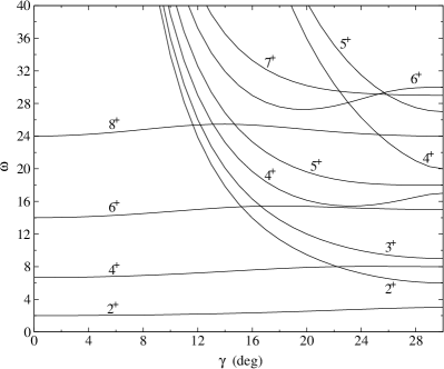
Figure 2: Eigenvalues of Eq. (10) as a function of the asymmetry for $n_{\gamma}=0$ (relative to the lowest eigenvalue). In this case the solution of the rotational part for the $\gamma-$soft triaxial rotor corresponds to the outcome of the Davydov model Davy . In addition, the soft model has infinitely many other copies (one for each possible value of $n_{\gamma}$) of these sets of bands at higher energies (depending, of course, on the magnitude of $C$).

For phonons with total angular momentum $2$, one usually takes into consideration two projections $\mid K\mid=0,2$. These projections correspond to the so-called $\beta-$ and $\gamma-$phonons, that generate axial and non-axial quadrupole oscillations, respectively. Because of the non-axial character of the $\gamma-$variable, the $\gamma-$vibrations are naturally incorporated into Eq. (10). This is obtained through the operator $\hat{D}_{2}$, which adds the $\gamma-$vibrations to the basic structure of rotations of a rigid triaxial body. Consequently, one can construct $\gamma-$bands that consist of copies of the structure of the rigid triaxial rotor (Fig. 2), where every copy possesses a different number of $\gamma-$vibrations, characterized by $n_{\gamma}$. Once the rotational and vibrational structure is determined, the eigenvalue $\omega$ can be calculated (in the standard way) and plugged into Eq. 4 to solve for the $\beta-$part of the problem. An elaborate discussion on the $\beta-$part and the chosen potentials will be addressed in section VI.

One may describe the present situation in terms of a quasidynamical symmetry RoL ; RoWi of a peculiar character: at $\gamma=0^{o}$ the group SO(2) is a symmetry of the system, associated with $K$, while at $\gamma=30^{o}$ another SO(2) group is a symmetry of the system, associated with $R$, being the chain U(5)$\supset$SO(3) common to the whole sector $0\leq\gamma\leq\pi/6$. In the intermediate region, $0<\gamma<\pi/6$, the SO(2) symmetry is broken, but it must be noticed (see Fig. 2) that the structure of the rotational spectrum, present at $\gamma=0^{o}$, persists in the whole sector without being altered in a dramatic way. Only a smooth and slight change may be seen. On the other side the structure of the ’maximally’ triaxial rotor at $\gamma=30^{o}$ persists also in the region around $\gamma\sim 20^{o}-30^{o}$. In the intermediate region these groups of states escape to infinity. It must be further noticed that the region where the various states, that originate from the axial rotor side, are most affected is exactly the region where the states coming from the $\gamma=30^{o}$ triaxial rotor diverge. The strange character of this quasidynamical symmetry is that (at variance with the cases discussed by Rowe and collaborators RoL ; RoWi ; RoI , where a true phase transition was present between two exactly solvable limits associated with different symmetries and different group structures) here we are dealing with a smooth transition between two limits which formally have the same underlying group structure, SO(2), and there is no critical point in between. Therefore we conclude that the proposed labeling, that retains the formal division in $\beta$,$\gamma$ and $K$ bands typical of an axial rotor, is not only justified by the empirical observation that non-axial nuclei display the same classification in bands, but it is also justified in view of arguments based on a group theoretical approach. It is not clear, at present, if a quantization procedure around a tilted axis may help to shed light on this aspect.

V Examples

Equation (10) is solved here in a few cases. Applying the recipe discussed in Sec. IV, the set of differential equations is turned in a single algebraic equation in $\omega$. When $L=0$, only the value $K^{\prime}=0$ is present and therefore Eq. (10) reduces to

$$\Bigl{(}\hat{D}_{2}-\omega+\sum_{i}A_{i}\langle 0\,0\,0\mid\hat{L}_{i}^{2}\mid 0\,0\,0\rangle\Bigr{)}a_{0}^{0}(x)=0\,,$$ (25)

where all the matrix elements are evaluated to be zero and the first solution is thus $\omega_{L=0,K^{*}=0,n_{\gamma}=0}=\sqrt{C}$ and we may write, in general, $\omega_{L=0,K^{*}=0,n_{\gamma}}=\sqrt{C}(1+2n_{\gamma})$.

States with $L=1$ are not present in this model.

For $L=2$, the two possibilities are $K^{\prime}=0,2$, corresponding to 2 coupled equations,

$$(\hat{D}_{2}-\omega+3A_{1}+3A_{2})a^{2}_{0}+\sqrt{3}(A_{1}-A_{2})a^{2}_{2}= 0$$

$$(\hat{D}_{2}-\omega+A_{1}+A_{2}+4A_{3})a^{2}_{2}+\sqrt{3}(A_{1}-A_{2})a^{2}_{0}= 0\,,$$

whose solutions are, $\omega_{L=2,K^{*},n_{\gamma}}=$

$$\sqrt{C}(1+2n_{\gamma})+2\sum_{i}A_{i}\pm 2\sqrt{\sum_{i}A_{i}^{2}-\sum_{i<j}A_{i}A_{j}}\,.$$ (28)

The rotational parts of these expressions reduce to the correct values, $3$ and $6$ respectively, when $\gamma=30^{o}$.

For $L=3$ the only possibility is $K^{\prime}=2$ and the solution becomes

$$\omega_{L=3,K^{*}=2,n_{\gamma}}=\sqrt{C}(1+2n_{\gamma})+4A_{1}+4A_{2}+4A_{3}\,.$$ (29)

Notice that when $\gamma=30^{o}$ two of the three components of the moment of inertia ($A_{2}$ and $A_{3}$) are equal to $1$ and the remaining ($A_{1}$) is $1/4$ so the rotational part of the energy becomes $9$ (as obtained in refs. LF and MTV ). In general we have $\omega_{L=3,K^{*}=2,n_{\gamma}}=\sqrt{C}(1+2n_{\gamma})+4\sum A_{i}$.

For $L=4$ we can write the determinant of the matrix mentioned in Sec. IV as a third degree equation in $\omega$. Its three solutions, corresponding to the cases $K^{*}=0,2,4$, may be found analytically, although their expressions are rather lengthy.

It is possible to write an algebraic equation in $\omega$ for every value of $L$, but this equation may be solved analytically only for the lowest values. We must therefore resort to numerical computation for high values of the angular momentum.

In Fig. 2 we plot the value of $\omega$ for various states for $C=0$ with irrotational moment of inertia. This case correspond to the well-known rigid rotor solution, that is a particular case of our model (see Ch. 9 of Ref. PB , for example).

Finally we notice that, as a consequence of the definitions given above, the following relation holds:

$$\omega_{200}+\omega_{220}=\omega_{000}+\omega_{320}.$$ (30)

This expression is a generalization of the well-known relation $E(2^{+})+E({2^{\prime}}^{+})=E(3^{+})$ PB .

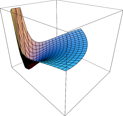
Figure 3: (Color online). Plot of $u(\beta,\gamma)$ as in formula (3) for $0\leq\gamma\leq\pi/3$. The potential $u_{1}(\beta)$ has a Kratzer-like form, while the potential $u_{2}(\gamma)$ has a displaced harmonic dependence centered around $\pi/6$ (for purpose of illustration).

VI Solution of the $\beta-$part

Once the $\gamma-$part is solved with a particular choice for the moments of inertia, we can determine the solution of the $\beta-$part inserting the appropriate values for $\omega$ in Eq. (4). With the substitution $\xi(\beta)=\chi(\beta)\beta^{-2}$, Eq. (4) is simplified to its standard form:

$${\partial^{2}\chi(\beta)\over\partial\beta^{2}}+\Bigl{\{}\epsilon-u_{1}(\beta)-{(2+\omega)\over\beta^{2}}\Bigr{\}}\chi(\beta)=0\,.$$ (31)

As shown in LF ; FV ; FV2 an interesting case is represented by the Kratzer-like potential (which reduces to a Coulomb-type potential when $B=0$)

$$u_{1}(\beta)=-A/\beta+B/\beta^{2}\,.$$ (32)

We depict in Fig. 3, as an illustration, the surface corresponding to the reduced potential $u(\beta,\gamma)=u_{1}(\beta)+u_{2}(\gamma)/\beta^{2}$ where the potential $u_{1}(\beta)$ has a Kratzer-like form, while the potential $u_{2}(\gamma)$ has a displaced harmonic dependence centered (as an example) around $\pi/6$. The depth of the pocket centered around the minimum in $(\beta_{0},\gamma_{0})$ may be adjusted with the parameters of the two potentials, $A$, $B$ and $C$.

Following LF we can write the solution to equation (4) directly as:

$$\epsilon(n_{\gamma},n_{\beta},L,K^{*})={A^{2}/4\over\Bigl{(}\sqrt{9/4+B+\omega_{L,K^{*},n_{\gamma}}}+1/2+n_{\beta}\Bigr{)}^{2}}\,,$$ (33)

where the values of $\omega_{L,K^{*},n_{\gamma}}$ have been found analytically or numerically as discussed in the previous section. Energies are usually redefined fixing the ground state to zero and using the energy of the first $2^{+}$ state as unit, namely

$$\bar{\epsilon}(n_{\gamma},n_{\beta},L,K^{*})={\epsilon(n_{\gamma},n_{\beta},L,K^{*})-\epsilon(0,0,0,0)\over\epsilon(0,0,2,0)-\epsilon(0,0,0,0)}~{}~{}.$$ (34)

Another interesting case that also leads to a solvable differential equation is the Davidson potential Elli ; Elli2 ; RoBa :

$$u_{1}(\beta)=A_{D}\beta^{2}+{B_{D}\over\beta^{2}}\,.$$ (35)

This is an extension of the harmonic potential (that can be obtained when $B_{D}=0$). Inserting this potential in Eq. (4) gives formally the Laguerre differential equation and the spectrum may be written as

$$\epsilon_{D}(n_{\gamma},n_{\beta},L,K^{*})=\sqrt{A_{D}}\Bigl{(}2n_{\beta}+\widetilde{\tau}_{L,K^{*},n_{\gamma}}+5/2\Bigr{)}\,,$$ (36)

where, dropping the indices for simplicity, $\widetilde{\tau}$ is the solution of $\widetilde{\tau}(\widetilde{\tau}+3)=B_{D}+\omega$. The redefinition in reduced energy units takes in this case a very compact form:

$$\bar{\epsilon}_{D}(n_{\gamma},n_{\beta},L,K^{*})={2n_{\beta}+\widetilde{\tau}_{L,K^{*},n_{\gamma}}-\widetilde{\tau}_{0,0,0}\over\widetilde{\tau}_{2,0,0}-\widetilde{\tau}_{0,0,0}}.$$ (37)

The combination of the results for the $\gamma-$part in Sec. IV-V and the results for the $\beta-$part yields spectra with an ample range of different possible behaviours.

Another interesting case is inspired by the E(5) and X(5) solutions Iac1 ; Iac2 . Starting again from Eq. (4) one can adopt a different substitution, namely $\phi(\beta)=\beta^{3/2}\xi(\beta)$, and a change of variables, $z=\sqrt{\epsilon}\beta$. These transformations, together with the choice of the potential as an infinite square well, yield the Bessel differential equation

$$\phi^{\prime\prime}+{\phi^{\prime}\over z}+\Bigl{(}1-{\omega+9/4\over z^{2}}\Bigr{)}\phi=0\,.$$ (38)

The solution of the equation above is given in terms of Bessel J functions of irrational order

$$\phi_{s,\omega}(\beta)=c_{s,\omega}J_{\sqrt{\omega+9/4}}\Bigl{(}x_{s,\omega}{\beta\over\beta_{w}}\Bigr{)}\,,$$ (39)

where $c_{s,\omega}$ are normalization constants (given analytically in compe ). The boundary condition at the wall of the potential well, $\phi(\beta_{w})=0$, implies that the spectrum is given by

$$\epsilon_{SQ}(n_{\beta},n_{\gamma},L,K^{*})=\Bigl{(}{x_{s,\omega}\over\beta_{w}}\Bigr{)}^{2}\,.$$ (40)

Here and in Eq. (39), $x_{s,\omega}$ is the s-th zero of the Bessel function with index that depends on $\omega_{L,K^{*},n_{\gamma}}$. Notice that $n_{\beta}=s$. The reduced spectrum takes the following form

$$\bar{\epsilon}_{SQ}(n_{\beta},n_{\gamma},L,K^{*})={x_{s,\omega_{L,K^{*},n_{\gamma}}}^{2}-x_{0,\omega_{000}}^{2}\over x_{0,\omega_{200}}^{2}-x_{0,\omega_{000}}^{2}}\,.$$ (41)

This solution is somewhat similar to the so-called Z(5) solution BonZ5 where an infinite square well in $\beta$ was combined with a harmonic oscillator centered around $\gamma=30^{o}$. Major differences are the choice of exact separation of variables made here, the extension of the solution to the whole sector $0^{o}<\gamma<60^{o}$ and the possibility to relax the hypothesis of irrotational motion in deriving for the components of the moments of inertia.

VII Random walk fitting procedure

We are now equipped with a procedure to calculate the eigenvalues of the $\gamma-$part of the problem and we have given a few analytic solutions (Coulomb and Kratzer, harmonic and Davidson, and infinite square well) for the $\beta-$part. The energy spectrum (33) depends formally on six parameters, $A,B,C,A_{1},A_{2},A_{3}$, three of which come from the potentials (32) and (6), and the other three are the components of the moment of inertia. A closer look to Eq. (34) reveals that, once the eigenspectrum is scaled in the standard way, it does not really depend on $A$, while (33) does. We can now follow the strategy to keep the irrotational hypothesis and, since the various components of the moments of inertia are connected to each other by means of the relations in (7), one has to deal with just one component (or alternatively with $\gamma_{0}$). The other two components may be thus determined inverting Eq. (7):

$$\gamma_{0}=arcsin\Bigl{(}{1\over 2\sqrt{A_{3}}}\Bigr{)}\,,$$ (42)

and, substituting the value of $\gamma_{0}$ in the definitions of $A_{1}$ and $A_{2}$, we obtain the results

$$A_{1}~{}=~{}{4A_{3}\over\Bigl{(}\sqrt{12A_{3}-3}+1\Bigr{)}^{2}}\,,\qquad A_{2}~{}=~{}{4A_{3}\over\Bigl{(}\sqrt{12A_{3}-3}-1\Bigr{)}^{2}}\,.$$ (43)

Therefore our model, using the Kratzer potential, has only three parameters, $B$, $C$ and $A_{3}$, that may be used to fit experimental energy spectra.

This reduction of parameters, though convenient, may be very restrictive (see Wood ) and we prefer to implement also a procedure to keep all the components as independent parameters, at the price of complicating the fit to experimental data. We distinguish the fitting procedures with the words irrotational (3 parameters) and non-irrotational fit (5 parameters).

Similar considerations apply to the energy spectrum of the harmonic/Davidson potential. In Eq. (36) six parameters are formally present, but using the reduced spectrum and the relations among the components of the moment of inertia, one is lead to a dependence on three of them only ($B_{D}$, $C$ and $A_{3}$). Alternatively the non-irrotational fit includes 5 parameters ($B_{D}$, $C$, $A_{1}$, $A_{2}$ and $A_{3}$). Likewise, for the square well case, (4) 2 parameters are present in the (non-)irrotational fit.

Due to the number of parameters we have preferred to use a numerical method based on a random walk procedure in order to determine the energy spectrum.

As a first step we consider an isotope and a subset of its experimental levels (usually quite small, 4 levels typically). Starting from some initial set of parameters (typically $B=C=20$ and $A_{3}=1$), we minimize the deviation of the calculated and experimental energy values by walking randomly in a suitable part of the many-dimensional parameter space. The random walk is initially constrained to take only irrotational moment of inertia (i.e. $A_{1}$ and $A_{2}$ are calculated directly from $A_{3}$) and consists of a coarse-grain and a fine-grain stage, each of which takes a certain number of steps. The coarse and the fine phases of the procedure differ in the percentual amount of the initial parameter values which is allowed to change randomly (50% and 10% typically). We usually end up with a set of parameters that correspond to some local minimum of our hypersurface (although it must be noticed that in this way we are not sure to catch the absolute global minimum). From this set one may calculate a spectrum, which can be compared with the experimental one and a total error, $\sqrt{\sum_{i}(1-E_{i}^{th}/E_{i}^{exp})^{2}}$, that gives an idea of the accuracy of the description that one may get. Usually, using as input values energies of the ground and $\gamma-$bands, the typical accuracy may range from 1% to 0.1%. At this point one is still allowed to identify a value of $\gamma_{0}$, calculated from the irrotational moments of inertia (42), with the angular position of the minimum. As a final step we start from the set of parameters resulting from the irrotational fit, but now we relax the irrotational hypothesis, treating all the components of the moment of inertia as individual parameters. Often the higher freedom of this fit reduces the error by a factor 2-10, but sometimes this procedure does not improve substantially the quality of the fits. It has to be stressed that at this point the identification with a single value for $\gamma_{0}$ does not make sense anymore.

Our goal is, from one side, to give a simple model that goes beyond the estimate of ground state energies and furnishes a decent description of ground and $\gamma-$bands, and, from the other side, allows one to extract a possible behaviour of the potential energy surface associated with a given isotope.

One must keep in mind that this model will work only when the potential energy surface has just one minimum. The fact that, after fitting, some important discrepancies result between calculated and experimental values may point out that a geometrical model may not be well applicable after all.

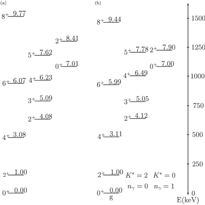
Figure 4: Experimental spectrum of ${}^{188}Os$ (a) and irrotational fit (b) obtained with $B_{D}=62.301,C=82.66,A_{3}=2.3917$. Experimental data are taken from NDS .

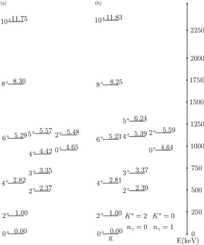
Figure 5: Experimental spectrum of ${}^{192}Os$ (a) and irrotational fit (b) obtained with $B_{D}=132.182,C=44.6504,A_{3}=1.39954$. Experimental data are taken from NDS .

VIII The osmium isotopes

We applied the procedure explained in the previous section to the case of the osmium isotopes with $A=172-180,184-192$. The irrotational fit with the Davidson potential, starting from the $4^{+}$ and $6^{+}$ levels of the ground state band and the $2^{+}$ level of the $K^{*}=2,n_{\gamma}=0$ band and the $0^{+}$ level of the $K^{*}=0,n_{\gamma}=1$ band, leads very quickly to a set of parameters ${B_{D},C,A_{3}}$ that gives always a rather good description of the low-lying positive parity energy spectrum, with an estimate on the total error, as defined above, which is in the range $0.01-0.09$. In figs. 4,5 we compare the experimental energy levels of $~{}^{188,192}$Os (a) with the irrotational fit (b), obtained from 1600 runs of coarse grained random walk plus 1600 runs of fine grained random walk. In this case the non-irrotational fit does not improve in a sizable way the quality of the fit. The absolute error in the case of the $10^{+}$ state is $\simeq 100~{}$keV, or less. In the best cases the accuracy for the $8^{+}$ and $10^{+}$ members of the ground state band may reach the value $1/1000$. It is observed that the ground-state and excited bands are fairly well reproduced (which is not surprising since we used the positions of two levels of each band as an input to our calculations). A bit more surprising is the qualitative behaviour of other bands: usually we find that the $(K^{*}=0,n_{\gamma}=1,n_{\beta}=0)$ and $(K^{*}=4,n_{\gamma}=0,n_{\beta}=0)$ bands lie lower (in a few cases dramatically lower) than the first $\beta-$band $(K^{*}=0,n_{\gamma}=0,n_{\beta}=1)$. In Fig. (6) we report the reduced energy of the bandheads of the lowest bands for the whole chain. In the osmium nuclei with lower mass number, we find comparable energies for the $\beta-$band and for the $K^{*}=0$ band, while the $K^{*}=4$ lies at considerably higher energies. This is reflected in the magnitudes of the $B_{D}$ and $C$ coefficients: for ¹⁹²Os they are respectively, $\sim 130$ and $\sim 44$, but as soon as we move to lower mass numbers the value of $B_{D}$ drops to less than $1$ for the lightest ones. Thus, the $\beta-$vibrations are found at much lower energies.

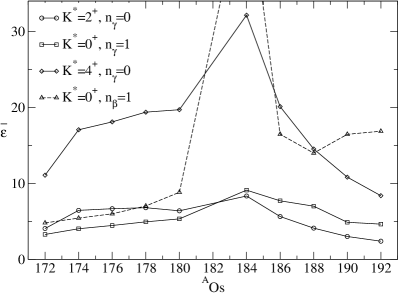
Figure 6: Reduced energies of the bandheads of the $(K^{*},n_{\gamma},n_{\beta})=$ $(2,0,0)$, $(0,1,0)$, $(4,0,0)$ and $(0,0,1)$ bands (indicated with circles, squares, diamonds and triangles respectively)as obtained from the irrotational fit procedure for the whole chain of osmium isotopes.

The example displayed in Fig. 4 is rather rigid and the (dimensionless) values of the parameters are $B_{D}=62.3$, $C=82.66$ and $A_{3}=2.3917$. The latter corresponds to a value of $\gamma_{0}\simeq 18.86^{o}$. The energy difference between the minimum of the harmonic oscillator and the values at one of the borders of the $\Delta\gamma=60^{o}$ wedge is roughly

$${\hbar^{2}\over 2B_{m}}C{(\gamma-\gamma_{0})^{2}\over\beta_{0}^{2}}\sim{0.44\over\beta_{0}^{2}}MeV\,,$$ (44)

which, for a reasonable value of $\beta_{0}$ (e.g. values smaller than 0.3), is higher than the excitation energy of the higher lying states shown in Fig. 4: $E_{8^{+}}\sim 1.5MeV$. In order to calculate the value in Eq. (44) we used the Bohr-Mottelson prescription BM for the mass coefficient, $B_{m}={1\over\lambda}{3\over 4\pi}AM_{N}R_{0}^{2}\,,$ where $\lambda=2$, $M_{N}$ is the nucleon mass and $R_{0}=r_{0}A^{1/3}$ is the nuclear radius. Therefore we obtain

$${\hbar^{2}\over 2B_{m}}={4\pi\hbar^{2}c^{2}\over 3M_{N}c^{2}r_{0}^{2}A^{5/3}}\sim{120.72MeV\over A^{5/3}}\,.$$ (45)

This expression, combined with the proper mass number, has been used in Eq. (44). The evaluation of the depth of the potential well gives an indication that the wavefunctions of the states that we have fitted are all well confined inside the well. In fact the true shape of the potential is thought to depend on $\gamma$ periodically (terms like $\cos{3\gamma}$ are the most important), therefore the harmonic oscillator shape can only represent a convenient approximation which is valid around the minimum.

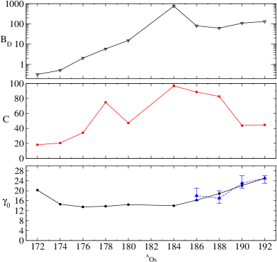
Figure 7: Values of $\gamma_{0}$ from irrotational fit to various osmium isotopes (line with circles, lower panel) and corresponding values of the parameter $C$ (middle panel) and $B_{D}$ (upper panel). Predictions obtained in Werner with a different method are also shown (dashed line, lower panel).

We show in Fig. 7 the values of $\gamma_{0}$ (black dots) obtained from the irrotational fit for the whole chain of osmium isotopes that we have analyzed together with the corresponding values of the parameter $C$ (red squares, middle part) and $B_{D}$ (diamonds, upper part). We notice that, while the value of $\gamma_{0}$ decreases from the left to the middle and then increases, the value of the parameter $C$ does not show any regular behaviour with the mass number. When one considers the extremes of the mass chain, the rotor becomes softer. By applying relation (44) to the softest case (${}^{172}Os$) one can check that the harmonic approximation is still valid.

In Fig. 7, we also display (dashed line with blue triangles) predicted effective values of $\gamma$ using $K$ shape invariants Werner . Despite the different technique used to obtain those values (which are extracted using quadrupole matrix elements and $B(E2)$ values) they agree fairly well with our results. For these values, the error bars result from errors on the measurement of the transition rates. In our case an estimate of the theoretical error is quite difficult: in principle we can repeat the fitting procedure many times and we can extract a distribution of values of parameters. To understand if our procedure is reliable we have repeated the fit on $~{}^{178}$Os 20 times. We have collected the various sets of parameters and we present in Fig. 8 the extracted values of $\gamma_{0}$. It is therefore possible to obtain an estimate of the distribution of $\gamma_{0}$ values and to give mean values and corrected standard deviations as a simple estimate for the theoretical error.

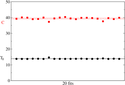
Figure 8: (Color online). Values of $\gamma_{0}$ (black dots) and of the parameter C (red squares) extracted from 20 independent fits to $~{}^{178}$Os. From these data one obtains an estimate of the theoretical error associated with the fitting procedure described in the text. Mean values, $\langle\gamma_{0}\rangle$, and mean values $\pm$ the corrected standard deviation, $(\langle\gamma_{0}\rangle\pm\sigma_{\langle\gamma_{0}\rangle})$, are indicated with dashed and dotted lines for both quantities, respectively.

Hartree-Fock-Bogoliubov calculations have been carried out (Ref. Ansari ) in the Os-Pt region with results pointing toward a prolate structure with $\gamma_{0}$ very close to $0^{o}$ and with a flat potential in $\gamma$ (for the Os nuclei with $A=186-192$). In such self-consistent calculations the potential energy surface is calculated variationally, starting from a given effective interaction. In most cases no dynamical calculations are done on top of that and energies are often associated with the exact value of the minimum of this surface. Likewise, a few excited states can also be predicted. Our approach starts from a given mathematical expression for the potential $V(\beta,\gamma)$, which is then used to solve the collective model and can predict full energy spectra. However, the particular choice of $V(\beta,\gamma)$ made at present may still deviate from actual, more realistic, potential energy surfaces. Besides, indications exist for ground state hexadecapole deformation in the Pt-Os region, as suggested by strong E4 coupling arising in $(\alpha,\alpha^{\prime})$ and $(p,p^{\prime})$ reactions.

Very recently a description of Os isotopes (among others) has been proposed within the IBM-1 Mac . The authors fit the low-energy positive-parity spectra obtaining a good overall description. Both their work and ours, which rely on models based on different ingredients, describe equally well a good fraction of the spectral properties of Os isotopes, although a number of differences clearly leave room for more detailed studies. Another analysis of quadrupole moments, transition and transfer rates of (platinum and) osmium isotopes in terms of IBM-2 bij shows that a reasonably good agreement with experimental data can be obtained with a smoothly varying set of parameters.

In our present study to construct solutions to the Bohr hamiltonian for soft triaxial nuclei, the model parameters used determine (i) the moments of inertia (through the parameter $A_{3}$, or $A_{i}$ for the more general fit), (ii) the stiffness parameter $C$ for the $\gamma-$oscillatory motion and (iii) $B_{D}$ and $A_{D}$ determining the Davidson potential. There appear rather large variations in particular in $B_{D}$ and $C$; however, the deduced value of the quantity $\gamma_{0}$ (see fig. 7 - lower part) still exhibits a very smooth variation and agrees very well with results using a totally different approach Werner . We stress that the above variations do not at all contradict the fact that smooth variations in the parameters for the IBM-2 hamiltonian result in describing the observed data in the Os nuclei, because totally different models are used.

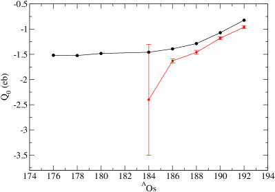
Figure 9: (Color online). Electric quadrupole moments for osmium isotopes in $eb$. Data (red squares with error bars) are taken from Ref. Ragh . The calculated values (black dots) have been obtained by adjusting an additional parameter to reproduce the excitation energy of the first $2^{+}$ state.

In order to test even further our model, we present in fig. 9 a comparison of calculated and experimental static quadrupole moments of the first excited $2^{+}$ state. The definition of the quadrupole moment adapted to the present case is:

$$Q=\sqrt{16\pi\over 5}\biggl{(}{2\atop 2}{2\atop 0}{2\atop-2}\biggr{)}{3ZR_{0}^{2}\over 4\pi}\langle 2_{1}^{+}\mid\mid\alpha_{2}^{*}\mid\mid 2_{1}^{+}\rangle$$ (46)

where the reduced matrix element, once we exploit the trigonometrical simplification for the $\gamma$ part and we insert the values of the Clebsch-Gordan coefficients, is calculated to be

$$\langle 2_{1}^{+}\mid\mid\alpha_{2}^{*}\mid\mid 2_{1}^{+}\rangle=\langle\xi_{0}(\beta)\mid\beta\mid\xi_{0}(\beta)\rangle{10\over\sqrt{70}}\bigl{(}1-{1\over 4C}\bigr{)}$$

$$\bigl{[}\cos{\gamma_{0}}(a_{2}^{2}-a_{0}^{2})+2a_{0}^{2}a_{0}^{2}\sin{\gamma_{0}}\bigr{]}\,.$$ (47)

The last expression still contains the matrix element of $\beta$ that depends on the Davidson ground state wavefunction, which in turn contains the parameter $A_{D}$. This parameter can be fixed by requiring that $\epsilon_{D}(2^{+})-\epsilon_{D}(0^{+})$ matches with the absolute energy difference in MeV. The results collected in fig. 9, are correct both in sign and trend, but they underestimate a bit the measured values Ragh . A more complete study, including $B(E2)$ values, is in progress.

IX Conclusions

In the present paper, we have presented a method in order to solve the Bohr-Mottelson collective model for a general soft triaxial nucleus. By choosing a potential of the form $V(\beta,\gamma)=V_{1}(\beta)+V_{2}(\gamma)/\beta^{2}$, the Bohr Hamiltonian separates exactly in the $\beta$ and $\gamma$ variables. Using a displaced harmonic oscillator potential in the $\gamma$ direction, representing the softness in the $\gamma$ variable, allows us to solve approximately the $\gamma$-angular equation. In solving that part of the problem, we discuss two possibilities to further separate the $\gamma$ variable from the projections of the angular momentum. One approximation neglects fluctuations of the moments of inertia in the $\gamma$ direction, but keeps the softness. Under this assumptions, the three components of the moment of inertia are related and result in one parameter. The other approximation allows a fitting of the three components of the moment of inertia independently. This is in line with the observation that the experimental data do not agree so well with the assumption of irrotational flow. We then present an algebraic method in order to find approximate solutions to the set of coupled equations that result for the motion in the $\gamma$ variable and also discuss at some length the state labeling problem in order to characterize the various collective bands that result. We subsequently study the equation for the $\beta$ degree of freedom, which can be solved exactly for a number of interesting potentials. We thus consider the Coulomb/Kratzer potential, the Davidson potential (which is an extension of the harmonic oscillator potential in $\beta$) as well as the infinite square-well potential in our calculations. In each case, we are able to derive analytic expressions, which are then used to determine the full energy spectra. These energy spectra, that describe oscillatory behavior in both the $\beta$ and $\gamma$ variables, as well as the rotational motion, in general depends on 6 parameters: three that characterize the $V(\beta,\gamma)$ potential and three that determine the moment of inertia. Using appropriate scaling in the energy spectrum only 5 remain to be determined. Going back to irrotational motion, the three components of the moment of inertia are related and this reduces the full set to just 3 parameters. Due to the number of parameters and the very involved energy eigenvalue expression, we have used a numerical method based on a random walk procedure in order to obtain the optimal fitting parameter set. We have used this method to study the Osmium isotopes in the interval $172\leq A\leq 192$. One of the results is the fact that the equilibrium $\gamma_{0}$ value shows a rather smooth dependence on $A$, but the stiffness of the potential in the $\gamma$ variable indicates rigid cases for intermediate masses and softer cases for isotopes sitting at the extremes of the considered mass chain. To elucidate this point it would be very helpful to search for solutions of Eq. (5) with more involved periodic potentials Stij . Still, the calculated values of $\gamma_{0}$ are in rather good agreement with an independent approach to extract an effective $\gamma$ value by Werner et al.. We have in mind to study the rare-earth region in a more systematic way using the methods presented here.

Recently other works have appeared that treat similar problems, yet with different spirit and aims. Caprio CapNew analyzes the numerical diagonalization of a $\beta-$soft, $\gamma-$stabilized problem, evidencing how the approximate separation of variables of the X(5) model may be questioned on the basis of a strong $\beta-\gamma$ coupling. Despite the fact that our approach is complementary (rather than solving exactly the numerical problem, we postulate analytically solvable potentials and we try to see if they can be profitably used), we reach similar conclusions. For example we also find that a considerable degree of dynamical $\gamma-$softness is needed (for realistic cases of $\gamma$ stiffness) to account for the energies of the $\gamma-$bands’ levels. Furthermore our method allows to look for the optimal value of the actual moments of inertia. A point of difference is, instead, the pattern for the staggering: in the examples below we rather find a scheme of the type $(2^{+},3^{+}),(4^{+},5^{+}),...$ similar to that of the rigid triaxial rotor. Another very important series of paper by Rowe and collaborators Rowe-new ; RoI ; RoTuRe furnishes a rapidly converging method for exact numerical treatment of the problem by using a basis defined in terms of “deformed” wavefunctions in $\beta$ and five-dimensional spherical harmonics.

The authors are most grateful to J.Wood for extensive discussions and L.F. wishes to thank A.Vitturi for profound comments. Financial support from the ”FWO Vlaanderen” (L.F. and K.H.) and the University of Ghent (S.D.B. and K.H.), that made this research possible, is acknowledged.

APPENDIX: Matrix elements

List of non-null matrix elements of operators as discussed in Eq. (11) of Sect. II.

$$\langle LMK\mid\hat{L}_{3}^{2}\mid LMK^{\prime}\rangle=K^{2}~{}~{}~{}\mbox{~{}~{}if~{}~{}}K=K^{\prime}$$ (48)

$$\langle LMK\mid\hat{L}_{1}^{2}\mid LMK^{\prime}\rangle=\left\{\begin{array}[]{lr}\displaystyle{L(L+1)-K^{2}\over 2}&~{}~{}~{}\mbox{~{}~{}if~{}~{}}K^{\prime}=K\\ \displaystyle{\langle LMK\mid\hat{L}_{+}^{2}\mid LMK^{\prime}\rangle\over 4}&~{}~{}~{}\mbox{~{}~{}if~{}~{}}K^{\prime}=K-2\\ \displaystyle{\langle LMK\mid\hat{L}_{-}^{2}\mid LMK^{\prime}\rangle\over 4}&~{}~{}~{}\mbox{~{}~{}if~{}~{}}K^{\prime}=K+2\\ \end{array}\right.$$ (49)

$$\langle LMK\mid\hat{L}_{2}^{2}\mid LMK^{\prime}\rangle=\left\{\begin{array}[]{lr}\displaystyle{L(L+1)-K^{2}\over 2}&~{}~{}~{}\mbox{~{}~{}if~{}~{}}K^{\prime}=K\\ \displaystyle-{\langle LMK\mid\hat{L}_{+}^{2}\mid LMK^{\prime}\rangle\over 4}&~{}~{}~{}\mbox{~{}~{}if~{}~{}}K^{\prime}=K-2\\ \displaystyle-{\langle LMK\mid\hat{L}_{-}^{2}\mid LMK^{\prime}\rangle\over 4}&~{}~{}~{}\mbox{~{}~{}if~{}~{}}K^{\prime}=K+2\\ \end{array}\right.$$ (50)

where

$$\langle LMK\mid\hat{L}_{+}^{2}\mid LM(K-2)\rangle=\sqrt{(L+K)(L+K-1)(L-K+2)(L-K+1)}$$ (51)

and

$$\langle LMK\mid\hat{L}_{-}^{2}\mid LM(K+2)\rangle=\sqrt{(L+K+2)(L+K+1)(L-K-1)(L-K)}~{}\,.$$ (52)

References

- (1) F.Iachello, Phys.Rev.Lett. 85, 3580 (2000).
- (2) F.Iachello, Phys.Rev.Lett. 87, 052502 (2001).
- (3) F.Iachello, Phys.Rev.Lett. 91, 132502 (2003).
- (4) D.J.Rowe and C.Bahri, J.Phys.A:Math.Gen. 31, 4947 (1998).
- (5) M.A.Caprio, Phys.Rev. C65, 031304(R) (2003).
- (6) L.Fortunato and A.Vitturi, J.Phys.G: Nucl.Part.Phys. 29 1341-1349 (2003).
- (7) L.Fortunato and A.Vitturi, J.Phys.G: Nucl.Part.Phys., 30, 627 - 635 (2004).
- (8) G.Lévai and J.M.Arias, Phys.Rev. C69, 014304 (2004).
- (9) D.Bonatsos, D.Lenis, N.Minkov, P.P.Raychev, P.A.Terziev, Phys.Rev. C69, 014302 (2004).
- (10) D.Bonatsos, D.Lenis, N.Minkov, P.P.Raychev, P.A.Terziev, Phys.Rev. C69, 044316 (2004).
- (11) D.Bonatsos, D.Lenis, D.Petrellis and P.A.Terziev, Phys.Lett. B 588, 172-179 (2004).
- (12) M.A.Caprio, Phys.Rev. C68 054303 (2003).
- (13) D.J.Rowe, Nucl.Phys. A735, 372-392 (2004).
- (14) L.Fortunato, Phys.Rev.C 70, 011302(R) (2004).
- (15) N.Pietralla and O.M.Gorbachenko, Phys.Rev. C70, 011304(R) (2004).
- (16) M.Caprio, Phys.Rev. C 72, 054323 (2005).
- (17) D.J.Rowe, Nucl.Phys. A745, 47-78 (2004).
- (18) D.J.Rowe, P.S.Turner and J.Repka, J.Math.Phys 45, 2761 (2004).
- (19) R.F.Casten and N.V.Zamfir, Phys. Rev. Lett. 85, 3584-3586 (2000); ibid., Phys.Rev.Lett. 87, 052503 (2001).
- (20) R.Krücken et al., Phys.Rev.Lett. 88, 232501 (2002).
- (21) M.A.Caprio et al., Phys.Rev.C 66, 054310 (2002).
- (22) R.M.Clark et al., Phys.Rev.C 68, 037301 (2003); R.M.Clark et al., Phys.Rev.C 69, 064322 (2004).
- (23) D.Tonev et al., Phys.Rev.C 69, 034334 (2004).
- (24) D.-l. Zhang and Y.-x. Liu, Phys.Rev.C 65, 057301 (2002).
- (25) A.Frank, C.E.ALonso and J.M.Arias, Phys.Rev.C 65, 014301 (2002).
- (26) J.L.Wood, A-M.Oros-Peusquens, R.Zaballa, J.M.Allmond and W.D.Kulp, Phys.Rev.C 70, 024308 (2004).
- (27) M.Girod and B.Grammaticos, Phys.Rev.Lett. 40, 361, (1978).
- (28) A.Hayashi, K.Hara and P.Ring, Phys.Rev.Lett. 53, 337 (1984).
- (29) A.Ansari, Phys.Rev.C 38, 953 (1988); ibid. Phys.Rev.C 33, 321 (1986).
- (30) J.Meyer-ter-vehn, Nucl.Phys. A249, 111 (1975).
- (31) A.S.Davydov and G.F.Filippov, Nucl.Phys. 8 (1958), 237.
- (32) D.J.Rowe, Phys.Rev.Lett. 93, 122502 (2004).
- (33) D.J.Rowe, C.Bahri and W.Wijesundera, Phys.Rev.Lett. 80, 4394 (1998); C.Bahri, D.J.Rowe and W.Wijesundera, Phys.Rev.C 58, 1539 (1998).
- (34) J.M.Eisenberg and W.Greiner, Nuclear Models, 2nd Ed., North-Holland Publishing Company (1975).
- (35) M.A.Preston and R.K.Badhuri, Structure of the nucleus, Addison-Wesley Publishing Company (1975), ch. 9.
- (36) J.P.Elliott, J.A.Evans and P.Park, Phys.Lett. 169B, 309 (1986).
- (37) J.P.Elliott, P.Park and J.A.Evans, Phys.Lett. B171, 145-147, (1986).
- (38) L.Fortunato, Eur.Phys.J. A26, s01 (2005).
- (39) E.Browne, Nuclear Data Sheets 72, 221-296 (1994).
- (40) Å.Bohr and B.R.Mottelson, Nuclear Structure II, World Scientific (1999, reprinted).
- (41) V.Werner, C.Scholl and P. von Brentano, Phys.Rev.C in press; ibid. EPJA, Proceedings of ENAM’04 conference, in press.
- (42) E.A.McCutchan and N.V.Zamfir, Phys.Rev.C 71, 054306 (2005).
- (43) R.Bijker, A.E.L.Dieperink, O.Scholten and R.Spanhoff, Nucl.Phys. A344 207 (1980)
- (44) P.Raghavan, At. Nucl. Data Tabl. 42, 189 (1989).
- (45) S.De Baerdemacker, L.Fortunato, V.Hellemans and K.Heyde, Nucl.Phys. A769, 16-34 (2006).