Study of the effect of the tensor correlation in oxygen isotopes with the charge- and parity-projected Hartree-Fock method

Abstract

Recently, we developed a mean-field-type framework which treats the correlation induced by the tensor force. To exploit the tensor correlation we introduce single-particle states with the parity and charge mixing. To make a total wave function have a definite charge number and a good parity, the charge number and parity projections are performed. Taking a variation of the projected wave function with respect to single-particle states a Hartree-Fock-like equation, the charge- and parity-projected Hartree-Fock equation, is obtained. In the charge- and parity-projected Hartree-Fock method, we solve the equation selfconsistently. In this paper we extend the charge- and parity-projected Hartree-Fock method to include a three-body force, which is important to reproduce the saturation property of nuclei in mean-field frameworks. We apply the charge- and parity-projected Hartree-Fock method to sub-closed-shell oxygen isotopes (¹⁴O, ¹⁶O, ²²O, ²⁴O, and ²⁸O) to study the effect of the tenor correlation and its dependence on neutron numbers. We obtain reasonable binding energies and matter radii for these nuclei. It is found that relatively large energy gains come from the tensor force in these isotopes and there is the blocking effect by occupied neutron orbits on the tensor correlation.

I Introduction

The tensor force plays important roles in nuclear structure. The study of nuclear matter using the Brueckner theory showed that the tensor force is closely related to the binding mechanism and the saturation property of nuclear matter bethe71 . The almost exact calculations with very large model spaces exhibit a large attractive energy comes from the tensor force akaishi86 ; kamada01 . The tensor force is inferred to be responsible for about a half of the single-particle spin-orbit splitting in light nuclei terasawa60 ; ando81 ; myo05 .

Recently due to the development of experimental techniques, we can access to various kinds of unstable nuclei experimentally. Those experiments have been revealing that the shell structures of unstable nuclei may change from those of stable nuclei ozawa00 ; grawe04 . Considering the importance of the tensor force in nuclear structure, the tensor force probably has an effect on such structure changes of nuclei otsuka05 . Therefore, the study of the effect of the tensor force in neutron-rich nuclei is interesting and important.

To study the effect of the tensor force in a relatively large mass region in the nuclear chart including unstable nuclei, we have developed a framework based on a mean-field-type model toki02 ; sugimoto04 ; ogawa04 ; ogawa06 . One of the most important tensor correlations in closed-shell nuclei is a 2-particle–2-hole (2p–2h) correlation. In a usual Hartree-Fock calculation, the correlation induced by the tensor force can be treated restrictively and the 2p–2h correlation is hard to be handled. The effect of the tensor force is thought to be included in other kinds of forces like the central, LS, and density-dependent forces in the usual Hartree-Fock calculations. To treat the tensor force directly, we introduce a single-particle state with the parity and charge mixing considering the pseudoscalar and isovector characters of the pion, which mediates the tensor force toki02 ; ogawa04 . Because a total wave function made from such single-particle states with the parity and charge mixing does not have a good parity and a definite charge number, the parity and charge number projections are performed before variation sugimoto04 ; ogawa06 . We call this method the charge- and parity-projected Hartree-Fock (CPPHF) method. In the previous studies we applied the CPPHF method to the alpha particle and showed that the tensor correlation can be exploited in the CPPHF method. The CPPHF method was also applied to ⁸Be to study the effect of the tensor force on alpha clustering sugimoto05 .

There are other attempts to treat the tensor correlation by expanding usual model spaces like a mean-field model akaishi04 , a shell model myo05 , the antisymmetrized molecular dynamics (AMD) dote05 . Those studies including ours showed the importance of the 2p–2h configuration mixing and high-momentum components in single-particle states, which are not treated in usual model space calculations. Neff and his collaborators took a different approach to treat the tensor correlation neff03 . They used the unitary correlation operator method (UCOM) to make an effective interaction in a moderate model space. In their effective interaction, the attractive correlation by the tensor force is included in other forces like the central and LS forces. They performed the calculations up to the second order perturbation based on Hartree-Fock calculations using their effective interaction and obtained a nice agreement of binding energies over the whole mass region roth06 . Otsuka and his collaborators otsuka05 showed that a particle-hole (p-h) correlation by the tensor force is also important and changes single-particle spin-orbit splittings of neutron (proton) orbits with proton (neutron) numbers. The effect was inferred in old Hartree-Fock calculations tarbutton68 ; bouyssy87 .

In the present paper, we apply the CPPHF method to sub-closed-shell oxygen isotopes, ¹⁴O, ¹⁶O, ²²O, ²⁴O, and ²⁸O, which are assumed to have sub-closed-shell structures for neutron orbits up to $0p_{3/2}$, $0p_{1/2}$, $0d_{5/2}$, $1s_{1/2}$, and $0d_{3/2}$ respectively, to see the dependence of the correlation induced by the tensor force on neutron numbers. We extend the CPPHF method to treat a three-body force, which is needed to reproduce the saturation property of nuclei with relatively large mass numbers. In Section II we explain the CPPHF method with a three-body force. In Section III the results of the CPPHF method are presented. In Section IV we summarize the paper.

II Charge- and parity-projected Hartree-Fock method with a three-body force

In this section we formulate the charge- and parity-projected Hartree-Fock (CPPHF) method in the case where a three-body force exists. A Hamiltonian for an A-body system with the two-body and three-body forces can be written as

$$\hat{H}=\sum_{a=1}^{A}\hat{t}(x_{a})+\sum_{a>b=1}^{A}\hat{v}^{(2)}(x_{a},x_{b})+\sum_{a>b>c=1}^{A}\hat{v}^{(3)}(x_{a},x_{b},x_{c}),$$ (1)

where $\hat{t}$, $\hat{v}^{(2)}$, and $\hat{v}^{(3)}$ are one-body, two-body, and three-body operators respectively. $x$’s are coordinates including spin and isospin. In the CPPHF method, we assume as single-particle states the ones with the parity and charge mixing. It means each single-particle wave function has both positive-parity and negative-parity components and both proton and neutron components. The single-particle wave function which consists of these four components has the following form,

$${\psi}_{\alpha}(x)=\sum_{p_{\alpha}=\pm}\ \sum_{t_{z\alpha}=\pm 1/2}\psi_{p_{\alpha},t_{z\alpha}}(x).$$ (2)

In the above equation, $p_{\alpha}$ denotes parities, $+$ for positive parity and $-$ for negative parity, and $t_{z\alpha}$ denotes isospins, $+1/2$ for proton and $-1/2$ for neutron. In the CPPHF method, we take as a wave function of an A-body system a Slater determinant which consists of the single-particle states with the parity and charge mixing,

$$\Psi^{\textrm{intr}}=\frac{1}{\sqrt{A!}}\hat{\mathcal{A}}\prod_{a=1}^{A} \psi_{\alpha_{a}}(x_{a}).$$ (3)

Here, $\hat{\mathcal{A}}$ is the antisymmetrization operator. Because $\Psi^{\textrm{intr}}$ does not have a good parity and a definite charge number, we need to perform the projection operators of parity ($\pm$) and charge number ($Z$) on $\Psi^{\textrm{intr}}$ to obtain the wave function with a good parity and a definite charge number;

$$\Psi^{(\pm;Z)}=\hat{\mathcal{P}}^{\mathrm{p}}(\pm)\hat{\mathcal{P}}^{\mathrm{c}}(Z)\Psi^{\textrm{intr}}.$$ (4)

Here, $\hat{\mathcal{P}}^{\mathrm{p}}(\pm)$ is the parity-projection operator, where $\hat{\mathcal{P}}^{\mathrm{p}}(+)$ projects out the positive parity state and $\hat{\mathcal{P}}^{\mathrm{p}}(-)$ projects out the negative parity one. $\hat{\mathcal{P}}^{\mathrm{c}}(Z)$ is the charge-number-projection operator, which projects out the wave function with a charge number $Z$. Therefore, $\Psi^{(\pm;Z)}$ has a good parity ($\pm$) and a definite charge number ($Z$). The parity projection operator $\hat{\mathcal{P}}^{\mathrm{p}}(\pm)$ is defined as

$$\hat{\mathcal{P}}^{\mathrm{p}}(\pm)=\frac{1\pm\hat{P}}{2}\quad\left(\hat{P}=\prod_{a=1}^{A}\hat{p}_{a}\right),$$ (5)

where the total parity operator $\hat{P}$ is the product of the parity operator $\hat{p}_{a}$ for each single-particle state. The charge projection operator $\hat{\mathcal{P}}^{\mathrm{c}}(Z)$ is defined as

$$\hat{\mathcal{P}}^{\mathrm{c}}(Z)=\frac{1}{2\pi}\int_{0}^{2\pi}d\theta e^{i(\hat{Z}-Z)\theta}=\frac{1}{2\pi}\int_{0}^{2\pi}d\theta e^{-iZ\theta}\hat{C}(\theta)\quad\left(\hat{Z}=\sum_{a=1}^{A}\frac{1+\tau^{3}_{a}}{2}\right),$$ (6)

where $\hat{Z}$ is the charge number operator, which is the sum of the single-particle proton projection operator $(1+\tau_{a}^{3})/2$, and the charge-rotation operator is defined as $\hat{C}(\theta)=e^{i\hat{Z}\theta}$.

We take the expectation value for the Hamiltonian $\hat{H}$ with the projected wave function and obtain the energy functional,

$$E^{(\pm;Z)}= \frac{\langle\Psi^{(\pm;Z)}|\hat{H}|\Psi^{(\pm;Z)}\rangle}{\langle\Psi^{(\pm;Z)}|\Psi^{(\pm;Z)}\rangle}=\frac{\langle\Psi^{\textrm{intr}}|\hat{H}|\hat{\mathcal{P}}^{\mathrm{p}}(\pm)\hat{\mathcal{P}}^{\mathrm{c}}(Z)\Psi^{\textrm{intr}}\rangle}{\langle\Psi^{\textrm{intr}}|\hat{\mathcal{P}}^{\mathrm{p}}(\pm)\hat{\mathcal{P}}^{\mathrm{c}}(Z)\Psi^{\textrm{intr}}\rangle}$$

$$= \frac{\frac{1}{4\pi}\int_{0}^{2\pi}d\theta e^{-iZ\theta}\left(E^{(0)}(\theta)\pm E^{(\mathrm{P})}(\theta)\right)}{\frac{1}{4\pi}\int_{0}^{2\pi}d\theta e^{-iZ\theta}\left(n^{(0)}(\theta)\pm n^{(\mathrm{P})}(\theta)\right)}.$$ (7)

The denominator in the right-hand side of the above equation is the normalization of the total wave function,

$$n^{(\pm;Z)}\equiv\langle\Psi^{(\pm;Z)}|\Psi^{(\pm;Z)}\rangle=\frac{1}{4\pi}\int_{0}^{2\pi}d\theta e^{-iZ\theta}\left(n^{(0)}(\theta)\pm n^{(\mathrm{P})}(\theta)\right).$$ (8)

Here, $n^{(0)}(\theta)$ is the determinant of the norm matrix between the original single-particle wave functions $\psi_{\alpha_{a}}$ and the charge-rotated single-particle wave functions $\psi_{\alpha_{a}}(\theta)$. $n^{(\mathrm{P})}(\theta)$ is the determinant of the norm matrix between the original single-particle wave functions $\psi_{\alpha_{a}}$ and the parity-inverted and charge-rotated single-particle wave functions $\psi_{\alpha_{a}}^{(\mathrm{p})}(\theta)$.

$$n^{(0)}(\theta) \equiv\langle\Psi^{\textrm{intr}}|\hat{C}(\theta)|\Psi^{\textrm{intr}}\rangle=\det B^{(0)}(\theta)\quad(B^{(0)}(\theta)_{ab}\equiv\langle\psi_{\alpha_{a}}|\psi_{\alpha_{b}}(\theta)\rangle),$$

$$n^{(\mathrm{P})}(\theta) \equiv\langle\Psi^{\textrm{intr}}|\hat{P}\hat{C}(\theta)|\Psi^{\textrm{intr}}\rangle=\det B^{(\mathrm{P})}(\theta)\quad(B^{(\mathrm{P})}(\theta)_{ab}\equiv\langle\psi_{\alpha_{a}}|\psi_{\alpha_{b}}^{(\mathrm{p})}(\theta)\rangle).$$ (9)

The charge-rotated wave function $\psi_{\alpha_{a}}(x_{b};\theta)$ and the parity-inverted and charge-rotated wave function $\psi_{\alpha_{a}}^{(\mathrm{p})}(x_{b};\theta)$ are defined as

$$\psi_{\alpha_{a}}(x_{b};\theta)\equiv e^{i\theta(1+\tau_{b}^{3})/2}\psi_{\alpha_{a}}(x_{b})$$

$$= e^{i\theta}\psi_{p_{\alpha}=+,t_{z\alpha}=1/2}(x_{b})+e^{i\theta}\psi_{p_{\alpha}=-,t_{z\alpha}=1/2}(x_{b})$$

$$+\psi_{p_{\alpha}=+,t_{z\alpha}=-1/2}(x_{b})+\psi_{p_{\alpha}=-,t_{z\alpha}=-1/2}(x_{b}),$$ (10)

$$\psi_{\alpha_{a}}^{(\mathrm{p})}(x_{b};\theta)\equiv \hat{p}_{b}e^{i\theta(1+\tau_{b}^{3})/2}\psi_{\alpha_{a}}(x_{b})$$

$$= e^{i\theta}\psi_{p_{\alpha}=+,t_{z\alpha}=1/2}(x_{b})-e^{i\theta}\psi_{p_{\alpha}=-,t_{z\alpha}=1/2}(x_{b})$$

$$+\psi_{p_{\alpha}=+,t_{z\alpha}=-1/2}(x_{b})-\psi_{p_{\alpha}=-,t_{z\alpha}=-1/2}(x_{b}),$$ (11)

where $\hat{p}_{b}$ is the single-particle parity operator in (5) and $(1+\tau^{3}_{b})/2$ is the single-particle proton projection operator in (6).

The numerator in the right-hand side of (7) is the unnormalized total energy,

$$\langle\Psi^{(\pm;Z)}|\hat{H}|\Psi^{(\pm;Z)}\rangle\equiv\frac{1}{4\pi}\int_{0}^{2\pi}d\theta e^{-iZ\theta}\left(E^{(0)}(\theta)\pm E^{(\mathrm{P})}(\theta)\right).$$ (12)

$E^{(0)}(\theta)$ in the right-hand side of (12) has a similar form as a simple Hartree-Fock energy but the single-particle wave functions in the ket are modified by the charge rotation,

$$E^{(0)}(\theta)\equiv\langle\Psi^{\textrm{intr}}|\hat{H}\hat{C}(\theta)|\Psi^{\textrm{intr}}\rangle$$

$$= \sum_{a=1}^{A}\langle\psi_{\alpha_{a}}|\hat{t}|\tilde{\psi}_{\alpha_{a}}(\theta)\rangle+\sum_{a>b=1}^{A}\langle\psi_{\alpha_{a}}\psi_{\alpha_{b}}|\hat{v}^{(2)}|\widehat{\tilde{\psi}_{\alpha_{a}}(\theta)\tilde{\psi}_{\alpha_{b}}(\theta)}\rangle$$

$$+\sum_{a>b>c=1}^{A}\langle\psi_{\alpha_{a}}\psi_{\alpha_{b}}\psi_{\alpha_{c}}|\hat{v}^{(3)}|\widehat{\tilde{\psi}_{\alpha_{a}}(\theta)\tilde{\psi}_{\alpha_{b}}(\theta)\tilde{\psi}_{\alpha_{c}}(\theta)}\rangle.$$ (13)

Here, $\tilde{\psi}_{\alpha_{a}}(x;\theta)$ is the superposition of $\psi_{\alpha_{a}}(x;\theta)$ weighted by the inverse of the charge-rotated norm matrix $(B^{(0)}(\theta)^{-1})_{ba}$,

$$\tilde{\psi}_{\alpha_{a}}(x;\theta)=\sum_{b=1}^{A}\psi_{\alpha_{b}}(x;\theta)(B^{(0)}(\theta)^{-1})_{ba}.$$ (14)

This summation for $\psi_{\alpha_{b}}(x;\theta)$ comes from the antisymmetrization of the total wave function. The hats in the last two terms represent the antisymmetrization as

$$|\widehat{\tilde{\psi}_{\alpha_{a}}(\theta)\tilde{\psi}_{\alpha_{b}}(\theta)}\rangle= |\tilde{\psi}_{\alpha_{a}}(\theta)\tilde{\psi}_{\alpha_{b}}(\theta)-\tilde{\psi}_{\alpha_{b}}(\theta)\tilde{\psi}_{\alpha_{a}}(\theta)\rangle,$$ (15)

$$|\widehat{\tilde{\psi}_{\alpha_{a}}(\theta)\tilde{\psi}_{\alpha_{b}}(\theta)\tilde{\psi}_{\alpha_{c}}(\theta)}\rangle= |\tilde{\psi}_{\alpha_{a}}(\theta)\tilde{\psi}_{\alpha_{b}}(\theta)\tilde{\psi}_{\alpha_{c}}(\theta)+\tilde{\psi}_{\alpha_{b}}(\theta)\tilde{\psi}_{\alpha_{c}}(\theta)\tilde{\psi}_{\alpha_{a}}(\theta)$$

$$+\tilde{\psi}_{\alpha_{c}}(\theta)\tilde{\psi}_{\alpha_{a}}(\theta)\tilde{\psi}_{\alpha_{b}}(\theta)-\tilde{\psi}_{\alpha_{a}}(\theta)\tilde{\psi}_{\alpha_{c}}(\theta)\tilde{\psi}_{\alpha_{b}}(\theta)$$

$$-\tilde{\psi}_{\alpha_{c}}(\theta)\tilde{\psi}_{\alpha_{b}}(\theta)\tilde{\psi}_{\alpha_{a}}(\theta)-\tilde{\psi}_{\alpha_{b}}(\theta)\tilde{\psi}_{\alpha_{a}}(\theta)\tilde{\psi}_{\alpha_{c}}(\theta)\rangle.$$ (16)

$E^{(0)}(\theta=0)$ reduces to a simple Hartree-Fock energy. $E^{(\mathrm{P})}(\theta)$ in the right-hand side of (12) has a similar form as $E^{(0)}(\theta)$ but $\tilde{\psi}_{\alpha_{a}}(\theta)$’s are replaced by $\tilde{\psi}_{\alpha_{a}}^{(\mathrm{p})}(\theta)$’s,

$$E^{(\mathrm{P})}(\theta)\equiv\langle\Psi^{\textrm{intr}}|\hat{H}\hat{P}\hat{C}(\theta)|\Psi^{\textrm{intr}}\rangle$$

$$= \sum_{a=1}^{A}\langle\psi_{\alpha_{a}}|\hat{t}|\tilde{\psi}_{\alpha_{a}}^{(\mathrm{p})}(\theta)\rangle+\sum_{a>b=1}^{A}\langle\psi_{\alpha_{a}}\psi_{\alpha_{b}}|\hat{v}|\widehat{\tilde{\psi}_{\alpha_{a}}^{(\mathrm{p})}(\theta)\tilde{\psi}_{\alpha_{b}}^{(\mathrm{p})}(\theta)}\rangle$$

$$+\sum_{a>b>c=1}^{A}\langle\psi_{\alpha_{a}}\psi_{\alpha_{b}}\psi_{\alpha_{c}}|\hat{v}|\widehat{\tilde{\psi}_{\alpha_{a}}^{(\mathrm{p})}(\theta)\tilde{\psi}_{\alpha_{b}}^{(\mathrm{p})}(\theta)\tilde{\psi}_{\alpha_{c}}^{(\mathrm{p})}(\theta)}\rangle.$$ (17)

Here, $\tilde{\psi}_{\alpha_{a}}^{(\mathrm{p})}(x;\theta)$ is the sum of $\psi_{\alpha_{a}}^{(\mathrm{p})}(x;\theta)$ weighted by the inverse of the parity-inverted and charge-rotated norm matrix $(B^{(\mathrm{P})}(\theta)^{-1})_{ba}$,

$$\tilde{\psi}_{\alpha_{a}}^{(\mathrm{p})}(x;\theta)=\sum_{b=1}^{A}\psi_{\alpha_{b}}^{(\mathrm{p})}(x;\theta)(B^{(\mathrm{P})}(\theta)^{-1})_{ba}.$$ (18)

We then take the variation of $E^{(\pm;Z)}$ with respect to a single-particle wave function $\psi_{\alpha_{a}}$,

$$\frac{\delta}{\delta\psi_{\alpha_{a}}^{\dagger}(x_{a})}\left\{E^{(\pm;Z)}-\sum_{b,c=1}^{A}\epsilon_{bc}\langle\psi_{\alpha_{b}}|\psi_{\alpha_{c}}\rangle\right\}=0.$$ (19)

The Lagrange multiplier $\epsilon_{ab}$ is introduced to guarantee the ortho-normalization of single-particle wave functions, $\langle\psi_{\alpha_{a}}|\psi_{\alpha_{b}}\rangle=\delta_{\alpha_{a},\alpha_{b}}$. As the result, we obtain the following Hartree-Fock-like equation with the charge and parity projections (the CPPHF equation) for each $\psi_{\alpha_{a}}$,

$$\frac{1}{4\pi}\int_{0}^{2\pi}d\theta e^{-iZ\theta}\Biggl{[} n^{(0)}(\theta)\biggl{\{}\left(\hat{h}^{(1)}(x_{a};\theta)+\hat{h}^{(2)}(x_{a};\theta)+\hat{h}^{(3)}(x_{a};\theta)\right)\tilde{\psi}_{\alpha_{a}}(x_{a};\theta)$$

$$-(E^{(\pm;Z)}-E^{(0)}(\theta))\tilde{\psi}_{\alpha_{a}}(x_{a};\theta)-\sum_{b=1}^{A}\eta^{(0)}_{ba}(\theta)\tilde{\psi}_{\alpha_{b}}(x_{a};\theta)\biggr{\}}$$

$$\pm n^{(\mathrm{P})}(\theta)\biggl{\{}\left(\hat{h}^{(1)(\mathrm{p})}(x_{a};\theta)+\hat{h}^{(2)(\mathrm{p})}(x_{a};\theta)+\hat{h}^{(3)(\mathrm{p})}(x_{a};\theta)\right)$$

$$-(E^{(\pm;Z)}-E^{(\mathrm{P})}(\theta))\tilde{\psi}_{\alpha_{a}}^{(\mathrm{p})}(x_{a};\theta)-\sum_{b=1}^{A}\eta^{(\mathrm{P})}_{ba}(\theta)\tilde{\psi}_{\alpha_{b}}^{(\mathrm{p})}(x_{a};\theta)\biggr{\}}\Biggr{]}$$

$$=n^{(\pm;Z)}\sum_{b=1}^{A}\epsilon_{ab}\psi_{\alpha_{b}}(x_{a}),$$ (20)

where $a=1,2,\dots,A$. Here, $\eta_{ab}^{(0)}(\theta)$ and $\eta_{ab}^{(\mathrm{P})}(\theta)$ are defined as follows,

$$\eta_{ab}^{(0)}(\theta)\equiv \langle\psi_{\alpha_{a}}|\hat{t}|\tilde{\psi}_{\alpha_{b}}(\theta)\rangle+\sum_{c=1}^{A}\langle\psi_{\alpha_{a}}\psi_{\alpha_{c}}|\hat{v}^{(2)}|\widehat{\tilde{\psi}_{\alpha_{b}}(\theta)\tilde{\psi}_{\alpha_{c}}(\theta)}\rangle$$

$$+\frac{1}{2}\sum_{c,d=1}^{A}\langle\psi_{\alpha_{a}}\psi_{\alpha_{c}}\psi_{\alpha_{d}}|\hat{v}^{(3)}|\widehat{\tilde{\psi}_{\alpha_{b}}(\theta)\tilde{\psi}_{\alpha_{c}}(\theta)\tilde{\psi}_{\alpha_{d}}(\theta)}\rangle,$$ (21)

$$\eta_{ab}^{(\mathrm{P})}(\theta)\equiv \langle\psi_{\alpha_{a}}|\hat{t}|\tilde{\psi}_{\alpha_{b}}^{(\mathrm{p})}(\theta)\rangle+\sum_{c=1}^{A}\langle\psi_{\alpha_{a}}\psi_{\alpha_{c}}|\hat{v}^{(2)}|\widehat{\tilde{\psi}_{\alpha_{b}}^{(\mathrm{p})}(\theta)\tilde{\psi}_{\alpha_{c}}^{(\mathrm{p})}(\theta)}\rangle$$

$$+\frac{1}{2}\sum_{c,d=1}^{A}\langle\psi_{\alpha_{a}}\psi_{\alpha_{c}}\psi_{\alpha_{d}}|\hat{v}^{(3)}|\widehat{\tilde{\psi}_{\alpha_{b}}^{(\mathrm{p})}(\theta)\tilde{\psi}_{\alpha_{c}}^{(\mathrm{p})}(\theta)\tilde{\psi}_{\alpha_{d}}^{(\mathrm{p})}(\theta)}\rangle.$$ (22)

$\hat{h}^{(1)}$, $\hat{h}^{(2)}$, and $\hat{h}^{(3)}$ are the single-particle operators originated from the one-body, two-body, and three-body operators, which are defined as following,

$$\hat{h}^{(1)}\tilde{\psi}_{\alpha_{a}}(x_{a};\theta)\equiv \hat{t}(x_{a})\tilde{\psi}_{\alpha_{a}}(x_{a};\theta),$$ (23)

$$\hat{h}^{(2)}\tilde{\psi}_{\alpha_{a}}(x_{a};\theta)\equiv \sum_{b=1}^{A}\Bigl{\{}\langle\psi_{\alpha_{b}}|\hat{v}^{(2)}(x_{a})|\tilde{\psi}_{\alpha_{b}}(\theta)\rangle_{1}\tilde{\psi}_{\alpha_{a}}(x_{a};\theta)$$

$$-\langle\psi_{\alpha_{b}}|\hat{v}^{(2)}(x_{a})|\tilde{\psi}_{\alpha_{a}}(\theta)\rangle_{1}\tilde{\psi}_{\alpha_{b}}(x_{a};\theta)\Bigr{\}},$$ (24)

$$\hat{h}^{(3)}\tilde{\psi}_{\alpha_{a}}(x_{a};\theta)\equiv \frac{1}{2}\sum_{b,c=1}^{A}\Bigl{\{}\langle\psi_{\alpha_{b}}\psi_{\alpha_{c}}|\hat{v}^{(3)}(x_{a})|\widehat{\tilde{\psi}_{\alpha_{b}}(\theta)\tilde{\psi}_{\alpha_{c}}(\theta)}\rangle_{1,2}\tilde{\psi}_{\alpha_{a}}(x_{a};\theta)$$

$$+\langle\psi_{\alpha_{b}}\psi_{\alpha_{c}}|\hat{v}^{(3)}(x_{a})|\widehat{\tilde{\psi}_{\alpha_{c}}(\theta)\tilde{\psi}_{\alpha_{a}}(\theta)}\rangle_{1,2}\tilde{\psi}_{\alpha_{b}}(x_{a};\theta)$$

$$+\langle\psi_{\alpha_{b}}\psi_{\alpha_{c}}|\hat{v}^{(3)}(x_{a})|\widehat{\tilde{\psi}_{\alpha_{a}}(\theta)\tilde{\psi}_{\alpha_{b}}(\theta)}\rangle_{1,2}\tilde{\psi}_{\alpha_{c}}(x_{a};\theta)\Big{\}}.$$ (25)

The expressions of $\hat{h}^{(1)(\mathrm{p})}$, $\hat{h}^{(2)(\mathrm{p})}$, and $\hat{h}^{(3)(\mathrm{p})}$ are obtained from those of $\hat{h}^{(1)}$, $\hat{h}^{(2)}$, and $\hat{h}^{(3)}$ by replacing $\tilde{\psi}_{\alpha}(x,\theta)$ with $\tilde{\psi}^{(\mathrm{p})}_{\alpha}(x,\theta)$. The notations for the integration of the two-body matrix elements,

$$\langle\psi_{\alpha_{b}}|\hat{v}^{(2)}(x_{a})|\psi_{\alpha_{c}}\rangle_{1}=\int dx_{1}\psi^{\dagger}_{\alpha_{b}}(x_{1})\hat{v}^{(2)}(x_{a},x_{1})\psi_{\alpha_{c}}(x_{1}),$$ (26)

and for that of the three-body matrix elements,

$$\langle\psi_{\alpha_{b}}\psi_{\alpha_{c}}|\hat{v}^{(3)}(x_{a})|\psi_{\alpha_{d}}\psi_{\alpha_{e}}\rangle_{1,2}$$

$$=\int dx_{1}\int dx_{2}\psi^{\dagger}_{\alpha_{b}}(x_{1})\psi^{\dagger}_{\alpha_{c}}(x_{2})\hat{v}^{(3)}(x_{a},x_{1},x_{2})\psi_{\alpha_{d}}(x_{1})\psi_{\alpha_{e}}(x_{2})$$ (27)

are introduced. The system of the coupled equations (20) for $a=1,\cdots,A$ are solved selfconsistently.

We give here the expressions for the expectation value of the kinetic energy $\langle\hat{T}\rangle^{(\pm;Z)}$ with the center of mass correction, that of the two-body potential energy $\langle\hat{v}^{(2)}\rangle^{(\pm;Z)}$, and that of three-body potential energy $\langle\hat{v}^{(3)}\rangle^{(\pm;Z)}$ for the later convenience.

$$\langle\hat{T}\rangle^{(\pm;Z)}=\frac{1}{4\pi n^{(\pm;Z)}}\int_{0}^{2\pi}d\theta e^{-iZ\theta}$$

$$\times\Biggl{[} n^{(0)}(\theta)\Biggl{\{}\sum_{a=1}^{A}\langle\psi_{\alpha_{a}}|\hat{t}|\tilde{\psi}_{\alpha_{a}}(\theta)\rangle+\sum_{a>b=1}^{A}\langle\psi_{\alpha_{a}}\psi_{\alpha_{b}}|\frac{\hbar^{2}}{AM}\bm{\nabla}_{a}\cdot\bm{\nabla}_{b}|\widehat{\tilde{\psi}_{\alpha_{a}}(\theta)\tilde{\psi}_{\alpha_{b}}(\theta)}\rangle\Biggr{\}}$$

$$\pm n^{(\mathrm{P})}(\theta)\Biggl{\{}\sum_{a=1}^{A}\langle\psi_{\alpha_{a}}|\hat{t}|\tilde{\psi}_{\alpha_{a}}^{(\mathrm{p})}(\theta)\rangle+\sum_{a>b=1}^{A}\langle\psi_{\alpha_{a}}\psi_{\alpha_{b}}|\frac{\hbar^{2}}{AM}\bm{\nabla}_{a}\cdot\bm{\nabla}_{b}|\widehat{\tilde{\psi}_{\alpha_{a}}^{(\mathrm{p})}(\theta)\tilde{\psi}_{\alpha_{b}}^{(\mathrm{p})}(\theta)}\rangle\Biggr{\}}\Biggr{]},$$ (28)

$$\langle\hat{v}^{(2)}\rangle^{(\pm;Z)}= \frac{1}{4\pi n^{(\pm;Z)}}\int_{0}^{2\pi}d\theta e^{-iZ\theta}\sum_{a>b=1}^{A}\Biggl{\{}n^{(0)}(\theta)\langle\psi_{\alpha_{a}}\psi_{\alpha_{b}}|\hat{v}^{(2)}|\widehat{\tilde{\psi}_{\alpha_{a}}(\theta)\tilde{\psi}_{\alpha_{b}}(\theta)}\rangle$$

$$\pm n^{(\mathrm{P})}(\theta)\langle\psi_{\alpha_{a}}\psi_{\alpha_{b}}|\hat{v}^{(2)}|\widehat{\tilde{\psi}_{\alpha_{a}}^{(\mathrm{p})}(\theta)\tilde{\psi}_{\alpha_{b}}^{(\mathrm{p})}(\theta)}\rangle\Biggr{\}},$$ (29)

$$\langle\hat{v}^{(3)}\rangle^{(\pm;Z)}= \frac{1}{4\pi n^{(\pm;Z)}}\int_{0}^{2\pi}d\theta e^{-iZ\theta}\sum_{a>b>c=1}^{A}\Biggl{\{}n^{(0)}(\theta)\langle\psi_{\alpha_{a}}\psi_{\alpha_{b}}\psi_{\alpha_{c}}|\hat{v}^{(3)}|\widehat{\tilde{\psi}_{\alpha_{a}}(\theta)\tilde{\psi}_{\alpha_{b}}(\theta)\tilde{\psi}_{\alpha_{c}}(\theta)}\rangle$$

$$\pm n^{(\mathrm{P})}(\theta)\langle\psi_{\alpha_{a}}\psi_{\alpha_{b}}\psi_{\alpha_{c}}|\hat{v}^{(3)}|\widehat{\tilde{\psi}_{\alpha_{a}}^{(\mathrm{p})}(\theta)\tilde{\psi}_{\alpha_{b}}^{(\mathrm{p})}(\theta)\tilde{\psi}_{\alpha_{c}}^{(\mathrm{p})}(\theta)}\rangle\Biggr{\}}.$$ (30)

III Applications to sub-closed-shell oxygen isotopes

In this section, we apply the charge- and parity-projected Hartree-Fock (CPPHF) method formulated in the last section to the ground states of the sub-closed oxygen isotopes, ¹⁴O, ¹⁶O, ²²O, ²⁴O and ²⁸O. We assume the parities of these nuclei in the ground states are positive. Those nuclei are assumed to have the closed shell up to $0p_{1/2}$ for proton and sub-closed or closed shells up to $0p_{3/2}$ (¹⁴O), $0p_{1/2}$ (¹⁶O), $0d_{5/2}$ (²²O), $1s_{1/2}$ (²⁴O) and $0d_{3/2}$ (²⁸O) for neutron. Although ²⁸O is know to be unbound from the experiment, we calculate the nucleus to study the shell-configuration dependence of the contribution from the tensor force theoretically. We assume the spherical symmetry. In this case, only the total angular momentum $j$ is a good quantum number of a single-particle state, because parities and charges are mixed in intrinsic single-particle states. An intrinsic wave function can be written in the following form,

$$\Psi^{\textrm{intr}}=\hat{\mathcal{A}}\prod_{0\leq j\leq j^{\text{max}}}\prod_{-j\leq m\leq j}\prod_{1\leq n_{j}\leq n_{j}^{\text{max}}}\psi_{n_{j}jm}(x).$$ (31)

A single-particle wave function $\psi_{n_{j}jm}$ is composed of four components, proton and positive parity, proton and negative parity, neutron and positive parity, and neutron and negative parity,

$${\psi_{n_{j}jm}}(x)=\sum_{t_{z}=\pm\frac{1}{2}}\bigl{(} {\phi_{n_{j}jl_{+}t_{z}}(r)\mathcal{Y}_{jl_{+}m}(\Omega)\zeta(t_{z})}+{\phi_{n_{j}jl_{-}t_{z}}(r)\mathcal{Y}_{jl_{-}m}(\Omega)\zeta(t_{z})}\bigr{)}.$$ (32)

Here, $\mathcal{Y}_{jlm}(\Omega)$ is the eigenfunction of the total angular momentum $\bm{j}=\bm{l}+\bm{s}$, $\zeta(t_{z})$ is the isospin wave function with $t_{z}=1/2$ for proton and $t_{z}=-1/2$ for neutron. $l_{+}$ and $l_{-}$ are the orbital angular momentum with positive parity and negative parity respectively. For example $l_{+}=0$ and $l_{-}=1$ for $j=1/2$, $l_{+}=2$ and $l_{-}=1$ for $j=3/2$, and so on. Eq. (32) indicates that in the present calculation assuming the spherical symmetry only the correlations among the same $j$ orbits can be treated. It is a limitation of the CPPHF method with the spherical symmetry. For the calculation of ¹⁶O four single-particle states with $j=1/2$ and two states with $j=3/2$ are included. They correspond to $\pi s_{1/2}$, $\nu s_{1/2}$, $\pi p_{1/2}$ and $\nu p_{1/2}$ for $j=1/2$ and $\pi p_{3/2}$ and $\nu p_{3/2}$ for $j=3/2$. Because parities and charges are mixed in single-particle states such a classification is approximately valid. For the calculation of ¹⁴O one state with $j_{1/2}$ is subtracted and for the calculation of ²²O, ²⁴O and ²⁸O new states with $j=5/2$, $j=1/2$ and $j=3/2$ are added one by one.

In the present study we use the modified Volkov force No. 1 (MV1 force) ando80 for the central potential and the G3RS force tamagaki68 for the non-central forces. The MV1 force is the modified version of the Volkov force No. 1 volkov65 and includes the $\delta$-function-type three-body force,

$$\hat{v}^{(3)}(x_{a},x_{b},x_{c})=t_{3}\delta(\bm{x}_{a}-\bm{x}_{b})\delta(\bm{x}_{b}-\bm{x}_{c}).$$ (33)

The Majorana parameter in the MV1 force is fixed to 0.6. The G3RS is determined from the nucleon-nucleon scattering data. The effect of the tensor force is effectively included in the MV1 force because the MV1 force is determined so as to reproduce the binding energy of ¹⁶O in the absence of the tensor force. The effect of the tensor force is thought to appear in the ³E channel of the central force as attraction. Therefore we multiply the attraction part in the ³E channel of the central force by $x_{\text{C}}$. We also multiply the three-body-force part by $x_{\text{3B}}$. The $\delta$-function-type three-body force in Eq. (33) reduces to the density-dependent two-body force, $\frac{1}{6}t_{3}\rho(\frac{\bm{x}_{a}+\bm{x}_{b}}{2})\frac{1+P_{\sigma}(ab)}{2}\delta(\bm{x}_{a}-\bm{x}_{b})$, for the wave functions of even-even nuclei with time-reversal symmetry in the Hartree-Fock level vautherin72 . $P_{\sigma}$ is the spin-exchange operator and $\rho$ is a single-particle density. In this case the density-dependent force only acts on the ³E channel. In the MV1 force $t_{3}$ is positive and the density-dependent force has the repulsive effect on the ³E channel. The LS forces determined from the NN scattering data is usually weak to be used in the mean filed (Hartree-Fock) calculation. Hence, we multiply the LS force by 2. In this case the strength of the LS force is comparable to those adopted in the Skyrme forces and the Gogny forces patyk99 .

We also multiply the $\tau_{1}\cdot\tau_{2}$ part of the tensor force a numerical factor $x_{\text{T}}$ as in the previous study sugimoto04 , because the CPPHF method is a mean-field-type calculation and can only take into account the correlations induced by limited couplings among single-particle states. Actually, in the spherical symmetry the 2-particle–2-hole (2p–2h) correlation which can be treated in the CPPHF method is like ($j_{p_{1}}j_{p_{2}}j_{h_{1}}^{-1}j_{h_{2}}^{-1}$) with $j_{p_{1}}=j_{h_{1}}$ and $j_{p_{2}}=j_{h_{2}}$. However 2p-2h configurations with $j_{p_{1}}\neq j_{h_{1}}$ and $j_{p_{2}}\neq j_{h_{2}}$ are also important myo05 ; myo06 . Furthermore, other effects may enhance the tensor correlation as mentioned in our previous paper sugimoto04 . To take into account such effects effectively, we take $x_{\text{T}}$=1.5 (the strong tensor force case) in addition to $x_{\text{T}}$=1.0 (the normal tensor force case). $x_{\text{C}}$ and $x_{\text{3B}}$ are determined to reproduce the binding energy and the charge radius of ¹⁶O for each $x_{\text{T}}$.

We expand single-particle wave functions in the Gaussian basis as in the previous study sugimoto04 . The number of the Gaussian basis used is 10 for each orbit with the minimum range 0.5 fm and the maximum range 10 fm. The CPPHF equation (20) is solved by the gradient or the damped gradient method CNP1 . The convergence of the calculation is quite slow for the case with a large difference between a proton number ($Z$) and a neutron number ($N$). as in ²⁸O. To remedy it, the quadratic constraint potential term Flocard73 for $Z$,

$$\langle\Psi^{\text{intr}}|\frac{\lambda}{2}(\hat{Z}-Z)^{2}|\Psi^{\text{intr}}\rangle,$$ (34)

is added to the energy functional (7). The addition of the constrained potential makes the convergence faster. The value of $\lambda$ is taken as 1000 MeV.

III.1 Results for ¹⁶O

We first take ¹⁶O as a typical example and show the effect of the tensor force in the CPPHF method.

Table 1: Results for ¹⁶O in the HF and CPPHF method. $x_{\text{T}}$ is a numerical factor multiplied to the $\tau_{1}\cdot\tau_{2}$ part of the tensor force. $E$ and $T$ are the total energy and the total kinetic energy respectively. $V_{\text{C}}$, $V_{\text{3B}}$, $V_{\text{T}}$, $V_{\text{LS}}$ and $V_{\text{Coul}}$ are the potential energies form the central, the three-body force, the tensor force, the LS force, and the Coulomb force respectively. Those are give in the unit of MeV. $R_{\text{c}}$ is the root-mean-square charge radius in the unit of fm.

	$x_{\text{T}}$	$E$	$T$	$V_{\text{C}}+V_{\text{3B}}+V_{\text{Coul}}$	$V_{\text{T}}$	$V_{\text{LS}}$	$R_{\text{c}}$
HF	1.0	-124.1	230.0	-353.2	0.0	-0.9	2.73
CPPHF	1.0	-127.1	237.1	-351.6	-11.7	-1.0	2.73
CPPHF	1.5	-127.6	253.9	-342.2	-38.3	-1.0	2.73

In Table 1 the results for ¹⁶O in the Hartree-Fock (HF) and the charge- and parity-projected Hartree-Fock (CPPHF) schemes are shown. In the HF scheme we fix $x_{\text{T}}$, $x_{\text{C}}$, and $x_{\text{3B}}$ to 1.0. In the CPPHF scheme $x_{\text{C}}$ and $x_{\text{3B}}$ are 1.025 and 1.25 for the normal tensor force ($x_{\text{T}}=1.0$) case, and 1.040 and 1.55 for the strong tensor force ($x_{\text{T}}=1.5$) case. The root-mean-square charge radius $R_{\mathrm{c}}$ is calculated from the proton root-mean-square radius $R_{\mathrm{p}}$ as $R_{\mathrm{c}}=\sqrt{R_{\mathrm{p}}^{2}+0.64}$. This approximation for $R_{\mathrm{c}}$ corresponds to assume the charge radius of proton as 0.80 fm. In the HF calculation the expectation value for the potential energy from the tensor force $V_{\text{T}}$ is negligibly small. If we perform the charge and parity projection before variation (the CPPHF case), $V_{\text{T}}$ comes out to be a sizable value. It becomes about 10 MeV for the normal tensor force case and about 40 MeV for the strong tensor force case. This result indicates that the CPPHF method is effective to treat the correlation from the tensor force. In the CPPHF cases the kinetic energy $T$ becomes larger than in the HF case. In the CPPHF scheme, to gain the tensor correlation energy the opposite-parity components compared to the simple shell-model picture have to be mixed into single-particle states. This mixing causes an over shell correlation and, as the result, the kinetic energy becomes larger. A similar tendency is also observed in the alpha particle case sugimoto04 ; ogawa06 .

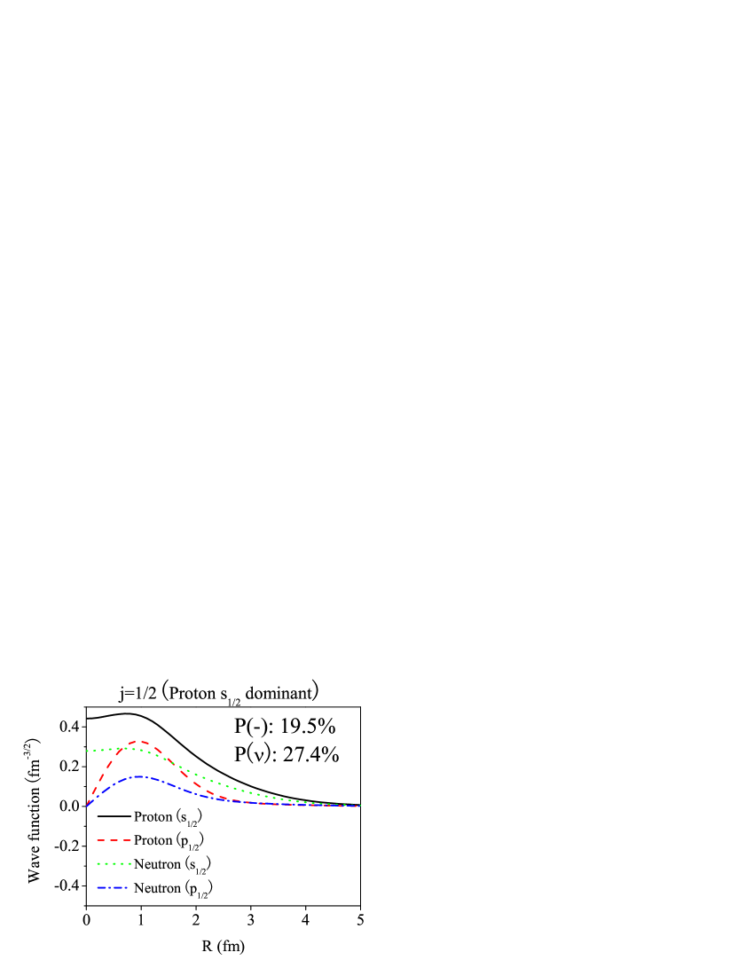
Figure 1: (Color online) Intrinsic single-particle wave function of the $j=1/2$ state with an $s_{1/2}$ proton component as a dominant one in ¹⁶O as a function of the radial distance $R$. The solid, dashed, dotted and dashed-dotted curves correspond $s_{1/2}$ proton, $p_{1/2}$ proton, $s_{1/2}$ neutron, and $p_{1/2}$ neutron respectively. $P(-)$ and $P(\nu)$ are the mixing probabilities of the negative-party and the neutron components respectively.

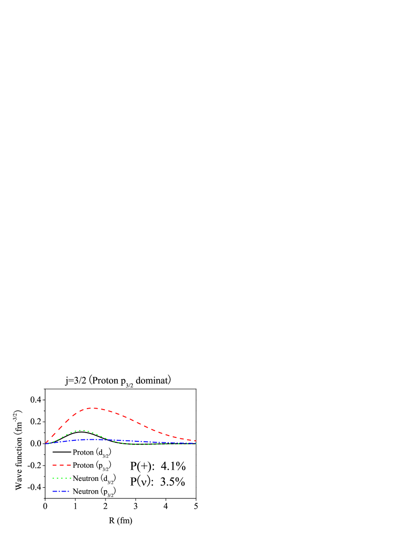
Figure 2: (Color online) Intrinsic single-particle wave function of the $j=3/2$ state with a $p_{3/2}$ proton component as a dominant one in ¹⁶O as a function of the radial distance $R$. The solid, dashed, dotted and dashed-dotted curves correspond $d_{3/2}$ proton, $p_{3/2}$ proton, $d_{3/2}$ neutron, and $p_{3/2}$ neutron respectively. $P(+)$ and $P(\nu)$ are the mixing probabilities of the positive-party and the neutron components respectively.

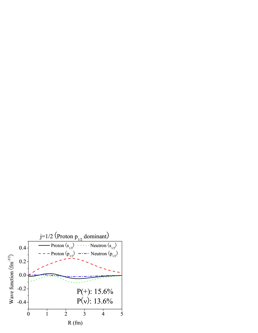
Figure 3: (Color online) Intrinsic single-particle wave function of the $j=1/2$ state with a $p_{1/2}$ proton component as a dominant one in ¹⁶O as a function of the radial distance $R$. The solid, dashed, dotted and dashed-dotted curves correspond $s_{1/2}$ proton, $p_{1/2}$ proton, $s_{1/2}$ neutron, and $p_{1/2}$ neutron respectively. $P(+)$ and $P(\nu)$ are the mixing probabilities of the positive-party and the neutron components respectively.

In Figs. 1, 2 and 3 the intrinsic single-particle wave functions in ¹⁶O with the strong tensor force ($x_{\text{T}}=1.5$) are plotted. The wave functions plotted have proton components as dominant ones. The wave function in Fig. 1 has a proton $s_{1/2}$ component as a dominant component. The mixing probabilities for negative parity ($p_{1/2}$) and neutron are 19.5% and 27.4% respectively. From the figure you can see that the spread of the $p_{1/2}$ components are smaller than the $s_{1/2}$ ones. It indicates that the opposite-parity components induced by the tensor force have high-momentum components. The wave function which has a proton $p_{3/2}$ component as a dominant one is plotted in Fig. 2 and the shrinkage of $d_{3/2}$ components compared to $p_{3/2}$ ones are clearly seen also. In the wave function which has a proton $p_{1/2}$ component as a dominant one, which is plotted in Fig. 3, the shrinkage is not so clear compared to the previous two cases, probably because of the orthogonality condition to the wave function to the first $j=1/2$ state in Fig. 1.

In the alpha particle case, $p_{1/2}$ components mixing into $s_{1/2}$ ones are also compact in size akaishi04 ; sugimoto04 ; ogawa06 . The importance of this shrinkage is confirmed in a shell model calculation myo05 and the antisymmetrized molecular dynamics (AMD) calculation dote05 , too. The present result infer that the shrinkage of mixing single-particle wave functions is generally important in heavier-mass region. There are also wave functions with a neutron component as a dominant one. The general tendency just mentioned above is almost the same if proton and neutron are interchanged.

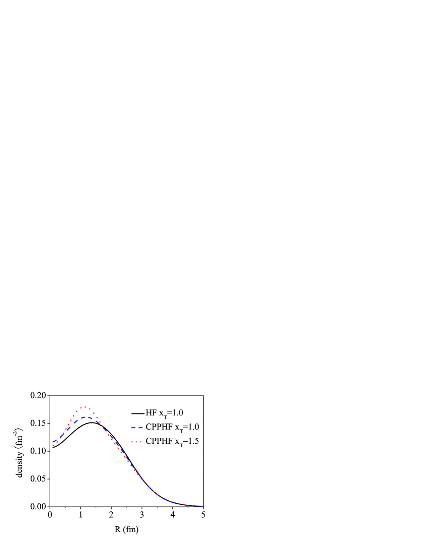
Figure 4: (Color online) Densities for ¹⁶O in the Hartree-Fock (HF) and the charge- and parity-projected Hartree-Fock (CPPHF) methods as a function of the radial distance ($R$). The solid, the dashed, and the dotted curves correspond to the HF calculation, the CPPHF calculation with the normal tensor force ($x_{\text{T}}=1.0$), and the CPPHF calculation with the strong tensor force ($x_{\text{T}}=1.5$).

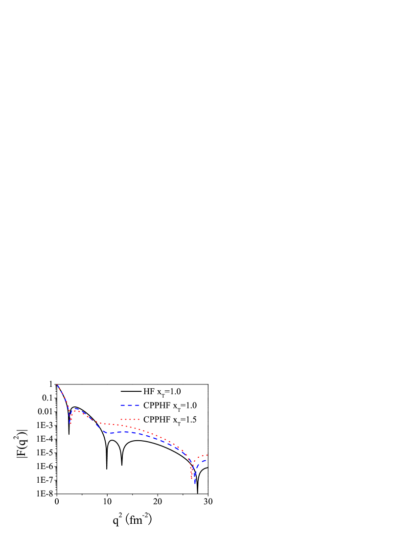
Figure 5: (Color online) Absolute values of the charge form factor for ¹⁶O in the Hartree-Fock (HF) and the charge- and parity-projected Hartree-Fock (CPPHF) methods as a function of the momentum squared ($q^{2}$). The solid, the dashed, and the dotted curves correspond to the HF calculation, the CPPHF calculation with the normal tensor force ($x_{\text{T}}=1.0$), and the CPPHF calculation with the strong tensor force ($x_{\text{T}}=1.5$).

In Fig. 4 the densities for ¹⁶O in the HF and CPPHF calculations are shown. Because the tensor force induces the opposite-parity components with narrower widths in single-particle wave functions, the densities are depleted in the middle in the CPPHF calculations compared to the one in the HF calculation. This effect is larger for the case with the strong tensor force as expected. To see the effect of the tensor correlation more clearly, in Fig. 5 the charge form factors are plotted as a function of the momentum squared. From the figure, higher-momentum components appear in the CPPHF calculation. It indicates that the tensor force enhances the charge form factor in a high-momentum region. The short-range correlation, which is not treated properly here, should have a contribution to the charge form factor in the high-momentum region. Hence, we need further investigation to compare the present result of the charge form factor in the CPPHF method with the experimental data. The enhancement of the charge form factor in a high-momentum region is also found in ⁴He in the calculation with the charge- and parity-projected relativistic mean field model ogawa06 .

III.2 Results for the oxygen isotopes

In this subsection we show the results for the sub-closed-shell oxygen isotopes.

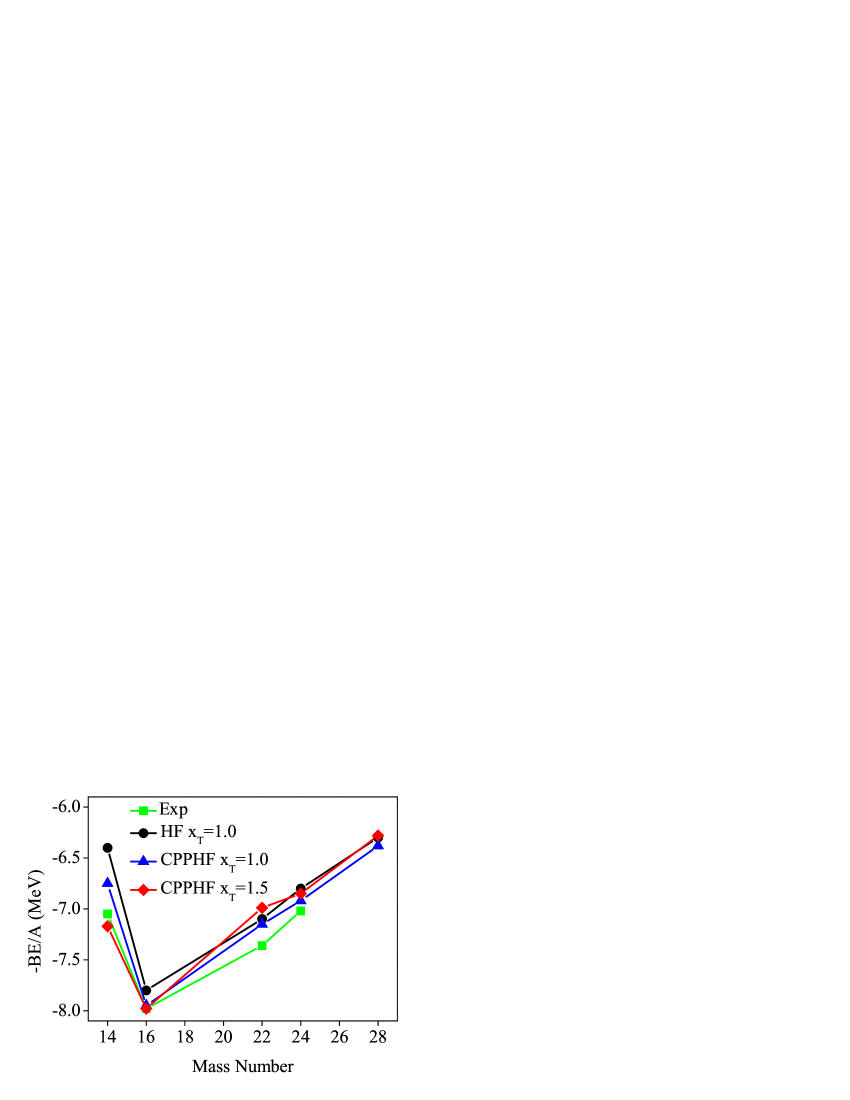
Figure 6: (Color online) Binding energies per particle with minus sign for sub-closed-shell oxygen isotopes. The horizontal line indicates mass numbers. The circle symbols correspond to the Hartree-Fock (HF) calculation, the triangle ones to the charge- and parity projected Hartree-Fock (CPPHF) calculation with the normal tensor force ($x_{\text{T}}=1.0$), and the diamond ones to the CPPHF calculation with the strong tensor force ($x_{\text{T}}=1.5$). The square symbols indicate the experimental data audi03 .

In Fig. 6, the results for the binding energies per particle in the Hartree-Fock (HF) calculation (the circle symbols), the charge- and parity-projected Hartree-Fock (CPPHF) calculation with the normal tensor force ($x_{\text{T}}$=1.0) (the triangle symbols) and the CPPHF calculation with the strong tensor force ($x_{\text{T}}$=1.5) (the diamond symbols) are shown. The experimental data (the square symbols) audi03 are also plotted.The general tendency is reproduced in our result, although the agreement with the experimental data is not as good as the Hartree-Fock-type calculations patyk99 ; bender03 ; vretenar05 ; nakada02 ; nakada06 . The HF calculation with the MV1 force underestimates the binding energy of ¹⁴O and ²²O a little bit largely. It indicates that if we adopt our calculation on the central and the density-dependent forces in the recent sophisticated effective interaction, the agreement with the experimental results should become better. There is an ambiguity in the treatment of the density-dependent force when we perform the parity and charge projections, because the density-dependent force cannot be written in a simple two-body operator form. It causes a difficulty when we use the density-dependent force in the CPPHF calculation. The optimization of the central force and the management of the density-dependent force will be our future problems. The agreement with the experimental data is good for ¹⁴O in the CPPHF method with the strong tensor force. In this case quite a large attractive potential energy comes from the tensor force as shown below.

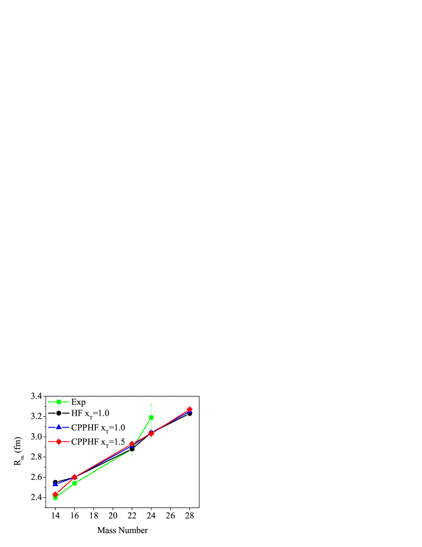
Figure 7: (Color online) Root-mean-square matter radii for sub-closed-shell oxygen isotopes. The horizontal line indicates mass numbers. The circle symbols correspond to the Hartree-Fock (HF) calculation, the triangle ones to the charge- and parity projected Hartree-Fock (CPPHF) calculation with the normal tensor force ($x_{\text{T}}=1.0$), and the diamond ones to the CPPHF calculation with the strong tensor force ($x_{\text{T}}=1.5$). The square symbols indicate the experimental data with error bars ozawa01 .

In Fig. 7, the results for the root-mean-square matter radii ($R_{\text{m}}$) are plotted with the experimental data ozawa01 . We use the same symbol for each case in Fig. 6. Except for ¹⁴O the results for all the three cases are almost the same and reproduce the experimental data well. For ¹⁴O the CPPHF calculation with the strong tensor force gives a smaller matter radius compared to the other two calculations and the agreement with the experimental data becomes better in the strong tensor force case. The reduction of the radius is caused by the shrinkage of the opposite parity component in a single-particle wave function induced by the tensor correlation. Such an effect cannot be treated in simple Hartree-Fock calculations.

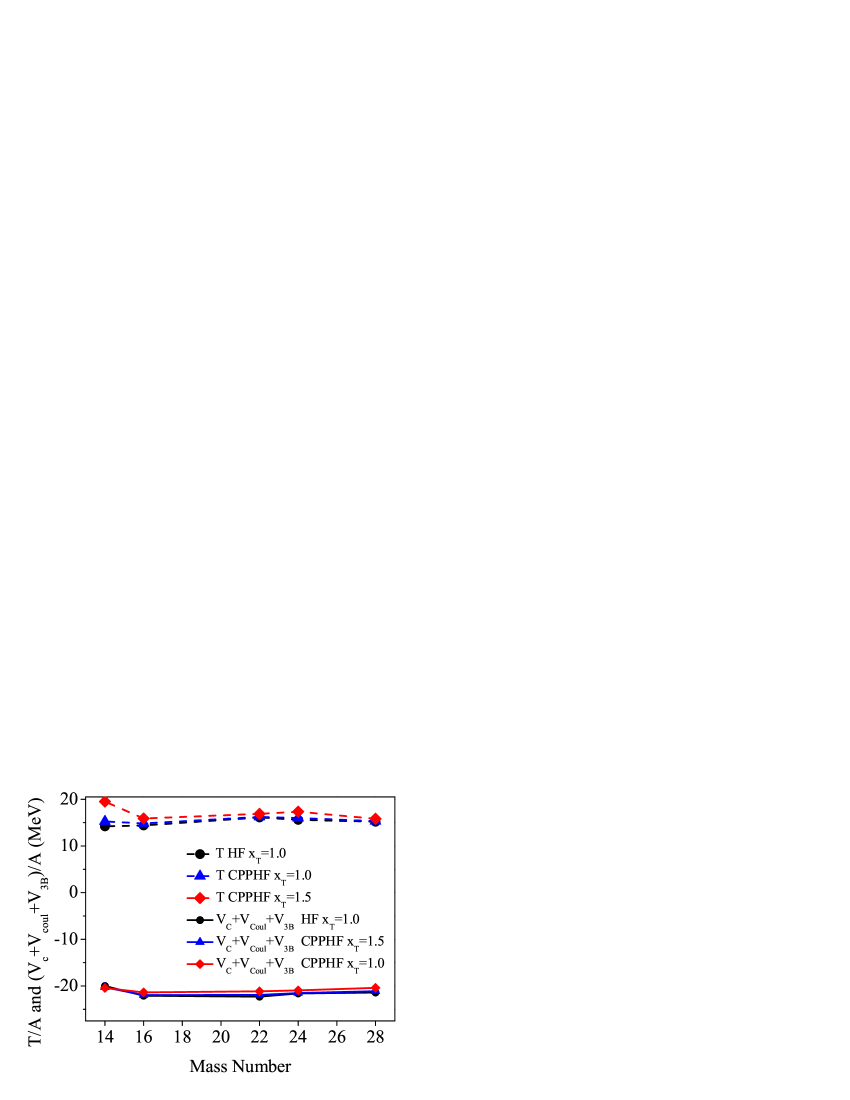
Figure 8: (Color online) Kinetic energy ($T$) per particle and the sum of the potential energies from the central force $V_{\text{C}}$, the Coulomb force $V_{\text{Coul}}$, and the three-body force $V_{\text{3B}}$ divided by mass numbers. The horizontal axis indicates mass numbers. The dashed lines correspond to the kinetic energy and the solid lines to the sum of the potential energies. The circle, triangle, and diamond symbols correspond to the Hartree-Fock (HF) calculation, the charge- and parity-projected Hartree-Fock (CPPHF) calculation with the normal tensor force ($x_{\text{T}}=1.0$), and the CPPHF calculation with the strong tensor force ($x_{\text{T}}=1.5$).

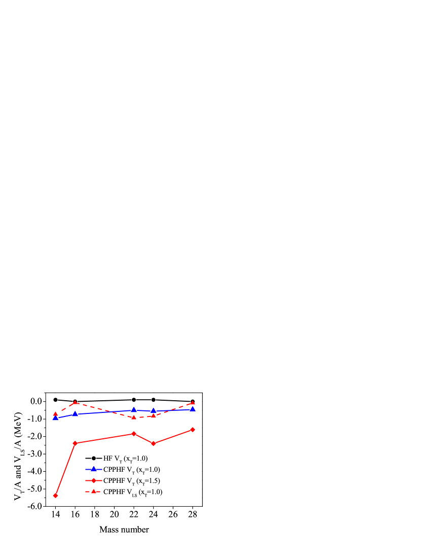
Figure 9: (Color online) Potential energies from the tensor force ($V_{\text{T}}$) and the LS force ($V_{\text{LS}}$) divided by mass numbers. The horizontal axis indicates mass numbers. The solid lines correspond to the potential energy from the tensor force. The dashed line corresponds to the potential energy from the LS force in the CPPHF calculation with the normal tensor force. Other results for the LS force are almost unchanged. The meanings of the symbols are the same as in Fig. 8.

To see the effect of the tensor force on the binding mechanism in the oxygen isotopes in Fig. 8 the results for the total kinetic energy $T$ (the dashed lines) and the sum of the potential energies from the central, the three-body and the Coulomb forces $V_{\text{C}}+V_{\text{3B}}+V_{\text{Coul}}$ (the solid lines) are plotted. We also show in Fig. 9 the result for the potential energies from the tensor force $V_{\text{T}}$ (the solid lines) and the LS force $V_{\text{LS}}$ (the dashed line). The same symbols are used for the HF calculation and the CPPHF calculations with the normal and strong tensor forces as in Fig. 6. All values are divided by mass numbers to make a isotope dependence clear. The total kinetic energy and the sum of the potential energies from the central, three-body and Coulomb forces show a volume-like behavior. The kinetic energy for ¹⁴O in the CPPHF calculation with the strong tensor force is larger than the other two cases. The increase of the kinetic energy is also caused by the strong tensor correlation in ¹⁴O, because to gain the correlation energy from the tensor force the opposite-parity components must mix into single-particle states and the opposite-parity components have larger kinetic energy.

The potential energies from the LS force behave in almost the same manner for the three cases. It becomes attractive if neutron shells are jj-closed and negligibly small if neutron shells are LS-closed. The potential energy from the tensor force becomes weakly repulsive in the HF calculation for all the oxygen isotopes. In the CPPHF calculations the potential energies from the tensor force become attractive for all the oxygen isotopes. In contrast to the LS potential energies, the tensor potential energies have sizable values in LS-closed shell nuclei like ¹⁶O and ²⁸O. The attraction from the tensor force is the same order that from the LS force even in the case with the normal tensor force. In CPPHF case $V_{\text{T}}$ becomes maximum in ¹⁴O and decreases with the mass number. For the strong tensor force case, the attractive energy from the tensor force becomes larger as expected. The attractive energy is quite large for ¹⁴O in the CPPHF calculation with the strong tensor force. For other isotopes the attractive energies from the tensor force are small and do not change so much with the mass number.

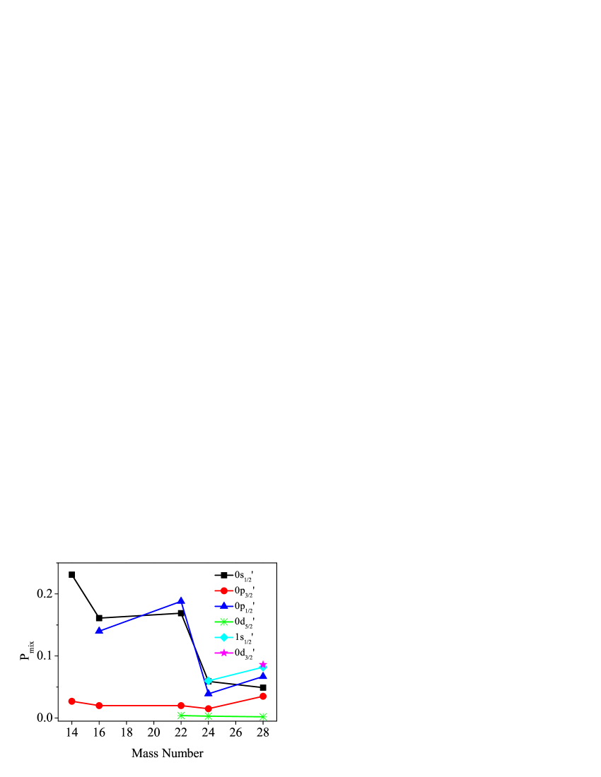
Figure 10: Probabilities of the mixing of the opposite parity components for single-particle states with neutron components as dominant ones in the charge- and parity projected Hartree-Fock calculation with the normal tensor force. The horizontal axis indicates mass numbers. The square, circle, triangle, asterisk, diamond, and star symbols correspond to the first $j$=1/2 ($0s_{1/2}^{\prime}$; $s_{1/2}$ dominant), the first $j$=3/2 (0$p_{3/2}^{\prime}$; $p_{3/2}$ dominant), the second $j$=1/2 ($0p_{1/2}^{\prime}$; $p_{1/2}$ dominant), the first $j$=5/2 ($0d_{5/2}^{\prime}$; $d_{5/2}$ dominant), the third $j$=1/2 ($1s_{1/2}^{\prime}$; $s_{1/2}$ dominant), and the second $j$=3/2 ($0d_{3/2}^{\prime}$; $d_{3/2}$ dominant), respectively.

In Fig. 10 the probabilities of the mixing of the opposite parity components $P_{\text{mix}}$ in the single-particle states with neutron components as the dominant ones in the result of the CPPHF calculation with the normal tensor force are shown. The result for the strong tensor case shows almost the same tendency. In the usual shell-model classification the first $j$=1/2 state ($s_{1/2}$ dominant), the first $j$=3/2 state ($p_{3/2}$ dominant), the second $j$=1/2 state ($p_{1/2}$ dominant), the first $j$=5/2 state ($d_{5/2}$ dominant), the third $j$=1/2 state ($s_{1/2}$ dominant), and the second $j$=3/2 state ($d_{3/2}$ dominant) correspond to $0s_{1/2}$, $0p_{3/2}$, $0p_{1/2}$, $0d_{5/2}$, $1s_{1/2}$, and $0d_{3/2}$ respectively. All those states are mixed states of positive and negative parities as in Eq. (32). We add a prime in the following to indicate each single-particle state has both positive-parity and negative-parity components. For example, a $0s_{1/2}^{\prime}$ state has $s_{1/2}$ (positive-parity) and $p_{1/2}$ (negative parity) components with an $s_{1/2}$ component as a dominant one. For ¹⁴O the neutron orbits are filled up to $0p_{3/2}^{\prime}$. The mixing probability of the opposite parity components for $0s_{1/2}^{\prime}$ is larger than 20% and that for $0p_{3/2}^{\prime}$ is a few % in ¹⁴O. In the CPPHF method the tensor correlation energy is gained by parity mixing and, therefore, $P_{\text{mix}}$ is a measure to indicate how each single-particle orbit contributes to the tensor correlation. The large $P_{\text{mix}}$ for $0s_{1/2}^{\prime}$ indicates that this orbit is largely affected by the tensor correlation. In ¹⁶O, the $0p_{1/2}^{\prime}$ neutron orbit is added newly. The addition of the $0p_{1/2}^{\prime}$ orbit reduces the parity mixing of the $0s_{1/2}^{\prime}$ because they have the same total angular momentum $j$=1/2. As the result, the tensor correlation energy becomes smaller. This effect is more significant for the strong tensor force case as seen in Fig. 9. In ²²O the neutron $0d_{5/2}^{\prime}$ is filled. Because there are no $j$=5/2 below, $P_{\text{mix}}$’s for the states filled already in ¹⁶O do not change largely. In ²⁴O the $1s_{1/2}^{\prime}$ orbit is newly occupied. The occupation of $1s_{1/2}^{\prime}$ reduces $P_{\text{mix}}$’s for the states with $j$=1/2, $0s_{1/2}^{\prime}$ and $0p_{1/2}^{\prime}$. The tensor correlation energy is enhanced, although the amount of the change is small. Finally, in ²⁸O the neutron $0d_{3/2}^{\prime}$ is filled. $P_{\text{mix}}$’s for the previously filled orbits change by this addition but the changes are not so large.

The change of $P_{\text{mix}}$ as shown above indicates that the large change of the tensor correlation energy from ¹⁴O to ¹⁶O in the strong tensor force case is caused by the blocking effect for the $j$=1/2 orbits. The blocking effect of this kind is shown to be important in the single-particle $ls$-splitting in ⁵He myo05 . The effect of the blocking is less significant for the excess neutron orbits. The effect of the blocking on binding energies in neutron excess oxygen isotopes seems to be small but the blocking may affect single-particle natures or collectivity in neutron excess oxygen isotopes, because the mixing probability is affected by the blocking effect.

The negligible $P_{\text{mix}}$ for the $0d_{5/2}^{\prime}$ orbit indicates that this orbit does not contribute to the tensor correlation although there is no other occupied orbits which have $j$=5/2. The main part of the tensor correlation comes from the $T=0$ channel. Because the proton $j$=5/2 orbit is not filled in neutron-excess oxygen isotopes, the $0d_{5/2}^{\prime}$ orbit is hard to contribute to the tensor correlation and the mixing probability of it becomes small.

IV Summary

We have studied the effect of the tensor force in the sub-closed-shell oxygen isotopes using the charge- and parity-projected Hartree-Fock (CPPHF) method. We have extended the CPPHF method to the cases with Hamiltonians including three-body forces, although the extension is straightforward. In the CPPHF method the parity and charge-number projections are performed before variation. By applying the CPPHF method to the oxygen isotopes actually, we have found that a sizable potential energy from the tensor force is obtained in the CPPHF method while in the Hartree-Fock calculation quite a small potential energy from the tensor force is obtained.

We have investigated ¹⁶O in some details. The correlation energy from the tensor force is about 10 MeV for the normal tensor force case and about 40 MeV for the strong tensor force case. In the strong tensor force case the strength of the $\tau_{1}\cdot\tau_{2}$ channel in the tensor force is multiplied by 1.5. The opposite parity components induced in single-particle states by the tensor force have compact sizes as compared to the normal parity components. This indicates that for the tensor correlation high-momentum components are important as already found in the alpha particle case akaishi04 ; sugimoto04 ; myo05 ; dote05 ; ogawa06 . The present result infers that the importance of the high-momentum component for the tensor correlation is valid in heavier mass nuclei. We have also shown the density and the charge form factor calculated in the CPPHF method. The density in the CPPHF method is reduced around the center and is pulled in to the inside region. This is caused by the parity mixing and the shrinkage of single-particle wave functions of opposite parities. The effect of the shrinkage appears in the charge form factor as a tail in a high-momentum region, because the shrinkage of the single-particle wave functions induces high-momentum components in the density.

In the results for the oxygen isotopes, the general tendencies for the binding energies and the matter radii are reproduced in the CPPHF calculation with the effective interaction adopted here, while the agreement of the binding energy with the experimental data is not so good compared to the Hartree-Fock-type calculations with recent effective interactions. The root-mean-square matter radii are well reproduced within error bars except for ¹⁴O with both the normal tensor force and the strong tensor force. In the strong tensor force case, the matter radius of ¹⁴O becomes smaller and close to the experimental data. The reduction of the matter radius in ¹⁴O with the strong tensor force is due to the shrinkage of single-particle wave function by the strong tensor correlation, which is large in ¹⁴O. Because the $0p_{1/2}$ neutron orbit is not occupied in ¹⁴O, there are no blocking states for the $0s_{1/2}$ proton orbit in the tensor correlation and, therefore, the tensor correlation becomes large. Actually, the correlation energy from the tensor force per particle amounts to more than 5 MeV in this case. For all the oxygen isotopes the calculated potential energy from the tensor force is in the same order as that from the LS force for the normal tensor force case. In the strong tensor force case it becomes about two times larger. In contrast to the potential energy from the LS force, the potential energy from the tensor force in an LS-closed-shell nucleus does not become close to zero in the CPPHF calculation. In the Hartree-Fock calculation it becomes negligibly small because both the total spin and the total orbital angular momenta is almost zero in an LS-closed-shell nucleus. The sudden decrease of the potential energy from the tensor force from ¹⁴O to ¹⁶O is attributed to the blocking effect of the $j$=1/2 orbits. The blocking effect is also seen in the neutron-excess oxygen isotopes but does not affect the binding energy largely.

In the present study we have applied the CPPHF method to the ground states of the sub-closed-shell oxygen isotopes. The application to odd-mass nuclei and open-shell nuclei to study the effect of the tensor force on single-particle natures and the change of collectivity by the tensor correlation in a neutron excess region are interesting because the tensor force changes the spin, the orbital angular momenta and the isospin of nucleon orbits simultaneously, which is realized in the CPPHF method by the parity and charge mixing. As for an effective interaction, we combine the available effective interaction and the tensor force in the free space with some modifications. We need to use effective interactions which have the connection with the realistic nuclear forces to reveal the relation between nuclear structure and the underlying nuclear force and have the consistency between the tensor force and other forces like the central and LS forces. The study in such a direction is also important and now under progress.

References

• (1) H.A. Bethe, Annu. Rev. Nucl. Sci. 21, 93 (1971).
• (2) Y. Akaishi, in Cluster Models and Other Topics, edited by T.T.S. Kuo and E. Osnes (World Scientific, Singapore, 1986), p. 259.
• (3) H. Kamada, A. Nogga, W. Glöckle, E. Hiyama, M. Kamimura, K. Varga, Y. Suzuki, M. Viviani, A. Kievsky, S. Rosati, J. Carlson, S.C. Pieper, R.B. Wiringa, P. Navrátil, B.R. Barrett, N. Barnea, W. Leidemann, and G. Orlandini, Phys. Rev. C 64, 044001 (2001).
• (4) S. Takagi, W. Watari, and M. Yasuno, Prog. Theor. Phys. 22, 549 (1959); T. Terasawa, Prog. Theor. Phys. 23, 87 (1960); A. Arima and T. Terasawa, Prog. Theor. Phys. 23, 115 (1960).
• (5) K. Andō and H. Bandō, Prog. Theor. Phys. 66, 227 (1980).
• (6) T. Myo, K. Katō, and K. Ikeda, Prog. Theor. Phys. 113, 763 (2005).
• (7) A. Ozawa, T. Kobayashi, T. Suzuki3, K. Yoshida, and I. Tanihata, Phys. Rev. Lett. 84, 5493 (2000).
• (8) H. Grawe, Springer Lect. Notes in Phys. 651, 33 (2004).
• (9) T. Otsuka, T. Suzuki, R. Fujimoto, H. Grawe, and Y. Akaishi Phys. Rev. Lett. 95, 232502 (2005)
• (10) H. Toki, S. Sugimoto, and K. Ikeda, Prog. Theor. Phys. 108 903 (2002).
• (11) Y. Ogawa, H. Toki, S. Tamenaga, H. Shen, A. Hosaka, S. Sugimoto, and K. Ikeda, Prog. Theor. Phys. 111, 75 (2004).
• (12) S. Sugimoto, K. Ikeda, and H. Toki, Nucl. Phys. A 740, 77 (2004).
• (13) Y. Ogawa, H. Toki, S. Tamenaga, S. Sugimoto, and K. Ikeda, Phys. Rev C 73, 034301 (2006).
• (14) S. Sugimoto, K. Ikeda, and H. Toki, nucl-th/0511087.
• (15) Y. Akaishi, Nucl. Phys. A 738, 80 (2004).
• (16) A. Doté, Y. Kanada-En’yo, H. Horiuchi, Y. Akaishi, K. Ikeda, Prog. Theor. Phys. 115, 1069 (2006).
• (17) T. Neff and H. Feldmeier, Nucl. Phys. A 713, 311 (2004).
• (18) R. Roth, P. Papakonstantinou, N. Paar, H. Hergert, T. Neff, and H. Feldmeier, Phys. Rev. C 73, 044312 (2006).
• (19) R.M. Tarbutton and K.T.R. Davies, Nucl Phys. A 120,1 (1968).
• (20) A. Bouyssy, J.-F. Mathiot, N. Van Giai, and S. Marcos, Phys. Rev. C 36, 380 (1987).
• (21) T. Ando, K. Ikeda, and A. Tohsaki-Suzuki, Prog. Theor. Phys. 64, 1608 (1980).
• (22) A. B. Volkov, Nucl. Phys. 74, 33 (1965).
• (23) R. Tamagaki, Prog. Theor. Phys. 39, 91 (1968).
• (24) D. Vautherin and D.M. Brink, Phys. Rev. C 5 626 (1972).
• (25) Z. Patyk, A. Baran, J.F. Berger, J. Dechargé J. Dobaczewski, P. Ring, and A. Sobiczewski, Phys. Rev. C 59, 704 (1999).
• (26) T. Myo et al. in preparation.
• (27) P.-G. Reinhard, in Cmpulationl Nuclear Phyiscs 1 (edited by K. Langanke, J.A. Maruhn, and S.E. Koonin, Springer-Verlag, Berlin, 1991) Chapter 2.
• (28) H. Flocard, P. Quentin, A.K. Kerman, and D. Vautherin, Nucl. Phys. A 203, 433 (1973).
• (29) G. Audi, A. H. Wapstra and C. Thibault, Nucl. Phys. A 729, 337 (2003).
• (30) A. Ozawa, T. Suzuki and I. Tanihata, Nucl. Phys. A 693, 32 (2001).
• (31) M. Bender, P.-H. Heenen, and P.-G. Reinhard, Rev. Mod. Phys. 75, 121 (2003) and the references therein.
• (32) D. Vretenar, A.V. Afanasjev, G.A. Lalazissis, and P. Ring, Phys. Rep. 409, 101 (2005) and the references therein.
• (33) H. Nakada and M. Sato, Nucl. Phys. A 699, 511 (2002).
• (34) H. Nakada, Nucl. Phys. A 764, 117 (2006).