E-mail address: ] dang@riken.jp

Consistency of particle-particle random-phase approximation
and its renormalizations111to appear in Physical Review C

Nguyen Dinh Dang [ 1) Heavy-ion nuclear physics laboratory, Nishina Center for Accelerator-Based Science, RIKEN, 2-1 Hirosawa, Wako city, 351-0198 Saitama, Japan
2) Institute for Nuclear Science and Technique, Hanoi, Vietnam
Abstract

The consistency condition is tested within the particle-particle random-phase approximation (RPA), renormalized RPA (RRPA) and the self-consistent RPA (SCRPA) making use of the Richardson model of pairing. The two-particle separation energy is calculated in two ways, namely as the energy of the first addition mode, which adds two particles to a core with $N$ particles, and as the energy of the first removal mode, which removes two particles from the $N+2$ particle system to get back to the same $N$-particle core. The corresponding transitions generated by the pairing operators are also calculated. It is found that the results obtained in these two ways of calculations are close to each other only at large values of particle number $N$ and/or small interaction strength. At $N\leq$ 10 for a given value of the interaction strength, the discrepancy between the results obtained in two ways of calculations within the SCRPA is much smaller than those given by the RPA and RRPA.

pacs:
21.60.Jz, 21.60.-n, 21.10.Dr

I Introduction

The random-phase approximation (RPA) has been widely used in the theoretical study of nuclei within the valley of $\beta$-stability. The success of the RPA is mainly based on the use of the quasiboson approximation (QBA), which considers fermion pairs as boson operators, just neglecting the Pauli principle between them. As a result, a set of linear equations, called the RPA equations, was derived, which reveals the physics of collective excitations generated by the RPA boson-like modes. The simplicity of the RPA equations allows a feasible treatment of a number of many-body problems, which would be computationally intractable otherwise. However, this approach suffers a drawback: It breaks down at a certain critical value of the interaction’s parameter, where the RPA yields imaginary solutions. The reason of this well-known RPA instability is the violation of Pauli principle within the QBA.

In $\beta$-stable medium and heavy nuclei, the QBA is a good approximation, and the RPA is a very powerful tool for the description of several important quantities such as the ground-state and excited-state energies, electro-magnetic transition probabilities and their distribution, transition densities, etc. The first-order diagram expansion beyond the mean field treated within the RPA includes significant effects of two-body correlations beyond the mean-field. However, with reducing the particle number, the concept of collective excitations, which are described by the RPA modes, becomes less and less firm. The ground-state correlations (GSC) which are left beyond the RPA become stronger in light systems. This feature makes the validity of the QBA, and therefore of the RPA itself, questionable in the systems with small particle numbers.

Several approaches were developed to take into account the GSC beyond RPA in a simple way such as to restore the Pauli principle among the fermion pairs, from which the RPA operators are constructed. The popular one, known as the renormalized RPA (RRPA)Β Hara (1, 2, 3, 4), includes the expectation value over the ground state of the diagonal elements of the commutator between two fermion-pair operators, neglected in the QBA. In this way the Pauli principle is approximately taken care of. The inclusion of GSC beyond RPA within the RRPA eventually renormalizes the interaction in such a way that the collapse of RPA is avoided, and the RRPA has solutions at any value of the interaction’s parameter. This scheme has been tested in several exactly solvable schematic models such as the Lipkin model for $ph$ RRPAΒ Hara (1, 4), the SO(8) model for the renormalized quasiparticle RPAΒ RQRPA (5), and the Richardson model for the $pp$ RRPA and self-consistent RPA (SCRPA)Β Duk (6, 7). The results of these studies showed that the difference between the energies of the first excited state given by the $pp$ RPA, $pp$ RRPA, and SCRPA increases noticeably with increasing the interaction parameter and/or decreasing the particle number. The SCRPA solutions are the closest ones to the exact solutions. These results raise a serious question of the applicability of the RPA to the calculations for realistic light-neutron rich nuclei. As a matter of fact, a close agreement between the RPA results and the experimental data for light neutron-rich nuclei can be considered really reasonable if the corrections due to GSC beyond RPA are negligible, which justify the validity of the QBAΒ VinhMau (8). In the opposite case such agreement may be even illusory.

This concern is the motivation of the present work, whose goal is to test the consistency of the $pp$ RPA and its renormalizations, the $pp$ RRPA and SCRPA, at different particle numbers as the interaction strength varies. The reason of choosing the $pp$ RPA comes from one of its major merits, which allows the straightforward calculation of an important quantity in the study of unstable nuclei, namely the two-particle separation energy. Indeed, the $pp$ RPA uses the addition and removal phonon operators to create the ground states and excited states of the systems with $N+2$ and $N-2$ particles, respectively, from the ground state of the $N$-particle system. Therefore the two-particle separation energy of the $(N+2)$-particle system can be calculated either as the energy of the lowest excited state generated by the addition mode, which adds two particles to the core with N particles, or as that generated by the removal mode, which removes two particles from the core with $N+2$ particles. A consistent theory should give identical results in either way of calculation. By analyzing the results obtained in two ways of calculations within all three approaches, namely the RPA, RRPA, and SCRPA in their application to an exactly solvable schematic model, namely the Richardson modelΒ Ric (9), the present work may shed light on the consistency of these approaches, in particular, in their application to systems with small particle numbers (light systems).

The paper is organized as follows. The brief outline of the $pp$ RPA, RRPA, and SCRPA applied to the Richardson model is presented in Sec. II. As the present paper deals only with $pp$ RPA and its renormalization, the prefix $pp$ will be omitted hereafter. The results of numerical calculations are analyzed in Sec. III. The paper is summarized in the last section, where conclusions are drawn.

II RPA, RRPA and SCRPA within the Richardson model

II.1 The Richardson model

The Richardson model, considered in the present paper, consists of $\Omega$ doubly-fold equidistant levels, which interact via a pairing force with parameter $G$. The model Hamiltonian is given as  Duk (6, 7)

$$H=\sum_{i=1}^{\Omega}(\epsilon_{i}-\lambda)N_{i}-G\sum_{i,j=1}^{\Omega}P_{i}^{\dagger}P_{j}~{},$$ (1)

where the particle-number operator $N_{i}$ and pairing operators $P_{i}^{\dagger}$, $P_{i}$ are defined as

$$N_{i}=c_{i}^{\dagger}c_{i}+c_{-i}^{\dagger}c_{-i}~{},\hskip 14.22636ptP_{i}^{\dagger}=c_{i}^{\dagger}c_{-i}^{\dagger}~{},\hskip 14.22636ptP_{i}=(P_{i}^{\dagger})^{\dagger}~{}.$$ (2)

These operators fulfill the following exact commutation relations

$$[P_{i},P_{j}^{\dagger}]=\delta_{ij}(1-N_{i})~{},$$ (3)
$$[N_{i},P_{j}^{\dagger}]=2\delta_{ij}P_{j}^{\dagger},~{}\hskip 14.22636pt[N_{i},P_{j}]=-2\delta_{ij}P_{j}~{}.$$ (4)

The single-particle energies of the equidistant levels are defined as $\epsilon_{i}=i\epsilon$ with $i$ running over all $\Omega$ levels. The present paper considers only the $ph$-symmetric case. This means that, in the absence of interaction ($G=$0), the lowest $\Omega/2$ levels are filled with $N=\Omega$ particles (two particles on each level). Numerating particle ($p$) and hole ($h$) levels from the levels nearest to the Fermi level, the particle and hole energies are equal to $\epsilon_{p}=\epsilon(\Omega/2+p)$ and $\epsilon_{h}=\epsilon(\Omega/2-h+1)$, respectively, with $p$ ($h$) $=$ 1, …, $\Omega/2$. The Fermi level $\epsilon_{\rm F}$ is defined as

$$\epsilon_{\rm F}=[\epsilon(\Omega+1)-{G}]/2~{}.$$ (5)

There are several methods of solving exactly the pairing problem described by Hamiltonian (1), namely the Richardson methodΒ Ric (9), the infinite-dimensional algebras in Ref. Pan (10), and the direct diagonalization of Hamiltonian (1) in the Fock spaceΒ Volya (11).

II.2 RPA

The outline of the RPA is given in detail in Ref. Ring (12). It uses the addition Aμ†subscriptsuperscriptπ΄β€ πœ‡A^{\dagger}_{\mu} and removal Rλ†subscriptsuperscriptπ‘…β€ πœ†R^{\dagger}_{\lambda} phonon operators to create the ground states and excited states of the systems with $N+2$ and $N-2$ particles, respectively, from the ground state of the $N$-particle system. Applied to the Richardson model, these addition and removal phonon operators are given as

Aμ†=βˆ‘pXp(ΞΌ)​Qpβ€ βˆ’βˆ‘hYh(ΞΌ)​Qh,superscriptsubscriptπ΄πœ‡β€ subscript𝑝superscriptsubscriptπ‘‹π‘πœ‡subscriptsuperscript𝑄†𝑝subscriptβ„Žsuperscriptsubscriptπ‘Œβ„Žπœ‡subscriptπ‘„β„Ž{A}_{\mu}^{\dagger}=\sum_{p}X_{p}^{(\mu)}Q^{\dagger}_{p}-\sum_{h}Y_{h}^{(\mu)}Q_{h}~{}, (6)

and

Rλ†=βˆ‘hXh(Ξ»)​Qhβ€ βˆ’βˆ‘pYp(Ξ»)​Qp,superscriptsubscriptπ‘…πœ†β€ subscriptβ„Žsuperscriptsubscriptπ‘‹β„Žπœ†subscriptsuperscriptπ‘„β€ β„Žsubscript𝑝superscriptsubscriptπ‘Œπ‘πœ†subscript𝑄𝑝{R}_{\lambda}^{\dagger}=\sum_{h}X_{h}^{(\lambda)}Q^{\dagger}_{h}-\sum_{p}Y_{p}^{(\lambda)}Q_{p}~{}, (7)

respectively, where

Qp†=Pp†,Qh=βˆ’Ph†.formulae-sequencesubscriptsuperscript𝑄†𝑝subscriptsuperscript𝑃†𝑝subscriptπ‘„β„Žsubscriptsuperscriptπ‘ƒβ€ β„ŽQ^{\dagger}_{p}=P^{\dagger}_{p}~{},\hskip 14.22636ptQ_{h}=-P^{\dagger}_{h}~{}. (8)

The RPA assumes the validity of the QBA, which replaces the expectation value of the commutation relations $[Q_{i},Q^{\dagger}_{j}]$ in the RPA ground state $|N,0\rangle$ of $N$-particle system with that obtained in the Hartree-Fock (HF) ground state $|{\rm HF}\rangle$, namely

$$\langle{N,0}|[{Q}_{i},{Q}_{j}^{\dagger}]|{N,0}\rangle\simeq\langle{\rm HF}|[{Q}_{i},{Q}_{j}^{\dagger}]|{\rm HF}\rangle=\delta_{ij}~{},\hskip 14.22636pt(i,j)=(p,p^{\prime})~{},(h,h^{\prime})~{},$$ (9)

since $\langle{\rm HF}|N_{p}|{\rm HF}\rangle=$ 0, and $\langle{\rm HF}|N_{h}|{\rm HF}\rangle=$ 2. Using the QBA (9), one can easily verify that the expectation values of the commutation relations for addition and removal operators in the RPA ground state are of bosonic type, i.e.

⟨N,0|[AΞΌ,Aμ′†]|N,0⟩=δμ​μ′,⟨N,0|[RΞ»,Rλ′†]|N,0⟩=δλ​λ′,formulae-sequencequantum-operator-product𝑁0subscriptπ΄πœ‡superscriptsubscript𝐴superscriptπœ‡β€²β€ π‘0subscriptπ›Ώπœ‡superscriptπœ‡β€²quantum-operator-product𝑁0subscriptπ‘…πœ†superscriptsubscript𝑅superscriptπœ†β€²β€ π‘0subscriptπ›Ώπœ†superscriptπœ†β€²\langle N,0|[A_{\mu},A_{\mu^{\prime}}^{\dagger}]|N,0\rangle=\delta_{\mu\mu^{\prime}}~{},\hskip 14.22636pt\langle N,0|[R_{\lambda},R_{\lambda^{\prime}}^{\dagger}]|N,0\rangle=\delta_{\lambda\lambda^{\prime}}~{}, (10)

if the $X$ and $Y$ amplitudes obey the following normalization (orthogonality) conditions

$$\sum_{p}X_{p}^{(\mu)}X_{p}^{(\mu^{\prime})}-\sum_{h}Y_{h}^{(\mu)}Y_{h}^{(\mu^{\prime})}=\delta_{\mu\mu^{\prime}}~{},\hskip 5.69054pt\sum_{h}X_{h}^{(\lambda)}X_{h}^{(\lambda^{\prime})}-\sum_{p}Y_{p}^{(\lambda)}Y_{p}^{(\lambda^{\prime})}=\delta_{\lambda\lambda^{\prime}}~{},$$
$$\sum_{p}X_{p}^{(\mu)}Y_{p}^{(\lambda)}-\sum_{h}X_{h}^{(\lambda)}Y_{h}^{(\mu)}=0~{},$$ (11)

while the closure relations

$$\sum_{\mu}X_{p}^{(\mu)}X_{p^{\prime}}^{(\mu)}-\sum_{\lambda}Y_{p}^{(\lambda)}Y_{p^{\prime}}^{(\lambda)}=\delta_{pp^{\prime}}~{},\hskip 5.69054pt\sum_{\lambda}X_{h}^{(\lambda)}X_{h^{\prime}}^{(\lambda)}-\sum_{\mu}Y_{h}^{(\mu)}Y_{h^{\prime}}^{(\mu)}=\delta_{hh^{\prime}}~{},$$
$$\sum_{\lambda}X_{h}^{(\lambda)}Y_{p}^{(\lambda)}-\sum_{\mu}X_{p}^{(\mu)}Y_{h}^{(\mu)}=0~{}$$ (12)

guarantee the following inverse transformation of Eqs. (6) and (7)

Qp†=[βˆ‘ΞΌXp(ΞΌ)​Aμ†+βˆ‘Ξ»Yp(Ξ»)​RΞ»],Qh=[βˆ‘Ξ»Xh(Ξ»)​RΞ»+βˆ‘ΞΌYh(ΞΌ)​Aμ†].formulae-sequencesuperscriptsubscript𝑄𝑝†delimited-[]subscriptπœ‡superscriptsubscriptπ‘‹π‘πœ‡superscriptsubscriptπ΄πœ‡β€ subscriptπœ†superscriptsubscriptπ‘Œπ‘πœ†subscriptπ‘…πœ†subscriptπ‘„β„Ždelimited-[]subscriptπœ†superscriptsubscriptπ‘‹β„Žπœ†subscriptπ‘…πœ†subscriptπœ‡superscriptsubscriptπ‘Œβ„Žπœ‡superscriptsubscriptπ΄πœ‡β€ Q_{p}^{\dagger}=\bigg{[}\sum_{\mu}X_{p}^{(\mu)}A_{\mu}^{\dagger}+\sum_{\lambda}Y_{p}^{(\lambda)}R_{\lambda}\bigg{]}~{},\hskip 14.22636ptQ_{h}=\bigg{[}\sum_{\lambda}X_{h}^{(\lambda)}R_{\lambda}+\sum_{\mu}Y_{h}^{(\mu)}A_{\mu}^{\dagger}\bigg{]}~{}. (13)

The RPA equations are obtained by linearizing the equation of motion with Hamiltonian (1) and operators $A^{\dagger}$ and $R^{\dagger}$. The matrix form of the RPA equation for the addition mode is

$$\left(\begin{array}[]{cc}{A}&{B}\\ -{B}&{C}\end{array}\right)\left(\begin{array}[]{c}{X^{(\mu)}}\\ {Y^{(\mu)}}\end{array}\right)=E_{\mu}\left(\begin{array}[]{c}{X^{(\mu)}}\\ {Y^{(\mu)}}\end{array}\right)~{},$$ (14)

where the submatrices $A$, $B$, and $C$ are found as Duk (6, 12)

$$A_{pp^{\prime}}^{\rm RPA}=\langle{\rm HF}|[{Q}_{p},[H,{Q}_{p^{\prime}}^{\dagger}]]|{\rm HF}\rangle=2\bigg{[}\epsilon\bigg{(}p-\frac{1}{2}\bigg{)}+\frac{G}{2}\bigg{]}\delta_{pp^{\prime}}-G~{},$$ (15)
$$B_{ph}^{\rm RPA}=-\langle{\rm HF}|[{Q}_{p},[H,{Q}_{h}]]|{\rm HF}\rangle=G~{},$$ (16)
Ch​hβ€²RPA=βˆ’βŸ¨HF|[Qh,[H,Qh′†]]|HF⟩=βˆ’2​[ϡ​(hβˆ’12)+G2]​δh​hβ€²+G.superscriptsubscriptπΆβ„Žsuperscriptβ„Žβ€²RPAquantum-operator-productHFsubscriptπ‘„β„Žπ»superscriptsubscript𝑄superscriptβ„Žβ€²β€ HF2delimited-[]italic-Ο΅β„Ž12𝐺2subscriptπ›Ώβ„Žsuperscriptβ„Žβ€²πΊC_{hh^{\prime}}^{\rm RPA}=-\langle{\rm HF}|[{Q}_{h},[H,{Q}_{h^{\prime}}^{\dagger}]]|{\rm HF}\rangle=-2\bigg{[}\epsilon\bigg{(}h-\frac{1}{2}\bigg{)}+\frac{G}{2}\bigg{]}\delta_{hh^{\prime}}+G~{}. (17)

II.3 RRPA

The QBA (9) neglects GSC beyond RPA. The latter make the expectation value of $N_{p}$ deviate from zero and that of $N_{h}$ deviate from 2. In order to take this effect into account, the RRPA considers the following renormalized addition and removal phonon operators

π’œΞΌβ€ =βˆ‘pXp(ΞΌ)​QΒ―pβ€ βˆ’βˆ‘hYh(ΞΌ)​QΒ―h,andℛλ†=βˆ‘hXh(Ξ»)​QΒ―hβ€ βˆ’βˆ‘pYp(Ξ»)​QΒ―p,formulae-sequencesuperscriptsubscriptπ’œπœ‡β€ subscript𝑝superscriptsubscriptπ‘‹π‘πœ‡superscriptsubscript¯𝑄𝑝†subscriptβ„Žsuperscriptsubscriptπ‘Œβ„Žπœ‡subscriptΒ―π‘„β„Žandsuperscriptsubscriptβ„›πœ†β€ subscriptβ„Žsuperscriptsubscriptπ‘‹β„Žπœ†superscriptsubscriptΒ―π‘„β„Žβ€ subscript𝑝superscriptsubscriptπ‘Œπ‘πœ†subscript¯𝑄𝑝{\cal A}_{\mu}^{\dagger}=\sum_{p}{{X}_{p}^{(\mu)}}\overline{Q}_{p}^{\dagger}-\sum_{h}{{Y}_{h}^{(\mu)}}\overline{Q}_{h}~{},\hskip 14.22636pt{\rm and}\hskip 14.22636pt{\cal R}_{\lambda}^{\dagger}=\sum_{h}{{X}_{h}^{(\lambda)}}\overline{Q}_{h}^{\dagger}-\sum_{p}{Y}_{p}^{(\lambda)}\overline{Q}_{p}~{}, (18)

respectivelyΒ , with the abbreviation

π’ͺΒ―i†=π’ͺiβ€ βŸ¨Di⟩,π’ͺΒ―i=π’ͺi⟨Di⟩,⟨DiβŸ©β‰‘βŸ¨N,0~|Di|N,0~⟩,i=p,h,formulae-sequencesuperscriptsubscriptΒ―π’ͺ𝑖†superscriptsubscriptπ’ͺ𝑖†delimited-⟨⟩subscript𝐷𝑖formulae-sequencesubscriptΒ―π’ͺ𝑖subscriptπ’ͺ𝑖delimited-⟨⟩subscript𝐷𝑖formulae-sequencedelimited-⟨⟩subscript𝐷𝑖quantum-operator-product~𝑁0subscript𝐷𝑖~𝑁0π‘–π‘β„Ž\overline{\cal O}_{i}^{\dagger}=\frac{{\cal O}_{i}^{\dagger}}{\sqrt{\langle D_{i}\rangle}}~{},\hskip 14.22636pt\overline{\cal O}_{i}=\frac{{\cal O}_{i}}{\sqrt{\langle D_{i}\rangle}}~{},\hskip 14.22636pt\langle D_{i}\rangle\equiv\langle\widetilde{N,0}|D_{i}|\widetilde{N,0}\rangle~{},\hskip 14.22636pti=p,~{}h~{}, (19)

where the correlated ground state $|\widetilde{N,0}\rangle$ is defined as the vacuum of the operators ${\cal A}_{\mu}$ and ${\cal R}_{\lambda}$, i.e.

$${\cal A}_{\mu}|\widetilde{N,0}\rangle={\cal R}_{\lambda}|\widetilde{N,0}\rangle=0~{}.$$ (20)

The GSC factors $\langle D_{i}\rangle$ are the expectation values of the operators

$$D_{p}=1-N_{p}~{},\hskip 14.22636ptD_{h}=N_{h}-1~{},$$ (21)

in the correlated ground state $|\widetilde{N,0}\rangle$ (20). They are introduced in the definition (18) to preserve the ground-state expectation value of the commutation relation (3). Indeed, using Eq. (3) and definition (8), one obtains the exact commutation relations for operators $Q_{i}$ and $Q^{\dagger}_{i}$ in the form

[Qp,Qp′†]=Ξ΄p​p′​Dp,[Qh,Qh′†]=Ξ΄h​h′​Dh.formulae-sequencesubscript𝑄𝑝superscriptsubscript𝑄superscript𝑝′†subscript𝛿𝑝superscript𝑝′subscript𝐷𝑝subscriptπ‘„β„Žsuperscriptsubscript𝑄superscriptβ„Žβ€²β€ subscriptπ›Ώβ„Žsuperscriptβ„Žβ€²subscriptπ·β„Ž[Q_{p},Q_{p^{\prime}}^{\dagger}]=\delta_{pp^{\prime}}D_{p}~{},\hskip 14.22636pt[Q_{h},Q_{h^{\prime}}^{\dagger}]=\delta_{hh^{\prime}}D_{h}~{}. (22)

Using this exact relation (22) and the definition (20), one can see that the renormalized addition and removal operators satisfy the boson commutation relations in the correlated ground state (20)

⟨[π’œΞΌ,π’œΞΌβ€²β€ ]⟩=δμ​μ′,⟨[β„›Ξ»,ℛλ′†]⟩=δλ​λ′,formulae-sequencedelimited-⟨⟩subscriptπ’œπœ‡superscriptsubscriptπ’œsuperscriptπœ‡β€²β€ subscriptπ›Ώπœ‡superscriptπœ‡β€²delimited-⟨⟩subscriptβ„›πœ†superscriptsubscriptβ„›superscriptπœ†β€²β€ subscriptπ›Ώπœ†superscriptπœ†β€²\langle[{\cal A}_{\mu},{\cal A}_{\mu^{\prime}}^{\dagger}]\rangle=\delta_{\mu\mu^{\prime}}~{},\hskip 14.22636pt\langle[{\cal R}_{\lambda},{\cal R}_{\lambda^{\prime}}^{\dagger}]\rangle=\delta_{\lambda\lambda^{\prime}}~{}, (23)

if the amplitudes ${X}$ and ${Y}$ satisfy the same RPA orthogonality conditions (11), while the same RPA closure relations (12) guarantee the following inverse transformation of Eq. (18)

Qp†=⟨DpβŸ©β€‹[βˆ‘ΞΌXp(ΞΌ)β€‹π’œΞΌβ€ +βˆ‘Ξ»Yp(Ξ»)​ℛλ],superscriptsubscript𝑄𝑝†delimited-⟨⟩subscript𝐷𝑝delimited-[]subscriptπœ‡superscriptsubscriptπ‘‹π‘πœ‡superscriptsubscriptπ’œπœ‡β€ subscriptπœ†superscriptsubscriptπ‘Œπ‘πœ†subscriptβ„›πœ†Q_{p}^{\dagger}=\sqrt{\langle D_{p}\rangle}\bigg{[}\sum_{\mu}{X}_{p}^{(\mu)}{\cal A}_{\mu}^{\dagger}+\sum_{\lambda}{Y}_{p}^{(\lambda)}{\cal R}_{\lambda}\bigg{]}~{},
Qh=⟨DhβŸ©β€‹[βˆ‘Ξ»Xh(Ξ»)​ℛλ+βˆ‘ΞΌYh(ΞΌ)β€‹π’œΞΌβ€ ].subscriptπ‘„β„Ždelimited-⟨⟩subscriptπ·β„Ždelimited-[]subscriptπœ†superscriptsubscriptπ‘‹β„Žπœ†subscriptβ„›πœ†subscriptπœ‡superscriptsubscriptπ‘Œβ„Žπœ‡superscriptsubscriptπ’œπœ‡β€ Q_{h}=\sqrt{\langle D_{h}\rangle}\bigg{[}\sum_{\lambda}{X}_{h}^{(\lambda)}{\cal R}_{\lambda}+\sum_{\mu}{Y}_{h}^{(\mu)}{\cal A}_{\mu}^{\dagger}\bigg{]}~{}. (24)

instead of Eq. (13).

The RRPA equations are obtained in the same way as that for the derivation of the RPA equations, assuming the factorization

$$\langle D_{i}D_{j}\rangle\simeq\langle D_{i}\rangle\langle D_{j}\rangle~{},$$ (25)

as well as neglecting all the expectation values $\langle Q^{\dagger}_{p^{\prime}}Q_{p}\rangle$, $\langle Q_{p}Q_{h}\rangle$, and ⟨Qh†​Qhβ€²βŸ©delimited-⟨⟩superscriptsubscriptπ‘„β„Žβ€ subscript𝑄superscriptβ„Žβ€²\langle Q_{h}^{\dagger}Q_{h^{\prime}}\rangle. The RRPA submatrices obtained in this way for the addition modes have the form

$$A_{pp^{\prime}}^{\rm RRPA}=2\bigg{[}\epsilon\bigg{(}p-\frac{1}{2}\bigg{)}+\frac{G}{2}\bigg{]}\delta_{pp^{\prime}}-G\sqrt{\langle D_{p}\rangle\langle D_{p^{\prime}}\rangle}~{},$$ (26)
$$B_{ph}^{\rm RRPA}=G\sqrt{\langle D_{p}\rangle\langle D_{h}\rangle}~{},$$ (27)
$$C_{hh^{\prime}}^{\rm RRPA}=-2\bigg{[}\epsilon\bigg{(}h-\frac{1}{2}\bigg{)}+\frac{G}{2}\bigg{]}\delta_{hh^{\prime}}+G\sqrt{\langle D_{h}\rangle\langle D_{h^{\prime}}\rangle}~{}.$$ (28)

They are different from the RPA submatrices (15) – (17) by the square roots $\sqrt{\langle D_{i}\rangle\langle D_{j}\rangle}$, which renormalize the interaction. In the absence of GSC beyond RPA the expectation values $\langle D_{i}\rangle$ become 1, and the RPA submatrices are recovered.

The equations for the expectation values $\langle D_{i}\rangle$ are obtained following Refs. CaDaSa (4, 6, 7) in the form

$$\langle D_{p}\rangle=\frac{1}{1+2\sum_{\lambda}[Y_{p}^{(\lambda)}]^{2}}~{},\hskip 14.22636pt\langle D_{h}\rangle=\frac{1}{1+2\sum_{\mu}[Y_{h}^{(\mu)}]^{2}}~{},$$ (29)

which are exact in the present model because of the exact relation

$$N_{i}=2P_{i}^{\dagger}P_{i}~{}.$$ (30)

For the details see Ref. Duk (6). The set of Eqs. (14), (26) – (28), and (29) forms the closed set of RRPA equations, which are non-linear due to the presence of the backward-going amplitudes $Y$ in the expressions for the GSC factors $\langle D_{i}\rangle$ (29). In numerical calculations this set is solved self-consistently by iteration. Knowing $\langle D_{i}\rangle$, one obtains the occupation numbers $f_{i}$ from Eq. (21) as

$$f_{p}=\frac{1}{2}(1-\langle D_{p}\rangle)~{},\hskip 14.22636ptf_{h}=\frac{1}{2}(1+\langle D_{h}\rangle)~{},$$ (31)

so that within the RPA ($D_{i}=$ 1) the HF occupation numbers $f_{p}=$ 0 and $f_{h}=$ 1 are recovered.

II.4 SCRPA

The only difference between the RRPA and SCRPA is that the latter includes the so-called screening factors, which are the expectations values $\langle Q^{\dagger}_{p^{\prime}}Q_{p}\rangle$, $\langle Q_{p}Q_{h}\rangle$, and ⟨Qh†​Qhβ€²βŸ©delimited-⟨⟩superscriptsubscriptπ‘„β„Žβ€ subscript𝑄superscriptβ„Žβ€²\langle Q_{h}^{\dagger}Q_{h^{\prime}}\rangle neglected within the RRPA. They are derived using the inverse transformation (24) and the definition of the correlated ground state (20), and have the formΒ Duk (6, 7):

$$\langle Q_{p}^{\dagger}Q_{p^{\prime}}\rangle=\langle P_{p}^{\dagger}P_{p^{\prime}}\rangle=\sqrt{\langle D_{p}\rangle\langle D_{p^{\prime}}\rangle}\sum_{\lambda}Y_{p}^{(\lambda)}Y_{p^{\prime}}^{(\lambda)}~{},$$ (32)
⟨Qp​Qh⟩=⟨Qh†​Qpβ€ βŸ©=βˆ’βŸ¨Ph†​Pp⟩=βˆ’βŸ¨Pp†​Ph⟩=⟨DpβŸ©β€‹βŸ¨DhβŸ©β€‹βˆ‘Ξ»Xh(Ξ»)​Yp(Ξ»),delimited-⟨⟩subscript𝑄𝑝subscriptπ‘„β„Ždelimited-⟨⟩superscriptsubscriptπ‘„β„Žβ€ superscriptsubscript𝑄𝑝†delimited-⟨⟩superscriptsubscriptπ‘ƒβ„Žβ€ subscript𝑃𝑝delimited-⟨⟩superscriptsubscript𝑃𝑝†subscriptπ‘ƒβ„Ždelimited-⟨⟩subscript𝐷𝑝delimited-⟨⟩subscriptπ·β„Žsubscriptπœ†superscriptsubscriptπ‘‹β„Žπœ†superscriptsubscriptπ‘Œπ‘πœ†\langle Q_{p}Q_{h}\rangle=\langle Q_{h}^{\dagger}Q_{p}^{\dagger}\rangle=-\langle P_{h}^{\dagger}P_{p}\rangle=-\langle P_{p}^{\dagger}P_{h}\rangle=\sqrt{\langle D_{p}\rangle\langle D_{h}\rangle}\sum_{\lambda}X_{h}^{(\lambda)}Y_{p}^{(\lambda)}~{}, (33)
⟨Qh†​Qhβ€²βŸ©=⟨DhβŸ©β€‹βŸ¨Dhβ€²βŸ©β€‹βˆ‘ΞΌYh(ΞΌ)​Yhβ€²(ΞΌ)=⟨Ph′†​PhβŸ©βˆ’Ξ΄h​hβ€²β€‹βŸ¨Dh⟩,delimited-⟨⟩superscriptsubscriptπ‘„β„Žβ€ subscript𝑄superscriptβ„Žβ€²delimited-⟨⟩subscriptπ·β„Ždelimited-⟨⟩subscript𝐷superscriptβ„Žβ€²subscriptπœ‡superscriptsubscriptπ‘Œβ„Žπœ‡superscriptsubscriptπ‘Œsuperscriptβ„Žβ€²πœ‡delimited-⟨⟩superscriptsubscript𝑃superscriptβ„Žβ€²β€ subscriptπ‘ƒβ„Žsubscriptπ›Ώβ„Žsuperscriptβ„Žβ€²delimited-⟨⟩subscriptπ·β„Ž\langle Q_{h}^{\dagger}Q_{h^{\prime}}\rangle=\sqrt{\langle D_{h}\rangle\langle D_{h^{\prime}}\rangle}\sum_{\mu}Y_{h}^{(\mu)}Y_{h^{\prime}}^{(\mu)}=\langle P_{h^{\prime}}^{\dagger}P_{h}\rangle-\delta_{hh^{\prime}}\langle D_{h}\rangle~{}, (34)
withβ€‹βŸ¨Ph′†​Ph⟩=⟨DhβŸ©β€‹βŸ¨Dhβ€²βŸ©β€‹βˆ‘Ξ»Xh(Ξ»)​Xhβ€²(Ξ»).withdelimited-⟨⟩superscriptsubscript𝑃superscriptβ„Žβ€²β€ subscriptπ‘ƒβ„Ždelimited-⟨⟩subscriptπ·β„Ždelimited-⟨⟩subscript𝐷superscriptβ„Žβ€²subscriptπœ†superscriptsubscriptπ‘‹β„Žπœ†superscriptsubscript𝑋superscriptβ„Žβ€²πœ†{\rm with}\hskip 8.53581pt\langle P_{h^{\prime}}^{\dagger}P_{h}\rangle=\sqrt{\langle D_{h}\rangle\langle D_{h^{\prime}}\rangle}\sum_{\lambda}X_{h}^{(\lambda)}X_{h^{\prime}}^{(\lambda)}~{}.

The SCRPA submatrices are then given asΒ Duk (6, 7)

$$A_{pp^{\prime}}=\langle[~{}\overline{Q}_{p},[H,\overline{Q}_{p^{\prime}}^{\dagger}]]\rangle=$$
$$2\bigg{\{}\bigg{[}\epsilon\bigg{(}p-\frac{1}{2}\bigg{)}+\frac{G}{2}\bigg{]}+\frac{G}{\langle D_{p}\rangle}\bigg{[}\sum_{p^{\prime\prime}}\langle Q_{p^{\prime\prime}}^{\dagger}Q_{p}\rangle-\sum_{h^{\prime\prime}}\langle Q_{p}Q_{h^{\prime\prime}}\rangle\bigg{]}\bigg{\}}\delta_{pp^{\prime}}-G\frac{\langle D_{p}D_{p^{\prime}}\rangle}{\sqrt{\langle D_{p}\rangle\langle D_{p^{\prime}}\rangle}}~{},$$ (35)
$$B_{ph}=-\langle[~{}\overline{Q}_{p},[H,\overline{Q}_{h}]]\rangle=G\frac{\langle D_{p}D_{h}\rangle}{\sqrt{\langle D_{p}\rangle\langle D_{h}\rangle}}~{},$$ (36)
Ch​hβ€²=βˆ’βŸ¨[QΒ―h,[H,QΒ―h′†]]⟩=subscriptπΆβ„Žsuperscriptβ„Žβ€²delimited-⟨⟩subscriptΒ―π‘„β„Žπ»superscriptsubscript¯𝑄superscriptβ„Žβ€²β€ absentC_{hh^{\prime}}=-\langle[~{}\overline{Q}_{h},[H,\overline{Q}_{h^{\prime}}^{\dagger}]]\rangle=
βˆ’2​{[ϡ​(hβˆ’12)+G2]+G⟨DhβŸ©β€‹[βˆ‘hβ€²β€²βŸ¨Qh†​Qhβ€²β€²βŸ©βˆ’βˆ‘pβ€²β€²βŸ¨Qp′′†​Qhβ€ βŸ©]}​δh​hβ€²+Gβ€‹βŸ¨Dh​Dhβ€²βŸ©βŸ¨DhβŸ©β€‹βŸ¨Dhβ€²βŸ©.2delimited-[]italic-Ο΅β„Ž12𝐺2𝐺delimited-⟨⟩subscriptπ·β„Ždelimited-[]subscriptsuperscriptβ„Žβ€²β€²delimited-⟨⟩superscriptsubscriptπ‘„β„Žβ€ subscript𝑄superscriptβ„Žβ€²β€²subscriptsuperscript𝑝′′delimited-⟨⟩superscriptsubscript𝑄superscript𝑝′′†superscriptsubscriptπ‘„β„Žβ€ subscriptπ›Ώβ„Žsuperscriptβ„Žβ€²πΊdelimited-⟨⟩subscriptπ·β„Žsubscript𝐷superscriptβ„Žβ€²delimited-⟨⟩subscriptπ·β„Ždelimited-⟨⟩subscript𝐷superscriptβ„Žβ€²-2\bigg{\{}\bigg{[}\epsilon\bigg{(}h-\frac{1}{2}\bigg{)}+\frac{G}{2}\bigg{]}+\frac{G}{\langle D_{h}\rangle}\bigg{[}\sum_{h^{\prime\prime}}\langle Q_{h}^{\dagger}Q_{h^{\prime\prime}}\rangle-\sum_{p^{\prime\prime}}\langle Q_{p^{\prime\prime}}^{\dagger}Q_{h}^{\dagger}\rangle\bigg{]}\bigg{\}}\delta_{hh^{\prime}}+G\frac{\langle D_{h}D_{h^{\prime}}\rangle}{\sqrt{\langle D_{h}\rangle\langle D_{h^{\prime}}\rangle}}~{}. (37)

In principle no assumption on the factorization (25) is required within the SCRPA. However the factorization (25) does simplify greatly the calculations, whose results turn out to be quite close to those obtained without assuming (25)Β Duk (6). The equations for the GSC factors are the same as Eq. (29).

II.5 Two-particle separation energy and pair transition

II.5.1 Consistency in terms of two-particle separation energy

Unlike the particle-hole RPA, where the solutions with negative eigenvalues have no physical meaning, each set of the (particle-particle) RPA, RRPA, and SCRPA equations has $m+n$ solutions, all of which correspond to physical states. From them $m$ ($=N/2$ in the present case) solutions correspond to the system with $N+2$ particles, whose excitation energies related to the ground-state (g.s.) energy ${\cal E}_{\rm g.s.}^{(N)}$ of the N-particle system are ${E}_{\mu}\equiv{\cal E}_{\mu}^{(N+2)}-{\cal E}_{\rm g.s.}^{(N)}$ with $\mu=1,\ldots,m$. The other $n$ $(=N/2)$ solutions have the eigenvalues equal to $-{E}_{\lambda}\equiv-[{\cal E}_{\rm g.s.}^{(N)}-{\cal E}_{\lambda}^{(N-2)}]$ with $\lambda=1,\ldots,n$. They correspond to the eigenstates of the system with $N-2$ particles with the eigenvalues ${E}_{\lambda}$. Therefore the first eigenvalues $E_{\mu=1}$ of the $(N+2)$-particle system and $E_{\lambda=1}$ of the $(N-2)$-particle one are the ground-state energies of these systems related to that of the $N$-particle core. This means that they correspond to the two-particle separation energies ${S}_{2p}^{(+)}(N+2)$ in the $(N+2)$-particle system, and ${S}_{2p}^{(-)}(N)$ in the core, which are defined as

$${S}_{2p}^{(+)}(N+2)={E}_{\mu=1}\equiv{\cal E}_{\rm g.s.}^{(N+2)}-{\cal E}_{\rm g.s.}^{(N)}~{},\hskip 14.22636pt{S}_{2p}^{(-)}(N)={E}_{\lambda=1}\equiv{\cal E}_{\rm g.s.}^{(N)}-{\cal E}_{\rm g.s.}^{(N-2)}~{}.$$ (38)

As such, in an exact or consistent theory, it follows from Eq. (38) that

$$S_{2p}^{(+)}(N+2)=S_{2p}^{(-)}(N+2)~{}.$$ (39)

This equation is called the consistency condition hereafter, which means that the two ways of calculating the two-particle separation energy as the energy of the addition mode, which adds two particles to the $N$-particle core, and that of the removal mode, which removes two particles from the $(N+2)$-particle system to get back to the same core, should give the same result. The expressions (38) were used in Ref. VinhMau (8) to calculate the two-neutron separation energies for $N_{c}+2$ and $N_{c}$ nuclei, namely 12,14C, 10,12Be, and 9,11Li, whose neutron cores consist of $N_{c}=$ 8 particles.

II.5.2 Pair-transition probability

The pair transition is generated by the operator

K=βˆ‘i=p,h(Pi†+Pi)=βˆ‘p(Qp†+Qp)βˆ’βˆ‘h(Qh†+Qh).𝐾subscriptπ‘–π‘β„Žsuperscriptsubscript𝑃𝑖†subscript𝑃𝑖subscript𝑝superscriptsubscript𝑄𝑝†subscript𝑄𝑝subscriptβ„Žsuperscriptsubscriptπ‘„β„Žβ€ subscriptπ‘„β„ŽK=\sum_{i=p,h}(P_{i}^{\dagger}+P_{i})=\sum_{p}(Q_{p}^{\dagger}+Q_{p})-\sum_{h}(Q_{h}^{\dagger}+Q_{h})~{}. (40)

By using the inverse transformation (24), one obtains the square $|\langle\widetilde{N,0}|{\cal A}_{\mu}K|\widetilde{N,0}\rangle|^{2}$ of the matrix element of the operator $K$, which corresponds to the transition probability from the ground state of the $N$-particle system to the one-phonon state $|\mu\rangle$ of the $(N+2)$-particle system within the RRPA and/or SCRPA, in the following form

$$B_{\mu}(N\rightarrow N+2)\equiv|\langle\widetilde{N,0}|{\cal A}_{\mu}K|\widetilde{N,0}\rangle|^{2}=\bigg{|}\sum_{p}\sqrt{\langle D_{p}\rangle}X_{p}^{(\mu)}-\sum_{h}\sqrt{\langle D_{h}\rangle}Y_{h}^{(\mu)}\bigg{|}^{2}~{}.$$ (41)

In the same way, the transition probability from the ground state of the $N$-particle system to the one-phonon state $|\lambda\rangle$ of the $(N-2)$-particle system is proportional to $|\langle\widetilde{N,0}|{\cal R}_{\lambda}K|\widetilde{N,0}\rangle|^{2}$, which is given as

$$B_{\lambda}(N-2\leftarrow N)\equiv|\langle\widetilde{N,0}|{\cal R}_{\lambda}K|\widetilde{N,0}\rangle|^{2}=\bigg{|}\sum_{h}\sqrt{\langle D_{h}\rangle}X_{h}^{(\lambda)}-\sum_{p}\sqrt{\langle D_{p}\rangle}Y_{p}^{(\lambda)}\bigg{|}^{2}~{}.$$ (42)

The corresponding expressions within the RPA are recovered by setting $\langle D_{i}\rangle=$ 1 in Eqs. (41) and (42). From the consistency condition discussed in the preceding section it follows that

$$B_{\mu=1}(N\rightarrow N+2)=B_{\lambda=1}(N\leftarrow N+2)~{},$$ (43)

which means that the probabilities of the pair transition between the ground states of $N$- and $(N+2)$-particle systems should be the same in either direction.

In the limit with $\epsilon_{p>1}=\epsilon_{p=1}=\epsilon/2$ and $\epsilon_{h>1}=\epsilon_{h=1}=-\epsilon/2$, the Richardson model is reduced to the well-known two-level model, in which each of the two levels is $N$-fold and the Fermi level (5) is located at $\epsilon_{\rm F}=-G/2$. This degenerate model has been studied in detail in Refs. Hoga (13, 14, 15). The RRPA solutions of this model yields the following two-particle separation energies [See, e.g, Eqs. (73) and (74) of Ref. Dang1 (15)]

$$S_{2p}^{(+)}(N+2)=\sqrt{(\epsilon+G)[\epsilon-G(\langle D\rangle N-1)]}~{},\hskip 14.22636ptS_{2p}^{(-)}(N+2)=\sqrt{(\epsilon+G)[\epsilon-G(\langle D\rangle N+1)]}~{}.$$ (44)

The RPA result is recovered by setting $\langle D\rangle=$ 1. Result (44) analytically shows that, for this degenerate two-level model, the consistency condition (39) is asymptotically fulfilled only when $N\gg$ 1.

III Analysis of numerical calculations

The calculations were carried out within the Richardson model with the level distance $\epsilon=$ 1 MeV at several values of the particle number $N$ as the pairing parameter $G$ varies.

Refer to caption
Figure 1: Two-particle separation energies $S_{2n}^{(\pm)}(N+2)$ at several values of $N$ as functions of pairing parameter $G$. The dashed, dotted, and dash-dotted lines represent results obtained within RPA, RRPA, and SCRPA, respectively, for which the thin lines denote $S_{2n}^{(-)}(N+2)$, while the thick lines stand for $S_{2n}^{(+)}(N+2)$. The exact results for $N=$ 2 and 10 are shown by the thick solid lines.
Refer to caption
Figure 2: Occupation numbers $f_{h}$ of five hole levels nearest to the Fermi level ($h=$ 1,…, 5) for the systems with $N=$ 10 (a) and 100 (b). The open circles, squares, and full circles denote the RPA, RRPA, and SCRPA results, respectively. The triangles in (a) are the exact results. The dashed, dotted, dash-dotted, and solid lines connecting these discrete points are drawn to guide the eye. The results in (a) and (b) are obtained by using $G=$ 0.33 MeV and 0.17 MeV, respectively.

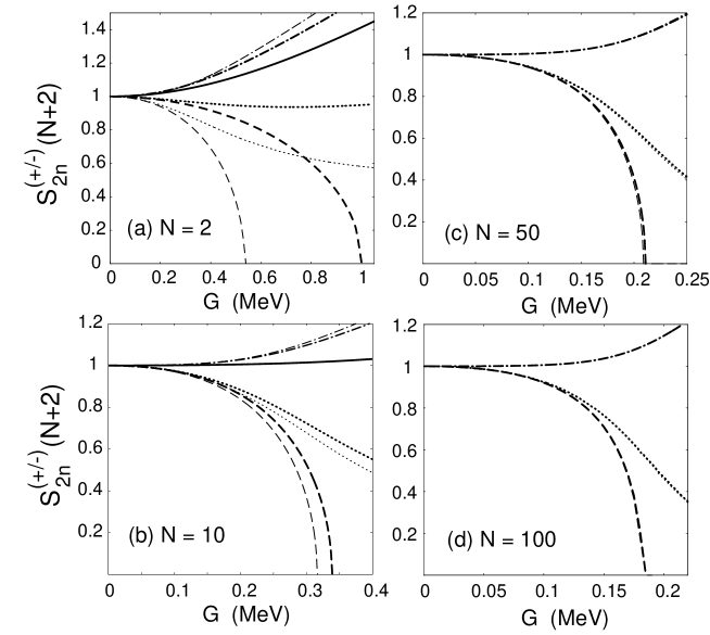
Shown in Fig. 1 are the two-particle separation energies $S_{2n}^{(\pm)}(N+2)$, which are obtained within the RPA, RRPA, and SCRPA according to Eq. (38) at $N=$ 2, 10, 50, and 100. For a comparison, the exact results, available for $N=$ 2 and 10, are also shown. For $N=$ 50 and 100 the size of the matrix makes the exact diagonalization infeasible so that the exact solutions are not available. In Ref. Duk (6) it has been analyzed in detail that the RRPA and SCRPA extend the solutions far beyond the point where the RPA collapses, and that the SCRPA predictions are the closest ones to the exact solutions. Therefore the details of these features are not repeated here. This figure shows that, for $N\leq$ 10, the consistency condition (39) is clearly violated in all the approximations under consideration. The violation is particular strong within the RPA at small $N$. It is seen that $S_{2n}^{(+)}(N+2)>S_{2n}^{(-)}(N+2)$ within the RPA and RRPA, but $S_{2n}^{(+)}(N+2)<S_{2n}^{(-)}(N+2)$ within the SCRPA. At a given value of $G$, the SCRPA predicts the smallest difference between $S_{2n}^{(+)}(N+2)$ and $S_{2n}^{(-)}(N+2)$, while the RPA gives the largest one. One can see how $S_{2n}^{(+)}(N+2)$ gets closer to $S_{2n}^{(-)}(N+2)$ as $N$ increases so that Eq. (39) is perfectly restored at $N=$ 100. The small difference between $S_{2n}^{(+)}(N+2)$ and $S_{2n}^{(-)}(N+2)$ and the better agreement with the exact result, obtained within the SCRPA even at small $N$, show that the SCRPA is the most consistent approximation among three approximations under consideration. At the same time, the quite large difference between $S_{2n}^{(+)}(N+2)$ and $S_{2n}^{(-)}(N+2)$ obtained within the RPA at small $N$ shows that the RPA is, in principle, an inconsistent theory when applied to light systems. This observation means that, GSC are important and cannot be neglected in calculations for light systems.

Refer to caption
Figure 3: Squares of matrix elements corresponding to the pair-transition probabilities as functions of pairing parameter $G$ at several values of $N$. The notations for dashed, dotted, and dash-dotted lines are as in Fig. 1. The thick and thin lines denote $B_{\mu=1}(N\rightarrow N+2)$ and $B_{\lambda=1}(N\leftarrow N+2)$, respectively.

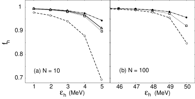
In order to see the origin of the effect due to GSC, the occupation numbers $f_{h}$ of five hole levels, which are located nearest to the Fermi level, are plotted in Fig. 2 for $N=$ 10 and 100. They are obtained by using the values of $G$ equal to 0.33 MeV and 0.17 MeV for $N=$ 10 and 100, respectively. These values are just below the collapsing points of the RPA, which are $G_{\rm crit}=$ 0.34 MeV and 0.18 MeV for $N=$ 10 and 100, respectively. The results in Fig. 2 (a) shows that the QBA, on which the RPA is based, is no longer a good approximation when $N$ is small. Indeed, the QBA means that $f_{h}=$ 1, while the value of $f_{h}$, obtained for the level just below the Fermi level, is around 0.7 within the RPA. At large $N$, e.g. $N=$ 100, the QBA is much better fulfilled as the occupation number $f_{h=1}$ is around 0.85, while those for all the other 49 hole levels are larger than 0.95 [Fig. 2 (b)]. This figure also shows that the effect of GCS, once included within the RRPA and SCRPA, makes the RRPA and SCRPA phonon operators much closer to the ideal bosons since the values of $f_{h}$ predicted by the RRPA and SCRPA for the hole level just below the Fermi level are around 0.9 and 0.95, respectively, for $N=$ 10, and larger than these values at larger $N$. The comparison of the occupation numbers predicted by the RPA, RRPA, and SCRPA again shows that the QBA is best satisfied within the SCRPA. It is interesting to notice that, while the SCRPA predicts a two-particle separation energy much closer to the exact value for $N=$ 10 as compared to the RPA [Fig. 1 (b)], the agreement between the SCRPA prediction and exact values for the occupation number $f_{h=1}$ is not as good as that offered by the RRPA.

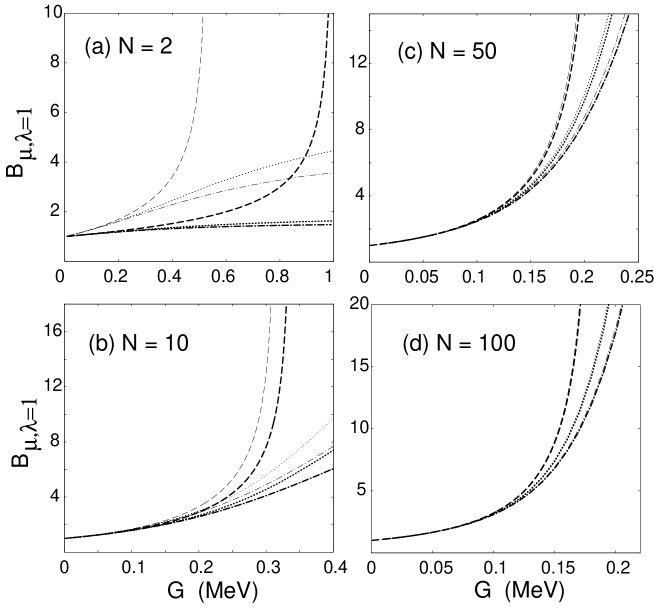
The pair-transition probabilities, shown in Fig. 3, increase with increasing $G$ as one might expect. In a similar way as that for the two-particle separation energies, the condition (43) is strongly violated within the RPA for small $N$. Combining the results on Figs. 1 and 3, it is seen that for $N\leq$ 10, neither condition (39) nor (43) holds. Like the restoration of the consistency condition (39) for two-particle separation energies, as $N$ increases the condition (43) for pair-transition probabilities is also gradually restored to become well-fulfilled at $N=$ 100.

IV Conclusions

The present paper tested the consistency of the RPA, RRPA, and SCRPA within the Richardson model. The consistency condition under consideration here is the requirement that the two-particle separation energy $S_{2n}^{(+)}(N+2)$ obtained as the energy of the first addition mode, which adds 2 particles to the $N$-particle system, should be the same as $S_{2n}^{(-)}(N+2)$ obtained as the energy of the first removal mode, which removes 2 particles from the $N+2$-particle system. The results of calculations show that this consistency condition is well fulfilled only for sufficiently large values of the particle number $N$ ($\geq$ 50 in the present model), i.e. in medium-mass and heavy systems. For light systems ($N\leq$ 10) it is found that, among the three approximations under consideration, the RPA, which has the largest deviation from the exact results at large $G$, strongly violates the consistency condition. The SCRPA agrees best with the exact solutions and also is the most consistent approximation in the sense that the above-mentioned consistency condition is well satisfied already at $N\geq$ 10 even at $G$ above the RPA collapsing point.

The results obtained in this test indicate that GSC beyond RPA becomes quite important in light systems, especially in the region close to the RPA collapsing point. They invalidate the QBA, which is assumed for the pair operators within the RPA. Therefore, in principle, the RPA predictions of the two-neutron separation energies in light neutron-rich nuclei cannot be reliable without taking the effect of GSC beyond RPA into account. From the three approximations considered in the present paper, the most consistent one, which includes this effect for light systems, turns out to be the SCRPA. Although the present test was conducted within a schematic model with doubly-fold equidistant levels, it is unlikely that this general conclusion on the inconsistency of the RPA would change when applied to realistic light nuclei. As a matter of fact, the recent calculations of the two-neutron separation energy $S_{2n}$ in 12,14Be by using the Gogny interaction have shown that the RRPA shifts the result by around 14$\%$ for 12Be, and the consistency condition (39) is not fulfilled ($N=$ 10) for both the RPA and RRPAΒ DangVM (16). An easy way to see if the RPA needs to be renormalized is to estimate the occupation numbers (31) using the backward-going amplitudes $Y$ obtained within the RPA. If there is a strong deviation of $f_{p}$ ($f_{h}$) from 0 (1), this means that the validity of the RPA is deteriorated. In the above-mentioned calculations for Be-isotopes e.g., the occupation number of the last occupied shell amounts to around 0.8 within the RPA, and increases to around 0.95 within the RRPA, showing the necessity of using the SCRPA, or at least the RRPA, instead of the RPA.

Acknowledgements.
The numerical calculations were carried out using the FORTRAN IMSL Library by Visual Numerics on the RIKEN Super Combined Cluster (RSCC) System. Thanks are due to Nicole Vinh Mau (Orsay) for fruitful discussions, and Alexander Volya (Tallahassee) for the exact solutions of the Richardson model.

References

  • (1) K. Hara, Prog. Theor. Phys. 32, 88 (1964), K. Ikeda, T. Udagawa, and H. Yamamura, Prof. Theor. Phys. 33, 22 (1965).
  • (2) D.J. Rowe, Phys. Rev. 175, 1283 (1968).
  • (3) P. Schuck and S. Ethofer, Nucl. Phys. A 212, 269 (1973)
  • (4) F. Catara, N.D. Dang, and M. Sambataro, Nucl. Phys. A 579, 1 (1994).
  • (5) J. Toivanen and J. Suhonen, Phys. Rev. Lett. 75, 410 (1995).
  • (6) J. Dukelsky and P. Schuck, Phys. Let. B464, 164 (1999); J.G. Hirsch, A. Mariano, J. Dukelsky, and P. Schuck, Ann. Phys. 296, 187 (2002).
  • (7) N. Dinh Dang, Phys. Rev. C 71, 024302 (2005).
  • (8) J.C. Pacheco and N. Vinh Mau, Phys. Rev. C 65, 044004 (2002).
  • (9) R.W. Richardson, Phys. Lett. 3, 277 (1963), Phys. Lett. 5, 82 (1963), Phys. Lett. 14, 325 (1965).
  • (10) F. Pan, J.P. Draayer, W.E. Ormand, Phys. Lett. B 422, 1 (1998).
  • (11) A. Volya, B.A. Brown, and V. Zelevinsky, Phys. Lett. B 509 (2001) 37.
  • (12) P. Ring and P. Schuck, The nuclear many-body problem (Springer, Berlin, 2000).
  • (13) J. HΓΆgaasen-Feldman, Nucl. Phys. 28, 258 (1961).
  • (14) K. Hagino and G.F. Bertsch, Nucl. Phys. A 679, 163 (2000).
  • (15) N. Dinh Dang, Eur. Phys. J. A 16, 181 (2003).
  • (16) N. Dinh Dang and N. Vinh Mau, unpublished.