Hadronic Parity Violation: an Analytic Approach

Using a recent reformulation of the analysis of nuclear parity-violation (PV) using the framework of effective field theory (EFT), we show how predictions for parity-violating observables in low energy light hadronic systems can be understood in an analytic fashion. It is hoped that such an analytic approach may encourage additional experimental work as well as add to the understanding of such parity-violating phenomena, which is all too often obscured by its description in terms of numerical results obtained from complex two-body potential codes.

1 Introduction

I never had the pleasure of meeting Dubravko Tadi$\acute{\rm c}$ , which is a shame, since he and I worked on many parallel subjects over the years. An example of this is his recent work on hypernuclear decay[1] as well as his early papers on what is usually called nuclear parity violation[2]. It is the latter which I wish to focus on in this paper, which I dedicate to Dubravko’s memory.

The cornerstone of traditional nuclear physics is the study of nuclear forces and, over the years, phenomenological forms of the nuclear potential have become increasingly sophisticated. In the nucleon-nucleon ($NN$) system, where data abound, the present state of the art is indicated, for example, by phenomenological potentials such as AV18 that are able to fit phase shifts in the energy region from threshold to 350 MeV in terms of $\sim$ 40 parameters. Progress has also been made in the description of few-nucleon systems [3]. At the same time, in recent years a new technique —effective field theory (EFT)— has been used in order to attack this problem using the symmetries of QCD [4]. In this approach the nuclear interaction is separated into long- and short-distance components. In its original formulation [5], designed for processes with typical momenta comparable to the pion mass, $Q\sim m_{\pi}$, the long-distance component is described fully quantum mechanically in terms of pion exchange, while the short-distance piece is described in terms of a small number of phenomenologically-determined contact couplings. The resulting potential [6, 7] is approaching [8, 9] the degree of accuracy of purely-phenomenological potentials. Even higher precision can be achieved at lower momenta, where all interations can be taken as short-ranged, as has been demonstrated not only in the $NN$ system [10, 11], but also in the three-nucleon system [12, 13]. Precise —$\sim 1\%$— values have been generated also for low-energy, astrophysically-important cross sections for reactions such as $n+p\rightarrow d+\gamma$ [14] and $p+p\rightarrow d+e^{+}+\nu_{e}$[15]. However, besides providing reliable values for such quantities, the use of EFT techniques allows for the a realistic estimation of the size of possible corrections.

Over the past nearly half century there has also developed a series of measurements attempting to illuminate the parity-violating (PV) nuclear interaction. Indeed the first experimental paper of which I am aware was that of Tanner in 1957 [16], shortly after the experimental confirmation of parity violation in nuclear beta decay by Wu et al. [17]. Following seminal theoretical work by Michel in 1964 [18] and that of other authors in the late 1960’s [19, 20, 21], the results of such experiments have generally been analyzed in terms of a meson-exchange picture, and in 1980 the work of Desplanques, Donoghue, and Holstein (DDH) developed a comprehensive and general meson-exchange framework for the analysis of such interactions in terms of seven parameters representing weak parity-violating meson-nucleon couplings [22]. The DDH interaction has become the standard setting by which hadronic and nuclear PV processes are now analyzed theoretically.

It is important to observe, however, that the DDH framework is, at heart, a model based on a meson-exchange picture. Provided one is interested primarily in near-threshold phenomena, use of a model is unnecessary, and one can instead represent the PV nuclear interaction in a model-independent effective-field-theoretic fashion, as recently developed by Zhu et al.[23]. In this approach, the low energy PV NN interaction is entirely short-ranged, and the most general potential depends at leading order on 11 independent operators parameterized by a set of 11 a priori unknown low-energy constants (LEC’s). When applied to low-energy ($E_{\rm cm}\leq 50$ MeV) two-nucleon PV observables, however, such as the neutron spin asymmetry in the capture reaction ${\vec{n}}+p\to d+\gamma$, the 11 operators reduce to a set of five independent PV amplitudes which may be determined by an appropriate set of measurements, as described in [23], and an experimental program which should result in the determination of these couplings is underway. This is an important goal, since such interactions are interesting not only in their own right but also as background effects entering atomic PV measurements[24] as well as experiments that use parity violation in electromagnetic interactions in order to probe nuclear structure[25].

Completion of such a low-energy program would serve at least three additional purposes:

• First, it would provide particle theorists with a set of five benchmark numbers which are in principle explainable from first principles. This situation would be analogous to what one encounters in chiral perturbation theory for pseudoscalars, where the experimental determination of the ten LEC’s appearing in the ${\cal O}(p^{4})$ Lagrangian presents a challenge to hadron structure theory. While many of the ${\cal O}(p^{4})$ LEC’s are saturated by $t$-channel exchange of vector mesons, it is not clear a priori that the analogous PV NN constants are similarly saturated (as assumed implicitly in the DDH model).

• Moreover, analysis of the PV NN LEC’s involves the interplay of weak and strong interactions in the strangeness conserving sector. A similar situation occurs in $\Delta S=1$ hadronic weak interactions, and the interplay of strong and weak interactions in this case are both subtle and only partially understood, as evidenced, e.g., by the well-known the $\Delta I=1/2$ rule enigma. The additional information in the $\Delta S=0$ sector provided by a well-defined set of experimental numbers would undoubtedly shed light on this fundamental problem.

• Finally, the information derived from the low-energy nuclear PV program would also provide a starting point for a reanalysis of PV effects in many-body systems. Until now, one has attempted to use PV observables obtained from both few- and many-body systems in order to determine the seven PV meson-nucleon couplings entering the DDH potential, and several inconsistencies have emerged. The most blatant is the vastly different value for $h_{\pi}$ obtained from the PV $\gamma$-decays of ¹⁸F, ¹⁹F and from the combination of the ${\vec{p}}p$ asymmetry and the cesium anapole moment[24]. The origin of this clash could be due to any one of a number of factors. Using the operator constraints derived from the few-body program as input into the nuclear analysis could help clarify the situation. It may be, for example, that the remaining combinations of operators not constrained by the few-body program play a more significant role in nuclei than implicitly assumed by the DDH framework. Alternatively, truncation of the model space in shell model treatments of the cesium anapole moment may be the culprit. In any case, approaching the nuclear problem from a more systematic perspective and drawing upon the results of few-body studies would undoubtedly represent an advance for the field.

The purpose of the present paper is not, however, to make the case for the effective field theory program—this has already been undertaken in [23]. Also, it is not our purpose to review the subject of hadronic parity violation—indeed there exist a number of comprehensive recent reviews of this subject[26][27][28]. However, although the basic ideas of the physics are clearly set out in these works, because the NN interaction is generally represented in terms of a somewhat forbidding two-body interaction, any calculations which are done involve state of the art potentials and are somewhat mysterious except to those priests who preach this art. Rather, in this paper, we wish to argue that this need not be the case. Below we eschew a high precision but complex nuclear wavefunction approach in favor of a simple analytic treatment which captures the flavor of the subject without the complications associated with a more rigorous calculation. We show that, provided that one is working in the low energy region, one can use a simple effective interaction approach to the PV NN interaction wherein the the parity violating NN interaction is described in terms of just five real numbers, which characterize S-P wave mixing in the spin singlet and triplet channels, and the experimental and theoretical implications can be extracted within a basic effective interaction technique, wherein the nucleon interactions are represented by short range potentials. This is justified at low energy because the scales indicated by the scattering lengths—$a_{s}\sim-20$ fm, $a_{t}\sim 5$ fm—are both much larger than the $\sim 1$ fm range of the nucleon-nucleon strong interaction. Of course, precision analysis should still be done with the best and most powerful contemporary wavefunctions such as the Argonne V18 or Bonn potentials. Nevertheless, for a simple introduction to the field, we feel that the elementary discussion given below is didactically and motivationally useful. In the next section then we present a brief review of the standard DDH formalism, since this is the basis of most analysis, as well as the EFT picture in which we shall work. Then in the following section we show how the basic physics of the NN system can be elicited in a simple analytic fashion, focusing in particular on the deuteron. With this as a basis we proceed to the parity-violating NN interaction and develop a simple analytic description of low energy PV processes. We summarize out findings in a brief concluding section

2 Hadronic Parity Violation: Old and New

The essential idea behind the conventional DDH framework relies on the fairly successful representation of the parity-conserving $NN$ interaction in terms of a single meson-exchange approach. Of course, this technique requires the use of strong interaction couplings of the lightest vector and pseudoscalar mesons

$${\cal H}_{\rm st} = ig_{\pi NN}\bar{N}\gamma_{5}\tau\cdot\pi N+g_{\rho}\bar{N}\left(\gamma_{\mu}+i{\chi_{\rho}\over 2m_{N}}\sigma_{\mu\nu}k^{\nu}\right)\tau\cdot\rho^{\mu}N$$ (1)

$$+g_{\omega}\bar{N}\left(\gamma_{\mu}+i{\chi_{\omega}\over 2m_{N}}\sigma_{\mu\nu}k^{\nu}\right)\omega^{\mu}N,$$

whose values are reasonably well determined. The DDH approach to the parity-violating weak interaction utilizes a similar meson-exchange picture, but now with one strong and one weak vertex —cf. Fig. 1.

Figure 1: Parity-violating $NN$ potential generated by meson exchange.

We require then an effective parity-violating $NNM$ Hamiltonian in analogy to Eq. (1). The process is simplified somewhat by Barton’s theorem, which requires that, in the CP-conserving limit, which we employ, exchange of neutral pseudoscalars is forbidden [29]. From general arguments, the effective Hamiltonian for such interactions must take the form

$${\cal H}_{\rm wk} = i{h_{\pi}\over\sqrt{2}}\bar{N}(\tau\times\pi)_{3}N+\bar{N}\left(h_{\rho}^{0}\tau\cdot\rho^{\mu}+h_{\rho}^{1}\rho_{3}^{\mu}+{h_{\rho}^{2}\over 2\sqrt{6}}(3\tau_{3}\rho_{3}^{\mu}-\tau\cdot\rho^{\mu})\right)\gamma_{\mu}\gamma_{5}N$$ (2)

$$+\bar{N}\left(h_{\omega}^{0}\omega^{\mu}+h_{\omega}^{1}\tau_{3}\omega^{\mu}\right)\gamma_{\mu}\gamma_{5}N-h_{\rho}^{{}^{\prime}1}\bar{N}(\tau\times\rho^{\mu})_{3}{\sigma_{\mu\nu}k^{\nu}\over 2m_{N}}\gamma_{5}N.$$

We see that there exist, in this model, seven unknown weak couplings $h_{\pi}$, $h_{\rho}^{0}$, … However, quark model calculations suggest that $h_{\rho}^{{}^{\prime}1}$ is quite small [30], so this term is usually omitted, leaving parity-violating observables described in terms of just six constants. DDH attempted to evaluate such PV couplings using basic quark-model and symmetry techniques, but they encountered significant theoretical uncertainties. For this reason their results were presented in terms of an allowable range for each, accompanied by a “best value” representing their best guess for each coupling. These ranges and best values are listed in Table 1, together with predictions generated by subsequent groups [31, 32].

	DDH[22]	DDH[22]	DZ[31]	FCDH[32]
Coupling	Reasonable Range	“Best” Value
$f_{\pi}$	$0\rightarrow 30$	+12	+3	+7
$h_{\rho}^{0}$	$30\rightarrow-81$	$-30$	$-22$	$-10$
$h_{\rho}^{1}$	$-1\rightarrow 0$	$-0.5$	+1	$-1$
$h_{\rho}^{2}$	$-20\rightarrow-29$	$-25$	$-18$	$-18$
$h_{\omega}^{0}$	$15\rightarrow-27$	$-5$	$-10$	$-13$
$h_{\omega}^{1}$	$-5\rightarrow-2$	$-3$	$-6$	$-6$

Table 1: Weak $NNM$ couplings as calculated in Refs. [22, 31, 32]. All numbers are quoted in units of the “sum rule” value $g_{\pi}=3.8\cdot 10^{-8}$.

Before making contact with experimental results, however, it is necessary to convert the $NNM$ couplings generated above into an effective parity-violating $NN$ potential. Inserting the strong and weak couplings, defined above into the meson-exchange diagrams shown in Fig. 1 and taking the Fourier transform, one finds the DDH effective parity-violating $NN$ potential

$$V^{\rm PV}_{DDH}(\vec{r}) = i{h_{\pi}g_{\pi NN}\over\sqrt{2}}\left({\tau_{1}\times\tau_{2}\over 2}\right)_{3}(\vec{\sigma}_{1}+\vec{\sigma}_{2})\cdot\left[{{\vec{p}}_{1}-{\vec{p}}_{2}\over 2m_{N}},w_{\pi}(r)\right]$$ (3)

$$-g_{\rho}\left(h_{\rho}^{0}\tau_{1}\cdot\tau_{2}+h_{\rho}^{1}\left({\tau_{1}+\tau_{2}\over 2}\right)_{3}+h_{\rho}^{2}{(3\tau_{1}^{3}\tau_{2}^{3}-\tau_{1}\cdot\tau_{2})\over 2\sqrt{6}}\right)$$

$$\quad\left((\vec{\sigma}_{1}-\vec{\sigma}_{2})\cdot\left\{{{\vec{p}}_{1}-{\vec{p}}_{2}\over 2m_{N}},w_{\rho}(r)\right\}+i(1+\chi_{V})\vec{\sigma}_{1}\times\vec{\sigma}_{2}\cdot\left[{{\vec{p}}_{1}-{\vec{p}}_{2}\over 2m_{N}},w_{\rho}(r)\right]\right)$$

$$-g_{\omega}\left(h_{\omega}^{0}+h_{\omega}^{1}\left({\tau_{1}+\tau_{2}\over 2}\right)_{3}\right)$$

$$\quad\left((\vec{\sigma}_{1}-\vec{\sigma}_{2})\cdot\left\{{{\vec{p}}_{1}-{\vec{p}}_{2}\over 2m_{N}},w_{\omega}(r)\right\}+i(1+\chi_{S})\vec{\sigma}_{1}\times\vec{\sigma}_{2}\cdot\left[{{\vec{p}}_{1}-{\vec{p}}_{2}\over 2m_{N}},w_{\omega}(r)\right]\right)$$

$$-\left(g_{\omega}h_{\omega}^{1}-g_{\rho}h_{\rho}^{1}\right)\left({\tau_{1}-\tau_{2}\over 2}\right)_{3}(\vec{\sigma}_{1}+\vec{\sigma}_{2})\cdot\left\{{{\vec{p}}_{1}-{\vec{p}}_{2}\over 2m_{N}},w_{\rho}(r)\right\}$$

$$-g_{\rho}h_{\rho}^{1^{\prime}}i\left({\tau_{1}\times\tau_{2}\over 2}\right)_{3}(\vec{\sigma}_{1}+\vec{\sigma}_{2})\cdot\left[{{\vec{p}}_{1}-{\vec{p}}_{2}\over 2m_{N}},w_{\rho}(r)\right],$$

where $w_{i}(r)=\exp(-m_{i}r)/4\pi r$ is the usual Yukawa form, $r=|{\vec{x}}_{1}-{\vec{x}}_{2}|$ is the separation between the two nucleons, and ${\vec{p}}_{i}=-i{\vec{\nabla}}_{i}$.

Nearly all experimental results involving nuclear parity violation have been analyzed using $V^{\rm PV}_{DDH}$ for the past twenty-some years. At present, however, there appear to exist discrepancies between the values extracted for the various DDH couplings from experiment. In particular, the values of $h_{\pi}$ and $h_{\rho}^{0}$ extracted from $\vec{p}p$ scattering and the $\gamma$ decay of ¹⁸F do not appear to agree with the corresponding values implied by the anapole moment of ¹³³Cs measured in atomic parity violation [33].

These inconsistencies suggest that the DDH framework may not, after all, adequately characterize the PV NN interaction and provides motivation for our reformulation using EFT. In this approach, the effective PV potential is entirely short-ranged and has the co-ordinate space form

$$V_{eff}^{PV}({\vec{r}}) = {2\over\Lambda_{\chi}^{3}}\left\{\left[C_{1}+C_{2}{\tau_{1}^{z}+\tau_{2}^{z}\over 2}\right]\left({\vec{\sigma}}_{1}-{\vec{\sigma}}_{2}\right)\cdot\{-i\vec{\nabla},f_{m}(r)\}\right.$$ (4)

$$\left.+\left[{\tilde{C}}_{1}+{\tilde{C}}_{2}{\tau_{1}^{z}+\tau_{2}^{z}\over 2}\right]i\left({\vec{\sigma}}_{1}\times{\vec{\sigma}}_{2}\right)\cdot[-i\vec{\nabla},f_{m}(r)]\right.$$

$$\left.+\left[C_{2}-C_{4}\right]{\tau_{1}^{z}-\tau_{2}^{z}\over 2}\left({\vec{\sigma}}_{1}+{\vec{\sigma}}_{2}\right)\cdot\{-i\vec{\nabla},f_{m}(r)\}\right.$$

$$\left.+\left[C_{3}\tau_{1}\cdot\tau_{2}+C_{4}{\tau_{1}^{z}+\tau_{2}^{z}\over 2}+{\cal I}_{ab}C_{5}\tau_{1}^{a}\tau_{2}^{b}\right]\left({\vec{\sigma}}_{1}-{\vec{\sigma}}_{2}\right)\cdot\{-i\vec{\nabla},f_{m}(r)\}\right.$$

$$\left.+\left[{\tilde{C}}_{3}\tau_{1}\cdot\tau_{2}+{\tilde{C}}_{4}{\tau_{1}^{z}+\tau_{2}^{z}\over 2}+{\cal I}_{ab}{\tilde{C}}_{5}\tau_{1}^{a}\tau_{2}^{b}\right]i\left({\vec{\sigma}}_{1}\times{\vec{\sigma}}_{2}\right)\cdot[-i\vec{\nabla},f_{m}(r)]\right.$$

$$\left.+C_{6}i\epsilon^{ab3}\tau_{1}^{a}\tau_{2}^{b}\left({\vec{\sigma}}_{1}+{\vec{\sigma}}_{2}\right)\cdot[-i\vec{\nabla},f_{m}(r)]\right\},$$

where

$${\cal I}^{ab}=\left(\begin{array}[]{lll}1&0&0\\ 0&1&0\\ 0&0&-2\end{array}\right),$$ (5)

and $f_{m}({\vec{r}})$ is a function which

• is strongly peaked, with width $\sim 1/m$ about $r=0$, and

• approaches $\delta^{(3)}({\vec{r}})$ in the zero width—$m\rightarrow\infty$—limit.

A convenient form, for example, is the Yukawa-like function

$$f_{m}(r)={m^{2}\over 4\pi r}\exp(-mr)$$ (6)

where $m$ is a mass chosen to reproduce the appropriate short range effects. Actually, for the purpose of carrying out actual calculations, one could just as easily use the momentum-space form of $V^{\rm PV}_{\rm SR}$, thereby avoiding the use of $f_{m}({\vec{r}})$ altogether. Nevertheless, the form of Eq. 4 is useful when comparing with the DDH potential. For example, we observe that the same set of spin-space and isospin structures appear in both $V^{\rm PV}_{eff}$ and the vector-meson exchange terms in $V^{\rm PV}_{\rm DDH}$, though the relationship between the various coefficients in $V^{\rm PV}_{eff}$ is more general. In particular, the DDH model is tantamount to assuming

$${{\tilde{C}}_{1}\over C_{1}}={{\tilde{C}}_{2}\over C_{2}}=1+\chi_{\omega},$$ (7)

$${{\tilde{C}}_{3}\over C_{3}}={{\tilde{C}}_{4}\over C_{4}}={{\tilde{C}}_{5}\over C_{5}}=1+\chi_{\rho},$$ (8)

and taking $m\sim m_{\rho},m_{\omega}$, assumptions which may not be physically realistic. Nevertheless, if this ansatz is made, the EFT and DDH results coincide provided the identifications

$$C_{1}^{DDH} = -{\Lambda_{\chi}^{3}\over 2m_{N}m_{\omega}^{2}}g_{\omega NN}h_{\omega}^{0},$$

$$C_{2}^{DDH} = -{\Lambda_{\chi}^{3}\over 2m_{N}m_{\omega}^{2}}g_{\omega NN}h_{\omega}^{1},$$

$$C_{3}^{DDH} = -{\Lambda_{\chi}^{3}\over 2m_{N}m_{\rho}^{2}}g_{\rho NN}h_{\rho}^{0},$$

$$C_{4}^{DDH} = -{\Lambda_{\chi}^{3}\over 2m_{N}m_{\rho}^{2}}g_{\rho NN}h_{\rho}^{1},$$

$$C_{5}^{DDH} = {\Lambda_{\chi}^{3}\over 4\sqrt{6}m_{N}m_{\rho}^{2}}g_{\rho NN}h_{\rho}^{2},$$

$$C_{6}^{DDH} = -{\Lambda_{\chi}^{3}\over 2m_{N}m_{\rho}^{2}}g_{\rho NN}h_{\rho}^{\prime 1}.$$

are made[23].

Before beginning our analysis of PV NN scattering, however, it is important to review the analogous PC NN scattering case, since it is more familiar and it is a useful arena wherein to compare conventional and effective field theoretic methods.

3 Parity Conserving NN Scattering

We begin our discussion with a brief review of conventional scattering theory[34]. In the usual partial wave expansion, we can write the scattering amplitude as

$$f(\theta)=\sum_{\ell}(2\ell+1)a_{\ell}(k)P_{\ell}(\cos\theta)$$ (9)

where $a_{\ell}(k)$ has the form

$$a_{\ell}(k)={1\over k}e^{i\delta(k)}\sin\delta(k)={1\over k\cot\delta(k)-ik}$$ (10)

3.1 Conventional Analysis

Working in the usual potential model approach, a general expression for the scattering phase shift $\delta_{\ell}(k)$ is[34]

$$\sin\delta_{\ell}(k)=-k\int_{0}^{\infty}dr^{\prime}r^{\prime}j_{\ell}(kr^{\prime})2m_{r}V(r^{\prime})u_{\ell,k}(r^{\prime})$$ (11)

where $m_{r}$ is the reduced mass and

$$u_{\ell,k}(r) = r\cos\delta_{\ell}(k)j_{\ell}(kr)+kr\int_{0}^{r}dr^{\prime}r^{\prime}j_{\ell}(kr^{\prime})n_{\ell}(kr)u_{\ell,k}(r^{\prime})2m_{r}V(r^{\prime})$$ (12)

$$+ kr\int_{r}^{\infty}dr^{\prime}r^{\prime}j_{\ell}(kr)n_{\ell}(kr^{\prime})u_{\ell,k}(r^{\prime})2m_{r}V(r^{\prime})$$

is the scattering wavefunction. At low energies one can characterize the analytic function $k^{2\ell+1}\cot\delta(k)$ via an effective range expansion[35]

$$k^{2\ell+1}\cot\delta_{\ell}(k)=-{1\over a}+{1\over 2}r_{e}k^{2}+\ldots$$ (13)

Then from Eq. 11 we can identify the scattering length as

$$a_{\ell}={1\over[(2\ell+1)!!]^{2}}\int_{0}^{\infty}dr^{\prime}(r^{\prime})^{2\ell+2}2m_{r}V(r^{\prime})+{\cal O}(V^{2})$$ (14)

For simplicity, we consider only S-wave interactions. Then for neutron-proton interactions, for example, one finds

$$a_{0}^{s} = -23.715\pm 0.015\,\,{\rm fm},\,\,r_{0}^{s}=2.73\pm 0.03\,\,{\rm fm}$$

$$a_{0}^{t} = 5.423\pm 0.005\,\,{\rm fm},\,\,r_{0}^{t}=1.73\pm 0.02\,\,{\rm fm}$$ (15)

for scattering in the spin-singlet and spin-triplet channels respectively. The existence of a bound state $E_{B}=-\gamma^{2}/2m_{r}$ is indicated by the presence of a pole along the positive imaginary $k$-axis—i.e. $\gamma>0$ under the analytic continuation $k\rightarrow i\gamma$—

$${1\over a_{0}}+{1\over 2}r_{0}\gamma^{2}-\gamma=0$$ (16)

We see from Eq. 15 that there is no bound state in the np spin-singlet channel, but in the spin-triplet system there exists a solution

$$\kappa={1-\sqrt{1-{2r_{0}^{t}\over a_{0}^{t}}}\over r_{0}^{t}}=45.7\,\,{\rm MeV},\quad i.e.\quad E_{B}=-2.23\,\,{\rm MeV}$$ (17)

corresponding to the deuteron.

As a specific example, suppose we utilize a simple square well potential to describe the interaction

$$V(r)=\left\{\begin{array}[]{cc}-V_{0}&r\leq R\\ 0&r>R\end{array}\right.$$ (18)

For S-wave scattering the wavefunction in the interior and exterior regions can then be written as

$$\psi^{(+)}(r)=\left\{\begin{array}[]{lc}Nj_{0}(Kr)&r\leq R\\ N^{\prime}(j_{0}(kr)\cos\delta_{0}-n_{0}(kr)\sin\delta_{0})&r>R\end{array}\right.$$ (19)

where $j_{0},n_{0}$ are spherical harmonics and the interior, exterior wavenumbers are given by $k=\sqrt{2m_{r}E}$, $K=\sqrt{2m_{r}(E+V_{0})}$ respectively. The connection between the two forms can be made by matching logarithmic derivatives at the boundary, which yields

$$k\cot\delta\simeq-{1\over R}\left[1+{1\over KRF(KR)}\right]\quad{\rm with}\quad F(x)=\cot x-{1\over x}$$ (20)

Making the effective range expansion—Eq 13—we find an expression for the scattering length

$$a_{0}=R\left[1-{\tan(K_{0}R)\over K_{0}R}\right]\quad{\rm where}\quad K_{0}=\sqrt{2m_{r}V_{0}}$$ (21)

Note that for weak potentials—$K_{0}R<<1$—this form agrees with the general result Eq. 14—

$$a_{0}=\int_{0}^{\infty}dr^{\prime}{r^{\prime}}^{2}2m_{r}V(r^{\prime})=-{2m_{r}\over 3}R^{3}V_{0}+{\cal O}(V_{0}^{2})$$ (22)

3.2 Coulomb Effects

When Coulomb interactions are included the analysis becomes somewhat more challenging. Suppose first that only same charge (e.g., proton-proton) scattering is considered and that, for simplicity, we describe the interaction in terms of a potential of the form

$$V(r)=\left\{\begin{array}[]{cc}U(r)&r<R\\ \alpha\over r&r>R\end{array}\right.$$ (23)

i.e. a strong attraction—$U(r)$—at short distances, in order to mimic the strong interaction, and the repulsive Coulomb potential—$\alpha/r$—at large distance, where $\alpha\simeq 1/137$ is the fine structure constant. The analysis of the scattering then proceeds as above but with the replacement of the exterior spherical Bessel functions by corresponding Coulomb wavefunctions $F_{0}^{+},G_{0}^{+}$

$$j_{0}(kr)\rightarrow F_{0}^{+}(r),\qquad n_{0}(kr)\rightarrow G_{0}^{+}(r)$$ (24)

whose explicit form can be found in reference [36]. For our purposes we require only the form of these functions in the limit $kr<<1$—

$$F_{0}^{+}(r) \stackrel{{\scriptstyle kr<<1}}{{\longrightarrow}} C(\eta_{+}(k))(1+{r\over 2a_{B}}+\ldots)$$

$$G_{0}^{+}(r) \stackrel{{\scriptstyle kr<<1}}{{\longrightarrow}} -{1\over C(\eta_{+}(k))}\left\{{1\over kr}\right.$$

$$+ \left.2\eta_{+}(k)\left[h(\eta_{+}(k))+2\gamma_{E}-1+\ln{r\over a_{B}}\right]+\ldots\right\}$$

(25)

Here $\gamma_{E}=0.577215..$ is the Euler constant,

$$C^{2}(x)={2\pi x\over\exp(2\pi x)-1}$$ (26)

is the usual Coulombic enhancement factor, $a_{B}=1/m_{r}\alpha$ is the Bohr radius, $\eta_{+}(k)=1/2ka_{B}$, and

$$h(\eta_{+}(k))={\rm Re}H(i\eta_{+}(k))=\eta_{+}^{2}(k)\sum_{n=1}^{\infty}{1\over n(n^{2}+\eta_{+}^{2}(k))}-\ln\eta_{+}(k)-\gamma_{E}$$ (27)

where $H(x)$ is the analytic function

$$H(x)=\psi(x)+{1\over 2x}-\ln(x)$$ (28)

Equating interior and exterior logarithmic derivatives we find

$$KF(KR) = {\cos\delta_{0}{F_{0}^{+}}^{\prime}(R)-\sin\delta_{0}{G_{0}^{+}}^{\prime}(R)\over\cos\delta_{0}F_{0}^{+}(R)-\sin\delta_{0}G_{0}^{+}(R)}$$

$$= {k\cot\delta_{0}C^{2}(\eta_{+}(k)){1\over 2a_{B}}-{1\over R^{2}}\over k\cot\delta_{0}C^{2}(\eta_{+}(k))+{1\over R}+{1\over a_{B}}\left[h(\eta_{+}(k))-\ln{a_{B}\over R}+2\gamma_{E}-1\right]}$$

(29)

Since $R<<a_{B}$ Eq. 29 can be written in the form

$$k\cot\delta_{0}C^{2}(\eta_{+}(k))+{1\over a_{B}}\left[h(\eta_{+}(k))-\ln{a_{B}\over R}+2\gamma_{E}-1\right]\simeq-{1\over a_{0}}$$ (30)

The scattering length $a_{C}$ in the presence of the Coulomb interaction is conventionally defined as[37]

$$k\cot\delta_{0}C^{2}(\eta_{+}(k))+{1\over a_{B}}h(\eta_{+}(k))=-{1\over a_{C}}+\ldots$$ (31)

so that we have the relation

$$-{1\over a_{0}}=-{1\over a_{C}}-{1\over a_{B}}(\ln{a_{B}\over R}+1-2\gamma_{E})$$ (32)

between the experimental scattering length—$a_{C}$—and that which would exist in the absence of the Coulomb interaction—$a_{0}$.

As an aside we note that, strictly speaking, $a_{0}$ is not itself an observable since the Coulomb interaction cannot be turned off. However, in the case of the pp interaction isospin invariance requires $a_{0}^{pp}=a_{0}^{nn}$ so that one has the prediction

$$-{1\over a_{0}^{nn}}=-{1\over a_{C}^{pp}}-\alpha M_{N}(\ln{1\over\alpha M_{N}R}+1-2\gamma_{E})$$ (33)

While this is a model dependent result, Jackson and Blatt have shown, by treating the interior Coulomb interaction perturbatively, that a version of this result with $1-2\gamma_{E}\rightarrow 0.824-2\gamma_{E}$ is approximately valid for a wide range of strong interaction potentials[36] and the correction indicated in Eq. 33 is essential in restoring agreement between the widely discrepant—$a_{0}^{nn}=-18.8$ fm vs. $a_{C}^{pp}=-7.82$ fm—values obtained experimentally.

Returning to the problem at hand, the experimental scattering amplitude can then be written as

$$f_{C}^{+}(k) = {e^{2i\sigma_{0}}C^{2}(\eta_{+}(k))\over-{1\over a_{C}}-{1\over a_{B}}h(\eta_{+}(k))-ikC^{2}(\eta_{+}(k))}$$ (34)

$$= {e^{2i\sigma_{0}}C^{2}(\eta_{+}(k))\over-{1\over a_{C}}-{1\over a_{B}}H(i\eta_{+}(k))}$$

where $\sigma_{0}={\rm arg}\Gamma(1-i\eta_{+}(k))$ is the Coulomb phase.

3.3 Effective Field Theory Analysis

Identical results may be obtained using effective field theory (EFT) methods and in many ways the derivation is clearer and more intuitive[38]. The basic idea here is that since we are only interested in interactions at very low energy, a scattering length description is quite adequate. From Eq. 22 we see that, at least for weak potentials, the scattering length has a natural representation in terms of the momentum space potential $\tilde{V}(\vec{p}=0)$—

$$a_{0}={m_{r}\over 2\pi}\int d^{3}rV(r)={m_{r}\over 2\pi}\tilde{V}(\vec{p}=0)$$ (35)

and it is thus natural to perform our analysis using a simple contact interation. First consider the situation that we have two particles A,B interacting only via a local strong interaction, so that the effective Lagrangian can be written as

$${\cal L}=\sum_{i=A}^{B}\Psi_{i}^{\dagger}(i{\partial\over\partial t}+{\vec{\nabla}^{2}\over 2m_{i}})\Psi_{i}-C_{0}\Psi_{A}^{\dagger}\Psi_{A}\Psi_{B}^{\dagger}\Psi_{B}+\ldots$$ (36)

The T-matrix is then given in terms of the multiple scattering series shown in Figure 1

$$T_{fi}(k)=-{2\pi\over m_{r}}f(k)=C_{0}+C_{0}^{2}G_{0}(k)+C_{0}^{3}G_{0}^{2}(k)+\ldots={C_{0}\over 1-C_{0}G_{0}(k)}$$ (37)

where $G_{0}(k)$ is the amplitude for particles $A,B$ to travel from zero separation to zero separation—i.e the propagator $D_{F}(k;\vec{r}^{\prime}=0,\vec{r}=0)$—

$$G_{0}(k)=\lim_{\vec{r}^{\prime},\vec{r}\rightarrow 0}\int{d^{3}s\over(2\pi)^{3}}{e^{i\vec{s}\cdot\vec{r}^{\prime}}e^{-i\vec{s}\cdot\vec{r}}\over{k^{2}\over 2m_{r}}-{s^{2}\over 2m_{r}}+i\epsilon}=\int{d^{3}s\over(2\pi)^{3}}{2m_{r}\over k^{2}-s^{2}+i\epsilon}$$ (38)

Equivalently $T_{fi}(k)$ satisfies a Lippman-Schwinger equation

$$T_{fi}(k)=C_{0}+C_{0}G_{0}(k)T_{fi}(k).$$ (39)

whose solution is given in Eq. 37.

Figure 2: The multiple scattering series.

The complication here is that the function $G_{0}(k)$ is divergent and must be defined via some sort of regularization. There are a number of ways by which to do this, but perhaps the simplest is to use a cutoff regularization with $k_{max}=\mu$, which simply eliminates the high momentum components of the wavefunction completely. Then

$$G_{0}(k)=-{m_{r}\over 2\pi}({2\mu\over\pi}+ik)$$ (40)

(Other regularization schemes are similar. For example, one could subtract at an unphysical momentum point, as proposed by Gegelia[39]

$$G_{0}(k)=\int{d^{3}s\over(2\pi)^{3}}({2m_{r}\over k^{2}-s^{2}+i\epsilon}+{2m_{r}\over\mu^{2}+s^{2}})=-{m_{r}\over 2\pi}(\mu+ik)$$ (41)

which has been shown by Mehen and Stewart[40] to be equivalent to the power divergence subtraction (PDS) scheme proposed by Kaplan, Savage and Wise.[38]) In any case, the would-be linear divergence is, of course, cancelled by introduction of a counterterm accounting for the omitted high energy component of the theory, which renormalizes $C_{0}$ to $C_{0}(\mu)$. That $C_{0}(\mu)$ should be a function of the cutoff is clear because by varying the cutoff energy we are varying the amount of higher energy physics which we are including in our effective description. The scattering amplitude then becomes

$$f(k)=-{m_{r}\over 2\pi}\left({1\over{1\over C_{0}(\mu)}-G_{0}(k)}\right)={1\over-{2\pi\over m_{r}C_{0}(\mu)}-{2\mu\over\pi}-ik}$$ (42)

Comparing with Eq. 10 we identify the scattering length as

$$-{1\over a_{0}}=-{2\pi\over m_{r}C_{0}(\mu)}-{2\mu\over\pi}$$ (43)

Of course, since $a_{0}$ is a physical observable, it is cutoff independent, so that the $\mu$ dependence of $1/C_{0}(\mu)$ is cancelled by the cutoff dependence in the Green’s function.

3.4 Coulomb Effects in EFT

More interesting is the case where we restore the Coulomb interaction between the particles. The derivatives in Eq. 36 then become covariant and the bubble sum is evaluated with static photon exchanges between each of the lines—each bubble is replaced by one involving a sum of zero, one, two, etc. Coulomb interactions, as shown in Figure 2.

Figure 3: The Coulomb corrected bubble.

The net result in the case of same charge scattering is the replacement of the free propagator by its Coulomb analog

$$G_{0}(k)\rightarrow G_{C}^{+}(k) = \lim_{\vec{r}^{\prime},\vec{r}\rightarrow 0}\int{d^{3}s\over(2\pi)^{3}}{\psi^{+}_{\vec{s}}(\vec{r}^{\prime}){\psi^{+}_{\vec{s}}}^{*}(\vec{r})\over{k^{2}\over 2m_{r}}-{s^{2}\over 2m_{r}}+i\epsilon}$$ (44)

$$= \int{d^{3}s\over(2\pi)^{3}}{2m_{r}C^{2}(\eta_{+}(s))\over k^{2}-s^{2}+i\epsilon}$$

where

$$\psi^{+}_{\vec{s}}(\vec{r})=C(\eta_{+}(s))e^{i\sigma_{0}}e^{i\vec{s}\cdot\vec{r}}{}_{1}F_{1}({-i\eta_{+}(s),1,isr-i\vec{s}\cdot\vec{r}})$$ (45)

is the outgoing Coulomb wavefunction for repulsive Coulomb scattering.[41] Also in the initial and final states the influence of static photon exchanges must be included to all orders, which produces the factor $C^{2}(2\pi\eta_{+}(k))\exp(2i\sigma_{0})$. Thus the repulsive Coulomb scattering amplitude becomes

$$f_{C}^{+}(k)=-{m_{r}\over 2\pi}{C_{0}C^{2}(\eta_{+}(k))\exp 2i\sigma_{0}\over 1-C_{0}{}G_{C}^{+}(k)}$$ (46)

The momentum integration in Eq. 44 can be performed as before using cutoff regularization, yielding

$$G_{C}^{+}(k)=-{m_{r}\over 2\pi}\left\{{2\mu\over\pi}+{1\over a_{B}}\left[H(i\eta_{+}(k))-\ln{\mu a_{B}\over\pi}-\zeta\right]\right\}$$ (47)

where $\zeta=\ln 2\pi-\gamma$. We have then

$$f_{C}^{+}(k)={C^{2}(\eta_{+}(k))e^{2i\sigma_{0}}\over-{2\pi\over m_{r}C_{0}(\mu)}-{2\mu\over\pi}-{1\over a_{B}}\left[H(i\eta_{+}(k))-\ln{\mu a_{B}\over\pi}-\zeta\right]}$$

$$={C^{2}(\eta_{+}(k))e^{2i\sigma_{0}}\over-{1\over a_{0}}-{1\over a_{B}}\left[h(\eta_{+}(k)-\ln{\mu a_{B}\over\pi}-\zeta\right]-ikC^{2}(\eta_{+}(k))}$$ (48)

Comparing with Eq. 34 we identify the Coulomb scattering length as

$$-{1\over a_{C}}=-{1\over a_{0}}+{1\over a_{B}}(\ln{\mu a_{B}\over\pi}+\zeta)$$ (49)

which matches nicely with Eq. 32 if a reasonable cutoff $\mu\sim m_{\pi}\sim 1/R$ is employed. The scattering amplitude then has the simple form

$$f_{C}^{+}(k)={C^{2}(\eta_{+}(k))e^{2i\sigma_{0}}\over-{1\over a_{C}}-{1\over a_{B}}H(i\eta_{+}(k))}$$ (50)

in agreement with Eq. 34.

Before moving to our ultimate goal, which is the parity violating sector, it is useful to spend some additional time focusing on the deuteron state, since this will be used in our forthcoming PV analysis and provides a useful calibration of the precision of our approach.

4 The Deuteron

Fermi was fond of asking the question “Where’s the hydrogen atom for this problem?” meaning what is the simple model that elucidates the basic physics of a given system[43]? In the case of nuclear structure, the answer is clearly the deuteron, and it is essential to have a good understanding of this simplest of nuclear systems at both the qualitative and quantitative levels. The basic static properties which we shall try to understand are indicated in Table 2. Thus, for example, from the feature that the deuteron carries unit spin with positive parity, angular momentum arguments demand that it be constructed from a combination of S- and D-wave components (a P-wave piece is forbidden from parity considerations—more about that later). Thus the wavefunction can be written in the form

$$\psi_{d}(\vec{r})={1\over\sqrt{4\pi}r}\left(u_{d}(r)+{3\over\sqrt{8}}w_{d}(r){\cal O}_{pn}\right)\chi_{t}$$ (51)

where $\chi_{t}$ is the spin-triplet wavefunction and

$${\cal O}_{pn}=\vec{\sigma}_{p}\cdot\hat{r}\vec{\sigma}_{n}\cdot\hat{r}-{1\over 3}\vec{\sigma}_{p}\cdot\vec{\sigma}_{n}$$

is the tensor operator. Here $u_{d}(r),w_{d}(r)$ represent the S-wave, D-wave components of the deuteron wavefunction, respectively. We note that

$${\cal O}_{pn}|\uparrow\uparrow> = (\cos^{2}\theta-{1\over 3})|\uparrow\uparrow>+\sin^{2}\theta e^{i2\phi}|\downarrow\downarrow>$$ (52)

$$+ \cos\theta\sin\theta e^{i\phi}(|\uparrow\downarrow>+|\downarrow\uparrow>)$$

Using

$$\int{d\Omega\over 4\pi}\hat{r}_{i}\hat{r}_{j}={1\over 3}\delta_{ij}$$ (53)

we find the normalization condition

$$1 = <\psi_{d}|\psi_{d}>=\int_{0}^{\infty}dr\int d\Omega\left[u_{d}^{2}(r)\right.$$ (54)

$$+ \left.{9\over 8}w_{d}^{2}(r)\left((\cos^{2}\theta-{1\over 3})^{2}+2\cos^{2}\theta\sin^{2}\theta+\sin^{4}\theta\right)\right]$$

$$= \int_{0}^{\infty}dr\left(u_{d}^{2}(r)+{9\over 8}w_{d}^{2}(r)(1-{2\over 9}+{1\over 9})\right)$$

$$= \int_{0}^{\infty}dr(u_{d}^{2}(r)+w_{d}^{2}(r))$$

In lowest order we can neglect the D-wave component $w_{d}(r)$. Then, in the region outside the range $r_{0}$ of the NN interaction we must have

$$r>r_{o}\qquad\left(-{1\over M}{d^{2}\over dr^{2}}+{\gamma^{2}\over M}\right)u_{d}(r)=0$$ (55)

where $\gamma=45.3$ MeV is the deuteron binding momentum defined above. The solution to Eq. 55 is given by

$$r>r_{0}\qquad u_{d}(r)\sim e^{-\gamma r}$$ (56)

However, since $1/\gamma\sim 4.3$ fm $>>r_{0}\sim$ 1 fm, it is a reasonable lowest order assumption to assume the that the deuteron wavefunction has the form Eq. 56 everywhere, so that we may take

$$\psi_{d}(r)\sim\sqrt{\gamma\over 2\pi}{1\over r}e^{-\gamma r}$$ (57)

Binding Energy	$E_{B}$	2.223 MeV
Spin-parity	$J^{P}$	$1^{+}$
Isospin	$T$	0
Magnetic Dipole Moment	$\mu_{d}$	0.856$\mu_{N}$
Electric Quadrupole Moment	$Q_{d}$	0.286 efm2
Charge Radius	$\sqrt{r_{d}^{2}}$	$\sim$ 2 fm

Table 2: Static properties of the deuteron.

Of course, we also must consider scattering states. In this case the asymptotic wavefunctions of the ${}^{3}S_{1}$ and ${}^{1}S_{0}$ states must be of the form

$$\psi^{(+)}(r)\stackrel{{\scriptstyle r\rightarrow\infty}}{{\longrightarrow}}{e^{i\delta(k)}\over kr}\sin(kr+\delta(k))={\sin kr\over kr}+{e^{ikr}\over r}t(k)$$ (58)

with

$$t(k)={1\over k}e^{i\delta(k)}\sin\delta(k)$$

being the partial wave transition amplitude. At very low energy we may use the simple effective range approximation defined above

$$k\,{\rm ctn}\delta(k)\simeq-{1\over a}$$ (59)

to write

$$t(k)\simeq{1\over-{1\over a}-ik}$$ (60)

Then we have the representation

$$\psi^{(+)}(r)\stackrel{{\scriptstyle r\rightarrow\infty}}{{\longrightarrow}}{e^{i\delta(k)}\over kr}\sin(kr+\delta(k))={\sin kr\over kr}+{e^{ikr}\over r}\left({1\over-{1\over a}-ik}\right)$$ (61)

and, comparing with a Green’s function solution to the Schrödinger equation

$$\psi^{(+)}(\vec{r})=e^{i\vec{k}\cdot\vec{r}}-{M\over 4\pi}\int d^{3}r^{\prime}{e^{ik|\vec{r}-\vec{r}^{\prime}|}\over|\vec{r}-\vec{r}^{\prime}|}U(\vec{r}^{\prime})\psi(\vec{r}^{\prime})$$ (62)

we see that the potential at low energy can be represented via the simple local potential

$$U(\vec{r})\simeq{4\pi\over M}a\delta^{3}(\vec{r})$$ (63)

which is sometimes called the zero-range approximation (ZRA) and is equivalent to the contact potential used in the EFT approach.

The relation between the scattering and bound state descriptions can be obtained by using the feature that the deuteron wavefunction must be orthogonal to its ${}^{3}S_{1}$ counterpart. This condition reads

$$0 = \int d^{3}r\psi_{d}^{\dagger}(r)\psi_{t}(r)=\sqrt{8\pi\gamma}\int_{0}^{\infty}dre^{-\gamma r}\left({1\over k}\sin kr+e^{ikr}t_{t}(k)\right)$$ (64)

$$= \sqrt{8\pi\gamma}\left({1\over\gamma^{2}+k^{2}}+{1\over\gamma-ik}t_{t}(k)\right)={\sqrt{8\pi\gamma}\over\gamma-ik}\left({1\over\gamma+ik}+{1\over-{1\over a_{t}}-ik}\right)$$

which requires that $\gamma=1/a_{t}$. This necessity is also clear from the already mentioned feature that the deuteron represents a pole in $t_{t}(k)$ in the limit as $k\rightarrow i\gamma$—i.e., $-1/a_{t}+\gamma=0$. Since ${1\over\gamma}\sim 4.3$ fm, this equality holds to within 20% or so and indicates the precision of our approximation. In spite of this roughness, there is much which can be learned from this simple analytic approach.

We begin with the charge radius, which is defined via

$$<r_{d}^{2}>=<r_{p}^{2}>+\int d^{3}r{1\over 4}r^{2}|\psi_{d}(r)|^{2}$$ (65)

Note here that we have included the finite size of the proton, since it is comparable to the deuteron size and have scaled the wavefunction contribution by a factor of four since $\vec{r}_{p}={1\over 2}\vec{r}$. Performing the integration, we have

$$\int d^{3}r{1\over 4}r^{2}|\psi_{d}(r)|^{2}=\pi\int_{0}^{\infty}drr^{2}u^{2}(r)={1\over 8\gamma^{2}}$$ (66)

and, since $<r_{p}^{2}>\simeq 0.65$ fm² we find

$$\sqrt{<r_{d}^{2}>}=\sqrt{0.65+{1\over 8\gamma^{2}}}\,\,{\rm fm}\simeq 1.8\,\,{\rm fm}$$ (67)

which is about 10% too low and again indicates the roughness of our approximation.

Now consider the magnetic moment, for which the relevant operator is

$$\vec{M} = {e\over 2M}\left(\mu_{p}\vec{\sigma}_{p}+\mu_{n}\vec{\sigma}_{n}\right)+{e\over 2M}\vec{L}_{p}$$ (68)

$$= {e\over 4M}\left(\vec{J}+\mu_{V}(\vec{\sigma}_{p}-\vec{\sigma}_{n})+(\mu_{S}-{1\over 2})(\vec{\sigma}_{p}+\vec{\sigma}_{n})\right)$$

where $\vec{J}=\vec{L}+{1\over 2}(\vec{\sigma}_{p}+\vec{\sigma}_{n})$ is the total angular momentum, $\mu_{V}=\mu_{p}-\mu_{n}=4.70$, $\mu_{S}=\mu_{p}+\mu_{n}=0.88$ are the isovector, isoscalar moments, and the “extra” factor of $1/2$ associated with the orbital angular momentum comes from the obvious identity $\vec{L}_{p}=\vec{L}/2$. We find then

$${e\over 2M}\mu_{d} = <\psi_{d};1,1|M_{3}|\psi_{d};1,1>={e\over 4M}\left[1+(2\mu_{S}-1)<\psi_{d};1,1|S_{3}|\psi_{d};1,1>\right]$$ (69)

$$= {e\over 4M}\left[1+(2\mu_{S}-1)\int d^{3}r(u_{d}^{2}(r)+{9\over 8}w^{2}(r)\left((\cos^{2}\theta-{1\over 3})^{2}-\sin^{4}\theta\right)\right]$$

$$= {e\over 2M}\left[\mu_{S}-{3\over 2}(\mu_{S}-{1\over 2})\int_{0}^{\infty}drw_{d}^{2}(r)\right]$$

In the lowest order approximation—neglecting the D-wave component of the deuteron—we find

$$<1,1|M_{3}|1,1>\simeq\mu_{S}{e\over 2M}$$ (70)

and this prediction—$\mu_{d}=\mu_{S}=0.88\mu_{N}$—is in good agreement with the experimental value $\mu_{d}^{exp}=0.856\mu_{N}$.

4.1 D-Wave Effects

A second static observable is the quadrupole moment $Q_{d}$, which is a measure of deuteron oblateness. In this case a pure S-wave picture predicts a spherical shape so that $Q_{d}=0$. Thus, in order to generate a quadrupole moment, we must introduce a D-wave piece of the wavefunction. Now, just as we related the $\ell=0$ wavefunction to the np scattering in the spin triplet state, we can relate the D-wave component to the scattering amplitude provided we include spin. Thus, if we write the general scattering matrix consistent with time reversal and parity-conservation as[43]

$${\cal M}(\vec{k}^{\prime},\vec{k}) = \alpha+\beta\vec{\sigma}_{p}\cdot\hat{n}\vec{\sigma}_{n}\cdot\hat{n}+\rho(\vec{\sigma}_{p}+\vec{\sigma}_{n})\cdot\hat{n}$$ (71)

$$+ (\kappa+\lambda)\vec{\sigma}_{p}\cdot\hat{n}_{+}\vec{\sigma}_{n}\cdot\hat{n}_{-}+(\kappa-\lambda)\vec{\sigma}_{p}\cdot\hat{n}_{-}\vec{\sigma}_{n}\cdot\hat{n}_{+}$$

where

$$\hat{n}_{\pm}={\vec{k}\pm\vec{k}^{\prime}\over|\vec{k}\pm\vec{k}^{\prime}|},\qquad\hat{n}={\vec{k}\times\vec{k}^{\prime}\over|\vec{k}\times\vec{k}^{\prime}|},$$

we can represent the asymptotic scattering wavefunction via

$$\psi(r)\stackrel{{\scriptstyle r\rightarrow\infty}}{{\longrightarrow}}e^{i\vec{k}\cdot\vec{r}}+{\cal M}(-i\vec{\nabla},\vec{k}){e^{ikr}\over r}$$ (72)

A useful alternative form for ${\cal M}$ can be found via the identity

$$\vec{\sigma}_{p}\cdot\hat{n}\vec{\sigma}_{n}\cdot\hat{n}=\vec{\sigma}_{p}\cdot\vec{\sigma}_{n}-\vec{\sigma}_{p}\cdot\hat{n}_{+}\vec{\sigma}_{n}\cdot\hat{n}_{+}-\vec{\sigma}_{p}\cdot\hat{n}_{-}\vec{\sigma}_{n}\cdot\hat{n}_{-}$$ (73)

and, using the deuteron spin vector $\vec{S}={1\over 2}(\vec{\sigma}_{p}+\vec{\sigma}_{n})$, it is easy to see that

$${\cal M}(\vec{k}^{\prime},\vec{k})=-a_{t}+{1\over M^{2}}\left[c^{\prime}\vec{S}\cdot\vec{k}\times\vec{k}^{\prime}+g_{1}(\vec{S}\cdot(\vec{k}+\vec{k}^{\prime}))^{2}+g_{2}(\vec{S}\cdot(\vec{k}-\vec{k}^{\prime}))^{2}\right]$$ (74)

where

$$c^{\prime}={2\rho M^{2}\over k^{2}\sin\theta},\quad g_{1}={(\kappa-\beta+\lambda)M^{2}\over 2k^{2}\cos^{2}{\theta\over 2}},\quad g_{2}={(\kappa-\beta-\lambda)M^{2}\over 2k^{2}\sin^{2}{\theta\over 2}}$$

Then, since in the ZRA

$$\vec{k}^{\prime}\rightarrow-i\vec{\nabla}\delta^{3}(\vec{r}),\qquad\vec{k}\rightarrow\delta^{3}(\vec{r})\cdot-i\vec{\nabla}$$ (75)

we find the effective local potential

$$U(\vec{r}) = {4\pi\over M}\left[a_{t}\delta^{3}(\vec{r})+{c^{\prime}\over M^{2}}\epsilon_{ijk}S_{i}\nabla_{j}\delta^{3}(\vec{r})\nabla_{k}\right.$$

$$+ \left.{1\over 2M^{2}}S_{ij}\left((g_{1}+g_{2})\{\nabla_{i}\nabla_{j},\delta^{3}(\vec{r})\}+(g_{1}-g_{2})(\nabla_{i}\delta^{3}(\vec{r})\nabla_{j}+\nabla_{j}\delta^{3}(\vec{r})\nabla_{i})\right)\right]$$

(76)

where

$$S_{ij}=S_{i}S_{j}+S_{j}S_{i}-{4\over 3}\delta_{ij}$$ (77)

Using the Green’s function representation—Eq. 72, the asymptotic form of the triplet scattering wavefunction becomes

$$\psi(r)\stackrel{{\scriptstyle r\rightarrow\infty}}{{\longrightarrow}}e^{i\vec{k}\cdot\vec{r}}-\left(a_{t}+{g_{1}+g_{2}\over 2M^{2}}S_{ij}\nabla_{i}\nabla_{j}\right){e^{ikr}\over r}\chi_{t}$$ (78)

and, by continuing to the value $k\rightarrow i\gamma$, we can represent the deuteron wavefunction as

$$\psi_{d}(r)\sim\sqrt{\gamma\over 2\pi}\left(1+{g_{1}+g_{2}\over 2M^{2}a_{t}}S_{ij}\nabla_{i}\nabla_{j}\right){1\over r}e^{-\gamma r}\chi_{t}$$ (79)

A little work shows that this can be written in the equivalent form

$$\psi_{d}(r) \sim \sqrt{\gamma\over 2\pi}\left[1+{g_{1}+g_{2}\over 2M^{2}a_{t}}{\cal O}_{pn}\left({d^{2}\over dr^{2}}-{1\over r}{d\over dr}\right)\right]{1\over r}e^{-\gamma r}\chi_{t}$$ (80)

$$= \sqrt{\gamma\over 2\pi}\left[1+{g_{1}+g_{2}\over 2M^{2}a_{t}}{\cal O}_{pn}\left({3\over r^{2}}+{3\gamma\over r}+\gamma^{2}\right)\right]{1\over r}e^{-\gamma r}\chi_{t}$$

Here the asymptotic ratio of S- and D-wave amplitudes is an observable and is denoted by

$$\eta={A_{D}\over A_{S}}={\sqrt{2}(g_{1}+g_{2})\over 3M^{2}a_{t}^{3}}$$ (81)

This quantity has been determined experimentally from elastic dp scattering and from neutron stripping reactions to be[44]

$$\eta=0.0271\pm 0.0004,\quad i.e.,\quad g_{1}+g_{2}=105\,\,{\rm fm}$$

Defining the quadrupole operator

$$Q_{ij}\equiv{e\over 4}(3r_{i}r_{j}-\delta_{ij}r^{2})$$

and using

$$\int{d\Omega\over 4\pi}\hat{r}_{i}\hat{r}_{j}\hat{r}_{k}\hat{r}_{\ell}={1\over 15}(\delta_{ij}\delta_{k\ell}+\delta_{i\ell}\delta_{jk}+\delta_{ik}\delta_{j\ell})$$ (82)

we note

$$\int d^{3}r\psi_{d}^{*}(\vec{r})Q_{ij}\psi_{d}(\vec{r})\simeq 2e\int d^{3}r\chi_{t}^{\dagger}{1\over r}u(r)Q_{ij}{(g_{1}+g_{2})\gamma\over 2M^{2}}{\cal O}_{pn}\left({3\over r^{3}}+{3\gamma\over r^{2}}+{\gamma^{2}\over r}\right)u(r)\chi_{t}$$ (83)

$$= {3e\over 2}\cdot{1\over 15}{g_{1}+g_{2})\gamma\over 2M^{2}}{\gamma\over 2\pi}\chi_{t}^{\dagger}\left(\sigma_{pi}\sigma_{nj}+\sigma_{pj}\sigma_{ni}-{2\over 3}\delta_{ij}\vec{\sigma}_{p}\cdot\vec{\sigma}_{n}\right)\chi_{t}$$

$$\times 4\pi\int_{0}^{\infty}dre^{-2\gamma r}(3+3\gamma r+\gamma^{2}r^{2})$$

$$= {1\over 5}{e(g_{1}+g_{2})\gamma^{2}\over 2M^{2}}\chi_{t}^{\dagger}\left(\sigma_{pi}\sigma_{nj}+\sigma_{pj}\sigma_{ni}-{2\over 3}\delta_{ij}\vec{\sigma}_{p}\cdot\vec{\sigma}_{n}\right)\chi_{t}\left({3\over 2\gamma}+{3\gamma\over(2\gamma)^{2}}+{2\gamma^{2}\over(2\gamma)^{3}}\right)$$

$$= {e(g_{1}+g_{2})\gamma\over 4M^{2}}\chi_{t}^{\dagger}\left(\sigma_{pi}\sigma_{nj}+\sigma_{pj}\sigma_{ni}-{2\over 3}\delta_{ij}\vec{\sigma}_{p}\cdot\vec{\sigma}_{n}\right)\chi_{t}$$

Then the quadrupole moment is found to be

$$Q_{d}^{\rm th}=<\psi_{d};1,1|Q_{zz}|\psi_{d};1,1>={e(g_{1}+g_{2})\over 3a_{t}M^{2}}\simeq 0.28\,\,e\,{\rm fm}^{2},$$ (84)

in good agreement with the experimental value

$$Q_{d}^{\rm exp}=0.286\,\,e\,{\rm fm}^{2}$$

From its definition, we observe that the quadrupole moment would vanish for a spherical (purely S-wave) deuteron and that a positive value indicates a slight elongation along the spin axis.

Note that in interpreting the meaning of the D-wave piece of the deuteron wavefunction one often sees things described in terms of the D-state probability

$$P_{D}=\int_{0}^{\infty}drw^{2}(r)$$

However, since

$$\int d^{3}r({3\over r^{2}}+{3\gamma\over r}+\gamma^{2})^{2}\exp(-2\gamma r)$$ (85)

diverges while in reality the D-wave function $w_{d}(r)$ must vanish as $r\rightarrow 0$, it is clear that the connection between the asymptotic amplitude $\eta$ and the D-state probability $P_{D}$ must be model dependent. Nevertheless, the D-state piece is a small but important component of the deuteron wavefunction. As one indication of this, let’s return to the magnetic moment calculation and insert the D-wave contribution. We find then

$$\mu_{d}=\mu_{S}-{3\over 2}(\mu_{S}-{1\over 2})P_{D}$$ (86)

If we insert the experimental value $\mu_{d}=0.857$ we find $P_{D}\simeq 0.04$ which can now be used in other venues. However, it should be kept in mind that this analysis is only approximate, since we have neglected relativisitic corrections, meson exchange currents, etc.

Of course, static properties represent only one type of probe of deuteron structure. Another is provided by the use of electromagnetic interactions, for which a well-studied case is photodisintegration—$\gamma d\rightarrow np$—or radiative capture—$np\rightarrow d\gamma$—which are related by time reversal invariance.

5 Parity Conserving Electromagnetic Interaction: $np\leftrightarrow d\gamma$

An important low energy probe of deuteron structure can be found within the electromagnetic transtion $np\leftrightarrow d\gamma$. Here the np scattering states include both spin-singlet and -triplet components and we must include a bound state—the deuteron. For simplicity, we represent the latter by purely the dominant S-wave component, which has the form

$$\psi_{d}(r)=\sqrt{\gamma\over 2\pi}{1\over r}e^{-\gamma r},\quad{\rm or}\quad\psi_{d}(q)={\sqrt{8\pi\gamma}\over\gamma^{2}+q^{2}}$$ (87)

Since we are considering an electromagnetic transition at very low energy we can be content to include only the lowest—E1, M1, and E2—mutipoles, which are described by the Hamiltonian[42]

$$H={es_{0}}\hat{\epsilon}_{\gamma}\cdot\left[\pm i{1\over 2}\vec{r}+{1\over 4M}\hat{s}_{\gamma}\times\left(\mu_{V}(\vec{\sigma}_{p}-\vec{\sigma}_{n})+(\mu_{S}-{1\over 2})(\vec{\sigma}_{p}+\vec{\sigma}_{s})\right)-{i\over 8}\vec{r}\vec{r}\cdot\vec{k}\right]$$ (88)

Here $\vec{s}_{\gamma}$ is the photon momentum, $\mu_{V},\mu_{S}=\mu_{p}\pm\mu_{n}$ are the isoscalar, isovector magnetic moments, and we have used Siegert’s theorem to convert the conventional $\vec{p}\cdot\vec{A}/M$ interaction into the E1 form given above. The $\pm$ in front of the E1 operator depends upon whether the $np\rightarrow d\gamma$ or $\gamma d\rightarrow np$ reaction is under consideration. The electromagnetic transition amplitude then can be written in the form

$${\rm Amp} = \chi_{f}^{\dagger}\left[\hat{\epsilon}_{\gamma}\times\hat{s}_{\gamma}\cdot\left(G_{M1V}(\vec{\sigma}_{p}-\vec{\sigma}_{n})+G_{M1S}(\vec{\sigma}_{p}+\vec{\sigma}_{n})\right)\right.$$ (89)

$$+ \left.G_{E1}\hat{\epsilon}_{\gamma}\cdot\hat{k}+G_{E2}\left(\vec{\sigma}_{p}\cdot\hat{\epsilon}_{\gamma}\vec{\sigma}_{n}\cdot\hat{s}_{\gamma}+\vec{\sigma}_{n}\cdot\hat{\epsilon}_{\gamma}\vec{\sigma}_{p}\cdot\hat{s}_{\gamma}\right)\right]\chi_{i}$$

The leading parity-conserving transition at near-threshold energy is then the isovector M1 amplitude—$G_{M1V}$—which connects the ${}^{3}S_{1}$ deuteron to the ${}^{1}S_{0}$ scattering state of the np system. From Eq. 88 we identify

$$G_{M1V}={es_{0}\mu_{V}\over 4M}\int d^{3}r\psi_{{}^{1}S_{0}}^{(-)*}(kr)\psi_{d}(r)$$ (90)

Using the asymptotic form

$$\psi_{{}^{1}S_{0}}^{(-)}(kr)={e^{-i\delta_{s}}\over kr}(\sin kr\cos\delta_{s}+\cos kr\sin\delta_{s})$$ (91)

the radial integral becomes

$$\int d^{3}r\psi_{{}^{1}S_{0}}^{(-)*}(kr)\psi_{d}(r) = {4\pi e^{i\delta_{s}}\over k}\int_{0}^{\infty}(\sin kr\cos\delta_{s}+\cos kr\sin\delta_{s})e^{-\gamma r}$$ (92)

$$= {4\pi e^{i\delta_{s}}\over k(k^{2}+\gamma^{2})}(k\cos\delta_{s}+\gamma\sin\delta_{s})$$

Since by energy conservation

$$s_{0}={k^{2}+\gamma^{2}\over M}$$

we can use the lowest order effective range values for the scattering phase shift to this result in the form

$$G_{M1V}={e\mu_{V}\sqrt{8\pi\gamma}e^{-i{\rm tan}^{-1}ka_{s}}(1-\gamma a_{s})\over 4M^{2}\sqrt{1+k^{2}a_{s}^{2}}}$$ (93)

Note here that the phase of the amplitude is required by the Fermi-Watson theorem, which follows from unitarity.

The M1 cross section is then found by squaring and mutiplying by phase space. In the case of radiative capture this is found to be

$$\Gamma_{np\rightarrow d\gamma}={1\over|\vec{v}_{rel}|}\int{d^{3}s\over(2\pi)^{3}2s_{0}}2\pi\delta(s_{0}-{\gamma^{2}\over M}-{k^{2}\over M})\sum_{\lambda_{\gamma}}{1\over 4}{\rm Tr}P_{t}TT^{\dagger}$$ (94)

Here

$$\sum_{\lambda_{\gamma}}{1\over 4}{\rm Tr}P_{t}TT^{\dagger} = {|G_{M1V}|^{2}\over 4}{\rm Tr}{1\over 4}(3+\vec{\sigma}_{1}\cdot\vec{\sigma}_{2})\hat{\epsilon}^{*}_{\gamma}\times\hat{s}_{\gamma}\cdot(\vec{\sigma}_{p}-\vec{\sigma}_{n})\hat{\epsilon}_{\gamma}\times\hat{s}_{\gamma}\cdot(\vec{\sigma}_{p}-\vec{\sigma}_{n})$$ (95)

$$= \sum_{\lambda_{\gamma}}|G_{M1V}|^{2}\hat{\epsilon}^{*}_{\gamma}\times\hat{s}_{\gamma}\cdot\hat{\epsilon}_{\gamma}\times\hat{s}_{\gamma}=2|G_{M1V}|^{2}$$

yielding

$$\sigma_{M1}(np\rightarrow d\gamma)={s_{0}\over 2\pi|\vec{v}_{rel}|}2|G_{M1V}|^{2}={2\pi\alpha\mu_{V}^{2}\gamma(1-\gamma a_{s})^{2}(k^{2}+\gamma^{2})\over M^{5}(1+k^{2}a_{s}^{2})}$$ (96)

Putting in numbers we find that for an incident thermal neutrons with relative velocity $|\vec{v}_{rel}|=2200$ m/sec. the predicted cross section is about 300 mb which is about 10% smaller than the experimental value

$$\sigma_{exp}=334\pm 0.1\,\,{\rm mb}$$

The discrepancy is due to our omission of two-body effects (meson exchange currents) as shown by Riska and Brown[45].

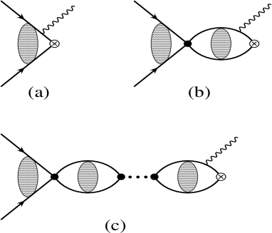
Figure 4: EFT diagrams used in order to calculate the radiative capture reaction $np\rightarrow d\gamma$.

In a corresponding EFT description of this process, we must calculate the diagrams shown in Figure 1. There is a subtlety here which should be noted. Strictly speaking, as shown by Kaplan, Savage, and Wise[46] the symbol $\otimes$ in these diagrams should be interpreted as creation or annihilation of the deuteron with wavefunction renormalization

$$\sqrt{Z}=\left({d\Sigma(E)\over dE}\right)_{E=-B}^{-{1\over 2}}$$ (97)

followed by propagation via

$${1\over{k^{2}\over M}+{\gamma^{2}\over M}}$$

However, since in lowest order we have

$$\left({d\Sigma(E)\over dE}\right)_{E=-B}^{-{1\over 2}}={\sqrt{8\pi\gamma}\over M}$$ (98)

we find for the product

$$\sqrt{Z}\cdot{1\over{k^{2}\over M}+{\gamma^{2}\over M}}={\sqrt{8\pi\gamma}\over k^{2}+\gamma^{2}}$$ (99)

which is the deuteron wavefunction in momentum space. Thus in our discussion below we shall use this substitution rather that writing the wavefunction normalization times propagator product. From Figure 4a then we find

$$G_{M1V}^{a}={es_{0}\mu_{V}\over 4M}\int{d^{3}q\over(2\pi)^{3}}\psi_{\vec{k}}^{(0)*}(\vec{q})\psi_{d}(\vec{q})$$ (100)

Since $\psi_{\vec{k}}^{(0)*}(\vec{q})=(2\pi)^{3}\delta^{3}(\vec{k}-\vec{q})$ we have

$$G_{M1V}^{a}={es_{0}\mu_{V}\over 4M}{\sqrt{8\pi\gamma}\over\gamma^{2}+k^{2}}$$ (101)

On the other hand from Figures 4b+c we find

$$G_{M1V}^{b+c}={es_{0}\mu_{V}\over 4M}\left({C_{0s}\over 1-C_{0s}G_{0}(k)}\right)^{*}\int{d^{3}q\over(2\pi)^{3}}G_{0}(\vec{r}=0,\vec{q})\psi_{d}(q)$$ (102)

Since

$$G_{0}(\vec{r}=0,\vec{q})={1\over{k^{2}\over M}-{q^{2}\over M}+i\epsilon}$$ (103)

this becomes

$$G_{M1V}^{b+c} = {es_{0}\mu_{V}\over 4M}\left({C_{0s}\over 1-C_{0s}G_{0}(k)}\right)^{*}\int{d^{3}q\over(2\pi)^{3}}{\sqrt{8\pi\gamma}\over(q^{2}+\gamma^{2})({k^{2}\over M}-{q^{2}\over M}+i\epsilon)}$$ (104)

$$= {es_{0}\mu_{V}\over 4M}\left({C_{0s}\over 1-C_{0s}G_{0}(k)}\right)^{*}{\sqrt{8\pi\gamma}\over\gamma^{2}+k^{2}}(G_{0}(k)-G_{0}(i\gamma))$$

$$= {es_{0}\mu_{V}\over 4M}\left({C_{0s}\over 1-C_{0s}G_{0}(k)}\right)^{*}{\sqrt{8\pi\gamma}\over\gamma^{2}+k^{2}}{M\over 4\pi}(-ik-\gamma)$$

Adding the two contributions we have

$$G_{M1V} = {es_{0}\mu_{V}\over 4M}{\sqrt{8\pi\gamma}\over\gamma^{2}+k^{2}}\left[1-\left({-\gamma-ik\over{-1\over a_{s}}-ik}\right)\right]$$ (105)

$$= {es_{0}\mu_{V}\over 4M}{\sqrt{8\pi\gamma}\over\gamma^{2}+k^{2}}\left({1-\gamma a_{s}\over 1+ika_{s}}\right)$$

which agrees completely with Eq. 93 obtained via conventional coordinate space procedures. Of course, we still have a $\sim 10\%$ discrepancy with the experimental cross section, which is handled by inclusion of a four-nucleon M1 counterterm connecting ${}^{3}S_{1}$ and ${}^{1}S_{0}$ states—

$${\cal L}_{2}^{EM}=eL_{1}^{M1V}(N^{T}\vec{P}\cdot\vec{B}N)^{\dagger}(N^{T}P_{3}N)$$ (106)

where here the $P_{i}$ represent relvant projection operators[47].

As the energy increases above threshold, it is necessary to include the corresponding P-conserving E1 multipole—

$${\rm Amp}=G_{E1}\hat{\epsilon}_{\gamma}\cdot\vec{k}\chi_{t}^{\dagger}\chi_{t}$$ (107)

In this case the matrix element involves the np ³P-wave final state and, neglecting final state interactions in this channel, the matrix element is given by

$$G_{E1}\vec{k}={es_{0}\over 2}\int d^{3}r\psi_{\vec{k}}^{(0)*}(r)\vec{r}\psi_{d}(r)$$ (108)

The radial integral can be found via

$$-i\vec{k}\cdot\int d^{3}re^{-i\vec{k}\cdot\vec{r}}\vec{r}\psi_{d}(r) = {d\over d\lambda}_{|_{\lambda=1}}\sqrt{\gamma\over 2\pi}\int d^{3}re^{-i\vec{k}\cdot\vec{r}\lambda}{1\over r}e^{-\gamma r}$$ (109)

$$= {d\over d\lambda}_{|_{\lambda=1}}{\sqrt{8\pi\gamma}\over\gamma^{2}+k^{2}\lambda^{2}}={-2k^{2}\sqrt{8\pi\gamma}\over(k^{2}+\gamma^{2})^{2}}$$

Equivalently using EFT methods we have

$$\int{d^{3}q\over(2\pi)^{3}}\psi^{(0)*}_{\vec{k}}(\vec{q})\vec{\nabla}_{\vec{q}}\psi_{d}(q)={-2i\sqrt{8\pi\gamma}\vec{k}\over(k^{2}+\gamma^{2})^{2}}$$ (110)

In either case

$$G_{E1}={-ies_{0}\sqrt{8\pi\gamma}\over(k^{2}+\gamma^{2})^{2}}$$ (111)

and the corresponding cross section is

$$\sigma_{E1}(np\rightarrow d\gamma) = {1\over 4}{3s_{0}\over 2\pi|\vec{v}_{rel}|}\int{d\Omega_{\hat{s}}\over 4\pi}(\vec{k}\cdot\vec{k}-(\vec{k}\cdot\hat{s})^{2}){e^{2}8\pi\gamma s_{0}^{2}\over(k^{2}+\gamma^{2})^{4}}$$ (112)

$$= {8\pi\alpha k^{2}\gamma\over|\vec{v}_{rel}|M^{3}(k^{2}+\gamma^{2})}$$

It is important to note that we can easily find the corresponding photodisintegration cross sections by multiplying by the appropriate phase space. For unpolarized photons we have

$$\sigma(\gamma d\rightarrow np) = {1\over 3\cdot 2}{1\over 2s_{0}}\int{d^{3}k\over(2\pi)^{3}}\sum_{\lambda_{\gamma}}2\pi\delta(s_{0}-{\gamma^{2}\over M}-{k^{2}\over M})|{\rm Amp}|^{2}$$ (113)

$$= {Mk\over 24\pi s_{0}}\sum_{\lambda_{\gamma}}\int{d\Omega_{\hat{k}}\over 4\pi}|{\rm Amp}|^{2}$$

Using the results obtained above for radiative capture—

$$\sum_{\lambda_{\gamma}}|{\rm Amp}|^{2}=8|G_{M1V}|^{2}+3(\vec{k}\cdot\vec{k}-(\vec{k}\cdot\hat{s})^{2})|G_{E1}|^{2}$$ (114)

we find the photodisintegration cross sections to be

$$\sigma_{M1}(\gamma d\rightarrow np)={2\pi\alpha\over 3M^{2}}{(1-a_{s}\gamma)^{2}\mu_{V}^{2}k\gamma\over(k^{2}+\gamma^{2})(1+k^{2}a_{0}^{2})},\quad\sigma_{E1}(\gamma d\rightarrow np)={8\pi\alpha\gamma k^{3}\over 3(k^{2}+\gamma^{2})^{3}}$$ (115)

Although the leading electromagnetic physics is controlled, as we have seen, by the isovector M1 and E1 amplitudes, there exist small but measurable isoscalar M1 and E2 transitions[48],[49],[50]. In the former case the transition is between the S-wave (D-wave) deuteron ground state and into the ${}^{3}S_{1}({}^{3}D)$ scattering state. The amplitude $G_{M1S}$ is small because of the smallness of $\mu_{S}-{1\over 2}$ and because of the orthogonality restriction. In the case of $G_{E2}$, the result is suppressed by the requirement for transfer of two units of angular momentum, so that the transition must be between S- and D-wave components of the wavefunction.

We first evaluate the isoscalar M1 amplitude, which from Eq. 88 is given by (cf. Eq. 69)

$$G_{M1S} = {e\over 2M}(\mu_{S}-{1\over 2})<\psi_{d};1,1|S_{3}|\psi_{d},1,1>$$ (116)

$$= {e\over 2M}(\mu_{S}-{1\over 2})\int_{0}^{\infty}dr(u_{d}(r)u_{t}(r)-{1\over 2}w_{d}(r)w_{t}(r))$$

$$= -{e\over 2M}(\mu_{S}-{1\over 2}){3\over 2}\int_{0}^{\infty}drw_{t}(r)w_{d}(r)$$

where the last form was fouind using the orthogonality condition. In order to estimate the latter, we follow Danilov in assuming that, since the radial integral is short-distance dominated, the D-wave deuteron and scattering pieces are related by a simple constant[51], which, using orthogonality, must be given by

$$w_{t}(r)\simeq-a_{t}\sqrt{2\pi\over\gamma}w_{d}(r)$$ (117)

The matrix element then becomes

$$G_{M1S}\simeq{e\over 2M}(\mu_{S}-{1\over 2}){3\over 2}P_{D}a_{t}$$ (118)

Likewise, using Eq. 82 we note that

$$\int d^{3}r\left({1\over r}u_{t}(r)+{3\over\sqrt{8}}{\cal O}_{pn}{1\over r}w_{t}(r)\right)\vec{r}\cdot\hat{\epsilon}_{\gamma}\vec{r}\cdot\hat{s}_{\gamma}\psi_{d}(\vec{r})$$

$$= {3\over\sqrt{8}}{1\over 15}\int_{0}^{\infty}drr^{2}(u_{t}(r)w_{d}(r)+w_{t}(r)u_{d}(r))\left[\vec{\sigma}_{p}\cdot\hat{\epsilon}_{\gamma}\vec{\sigma}_{n}\cdot\hat{s}_{\gamma}+\vec{\sigma}_{n}\cdot\hat{\epsilon}_{\gamma}\vec{\sigma}_{p}\cdot\hat{s}_{\gamma}\right]$$

(119)

so that the corresponding E2 coupling is found to be

$$G_{E2}={es_{0}\over 80\sqrt{2}}\int_{0}^{\infty}drr^{2}(u_{t}(r)w_{d}(r)+w_{t}(r)u_{d}(r))=-{es_{0}\over 80\sqrt{2}}{g_{1}+g_{2}\over 2M^{2}}$$ (120)

In order to detect these small components we can use the circular polarization induced in the final state photon by an initially polarized neturon, which is found to be

$$P_{\gamma}=-2\left({G_{M1S}-G_{E2}\over G_{M1V}}\right)$$ (121)

Putting in numbers we find

$$P_{\gamma} = P_{\gamma}(M1)+P_{\gamma}(E2)$$ (122)

$$= {-\gamma a_{t}\over\mu_{V}(1-\gamma a_{s})}\left(\mu_{S}-\mu_{d}+{2\over 15}{\gamma^{2}(g_{1}+g_{2})\over a_{t}M^{2}}\right)$$

$$\simeq -1.17\times 10^{-3}-0.24\times 10^{-3}$$

$$= -1.41\times 10^{-3}$$

which is in reasonable agreement with the experimental value[52]

$$P_{\gamma}^{exp}=(-1.5\pm 0.3)\times 10^{-3}$$ (123)

Having familiarized ourselves with the analytic techniques which are needed, we now move to our main subject, which is hadronic parity violation in the NN system.

6 Parity-Violating NN Scattering

For simplicity we begin again with a system of two nucleons. Then the NN scattering-matrix can be written at low energies in the phenomenological form[51]

$${\cal M}(\vec{k}^{\prime},\vec{k})=m_{t}(k)P_{1}+m_{s}(k)P_{0}$$ (124)

where

$$P_{1}={1\over 4}(3+\vec{\sigma}_{1}\cdot\vec{\sigma}_{2}),\qquad P_{0}={1\over 4}(1-\vec{\sigma}_{1}\cdot\vec{\sigma}_{2})$$

are spin-triplet, -singlet spin projection operators and

$$m_{t}(k)={-a_{t}\over 1+ika_{t}},\qquad m_{s}(k)={-a_{s}\over 1+ika_{s}}$$ (125)

are the S-wave partial wave amplitudes in the lowest order effective range approximation, keeping only the scattering lengths $a_{t},a_{s}$. Here the scattering cross section is found via

$${d\sigma\over d\Omega}={\rm Tr}{\cal M}^{\dagger}{\cal M}$$ (126)

so that at the lowest energy we have the familiar form

$${d\sigma_{s,t}\over d\Omega}={|a_{s,t}|^{2}\over 1+k^{2}a_{s,t}^{2}}$$ (127)

The corresponding scattering wavefunctions are then given by

$$\psi^{(+)}_{\vec{k}}(\vec{r}) = \left[e^{i\vec{k}\cdot\vec{r}}-{M\over 4\pi}\int d^{3}r^{\prime}{e^{ik|\vec{r}-\vec{r}^{\prime}|}\over|\vec{r}-\vec{r}^{\prime}|}U(\vec{r}^{\prime})\psi^{(+)}_{\vec{k}}(\vec{r})\right]\chi$$ (128)

$$\stackrel{{\scriptstyle r\rightarrow\infty}}{{\longrightarrow}}\left[e^{i\vec{k}\cdot\vec{r}}+{\cal M}(-i\vec{\nabla},\vec{k}){e^{ikr}\over r}\right]\chi$$

where $\chi$ is the spin function. In Born approximation we can represent the wavefunction in terms of an effective delta function potential

$$U_{t,s}(\vec{r})={4\pi\over M}(a_{t}P_{1}+a_{s}P_{0})\delta^{3}(\vec{r})$$ (129)

as can be confirmed by substitution into Eq. 128.

6.1 Including the PV Interaction

Following Danilov,[51], we can introduce parity mixing into this simple representation by generalizing the scattering amplitude to include P-violating structures. Up to laboratory energies of 50 MeV or so, we can omit all but S- and P-wave mixing, in which case there exist only five independent such amplitudes:

• $d_{t}(k)$ representing ${}^{3}S_{1}--{}^{1}P_{1}$ mixing;

• $d_{s}^{0,1,2}(k)$ representing ${}^{1}S_{0}--{}^{3}P_{0}$ mixing with $\Delta I=0,1,2$ respectively;

• $c_{t}(k)$ representing ${}^{3}S_{1}--{}^{3}P_{1}$ mixing.

After a little thought, it becomes clear then that the low energy scattering-matrix in the presence of parity violation can be written as

$${\cal M}(\vec{k}^{\prime},\vec{k}) = \left[m_{s}(k)P_{0}+c_{t}(k)(\vec{\sigma}_{1}+\vec{\sigma}_{2})\cdot(\vec{k}^{\prime}+\vec{k}){1\over 2}(\tau_{1}-\tau_{2})_{z}\right.$$ (130)

$$+ \left.(\vec{\sigma}_{1}-\vec{\sigma}_{2})\cdot(\vec{k}^{\prime}+\vec{k})\left(P_{0}d_{s}^{0}(k)+{1\over 2}(\tau_{1}+\tau_{2})_{z}d_{s}^{1}(k)+{3\tau_{1z}\tau_{2z}-\vec{\tau}_{1}\cdot\vec{\tau}_{2}\over 2\sqrt{6}}d_{s}^{2}(k)\right)\right]$$

$$+ \left[m_{t}(k)+d_{t}(k)(\vec{\sigma}_{1}-\vec{\sigma}_{2})\cdot(\vec{k}^{\prime}+\vec{k})\right]P_{1}$$

Note that since under spatial inversion—$\vec{\sigma}\rightarrow\vec{\sigma},\vec{k},\vec{k}^{\prime}\rightarrow-\vec{k},-\vec{k}^{\prime}$—each of the new pieces is P-odd, and since under time reversal—$\vec{\sigma}\rightarrow-\vec{\sigma},\vec{k},\vec{k}^{\prime}\rightarrow-\vec{k}^{\prime},-\vec{k}$ the terms are each T-even. At very low energies the coefficients in the T-matrix become real and we define[51]

$$\lim_{k\rightarrow 0}m_{s,t}(k)=a_{s,t},\quad\lim_{k\rightarrow 0}c_{t}(k),d_{s}(k),d_{t}(k)=\rho_{t}a_{t},\lambda_{s}^{i}a_{s},\lambda_{t}a_{t}$$ (131)

(The reason for factoring out the S-wave scattering length will be described presently.) The five real numbers $\rho_{t},\lambda_{s}^{i},\lambda_{t}$ then completely characterize the low energy parity-violating interaction and can in principle be determined experimentally, as we shall discuss below. Alternatively, we can write things in terms of the equivalent notation

$$\lambda_{s}^{pp} = \lambda_{s}^{0}+\lambda_{s}^{1}+{1\over\sqrt{6}}\lambda_{s}^{2}$$

$$\lambda_{s}^{np} = \lambda_{s}^{0}-{2\over\sqrt{6}}\lambda_{s}^{2}$$

$$\lambda_{s}^{nn} = \lambda_{s}^{0}-\lambda_{s}^{1}+{1\over\sqrt{6}}\lambda_{s}^{2}$$ (132)

We can also represent this interaction in terms of a simple effective NN potential. Integrating by parts, we have

$$\int d^{3}r^{\prime}{e^{ik|\vec{r}-\vec{r}^{\prime}|}\over|\vec{r}-\vec{r}^{\prime}|}\{-i\vec{\nabla},\delta^{3}(\vec{r}^{\prime})\}e^{i\vec{k}\cdot\vec{r}^{\prime}}=(-i\vec{\nabla}+\vec{k}){e^{ikr}\over r}$$ (133)

which represents the parity-violating admixture to the the scattering wavefunction in terms of an S-wave admixture to the scattering P-wave state—$\sim\vec{\sigma}\cdot\vec{k}{e^{ikr}\over r}$ plus a P-wave admixture the scattering S-state—$\sim-i\vec{\sigma}\cdot\vec{\nabla}{e^{ikr}\over r}$. We see then that the scattering wave function can be described via

$$U(\vec{r}) = {4\pi\over M}\left[\left(a_{t}\delta^{3}(\vec{r})+\lambda_{t}a_{t}(\vec{\sigma}_{1}-\vec{\sigma}_{2})\cdot\{-i\vec{\nabla},\delta^{3}(\vec{r})\}\right)P_{1}\right.$$

$$+ \left.a_{s}\delta^{3}(\vec{r})P_{0}+\rho_{t}a_{t}(\vec{\sigma}_{1}+\vec{\sigma}_{2})\cdot\{-i\vec{\nabla},\delta^{3}(\vec{r})\}{1\over 2}(\tau_{1}-\tau_{2})_{z}\right.$$

$$+ \left.(\vec{\sigma}_{1}-\vec{\sigma}_{2})\cdot\{-i\vec{\nabla},\delta^{3}(\vec{r})\}a_{s}\left(P_{0}\lambda_{s}^{0}+{1\over 2}(\tau_{1}+\tau_{2})_{z}\lambda_{s}^{1}+{3\tau_{1z}\tau_{2z}-\vec{\tau}_{1}\cdot\vec{\tau}_{2}\over 2\sqrt{6}}\lambda_{s}^{2}\right)\right]$$

(134)

However, before application of this effective potential we must worry about the stricture of unitarity, which requires that

$$2{\rm Im}T=T^{\dagger}T$$ (135)

In the case of the S-wave partial wave amplitude $m_{t}(k)$ this condition reads

$${\rm Im}\,m_{t}(k)=k|m_{t}(k)|^{2}$$ (136)

and requires the form

$$m_{t}(k)={1\over k}e^{i\delta_{t}(k)}\sin\delta_{t}(k)$$ (137)

Since at zero energy we have

$$\lim_{k\rightarrow 0}m_{t}(k)=-a_{t}$$ (138)

It is clear that unitarity can be enforced by modifying this lowest order result via

$$m_{t}(k)={-a_{t}\over 1+ika_{t}}$$ (139)

which is the lowest order effective range result. Equivalently, this can easily be derived in an effective field theory (EFT) formalism. In this case the lowest order contact interaction

$$T_{0t}=C_{0t}(\mu)$$ (140)

becomes, when summed to all orders in the scattering series,

$$T_{t}(k)={C_{0t}(\mu)\over 1-C_{0t}(\mu)G_{0}(k)}=-{M\over 4\pi}{1\over-{4\pi\over MC_{0t}(\mu)}-\mu-ik}$$ (141)

Identifying the scattering length via

$$-{1\over a_{t}}=-{4\pi\over MC_{0t}(\mu)}-\mu$$ (142)

and noting the relation $m_{t}(k)=-{M\over 4\pi}T_{t}(k)$ connecting the scattering and transition matrices, we see that Eqs. 139 and 141 are identical.

So far, so good. However, things become more interesting in the case of the parity-violating transitions. In this case the requirement of unitarity reads, e.g., for the case of scattering in the ${}^{3}S_{1}$ channel

$${\rm Im}\,d_{t}(k)=k(m_{t}^{*}(k)d_{t}(k)+d_{t}^{*}(k)m_{p}(k))$$ (143)

where $m_{p}(k)$ is the ${}^{1}P_{1}$ analog of the $m_{t}(k)$. Eq. 143 is satisfied by the solution

$$d_{t}(k)=|d_{t}(k)|e^{i(\delta_{{}^{3}S_{1}}(k)+\delta_{{}^{1}P_{1}}(k))}$$ (144)

i.e., the phase of the amplitude should be the sum of the strong interaction phases in the incoming and outgoing channels[63]. At very low energy we can neglect P-wave scattering, and can write

$$c_{t}(k)\simeq\rho_{t}m_{t}(k),\quad d_{s}^{i}(k)\simeq\lambda_{s}^{i}m_{s}(k),\quad d_{t}(k)\simeq\lambda_{t}m_{t}(k)$$ (145)

This result is also easily seen in the language of EFT, wherein the full transition matrix must include the weak amplitude to lowest order accompanied by rescattering in both incoming and outgoing channels to all orders in the strong interaction. If we represent the lowest order weak contact interaction as

$$T_{0tp}(k)=D_{0tp}(\mu)(\vec{\sigma}_{1}-\vec{\sigma}_{2})\cdot(\vec{k}+\vec{k}^{\prime})$$ (146)

then the full amplitude is given by

$$T_{tp}(k)={D_{0tp}(\mu)\over(1-C_{0t}(\mu)G_{0}(k))(1-C_{0p}(\mu)G_{1}(k))}(\vec{\sigma}_{1}-\vec{\sigma}_{2})\cdot(\vec{k}+\vec{k}^{\prime})$$ (147)

where we have introduced a lowest order contact term $C_{0p}$ which describes the ${}^{1}P_{1}$-wave nn interaction. Since the phase of the combination $1-C_{0}(\mu)G_{0}(k)$ is simply the negative of the strong interaction phase the unitarity stricture is clear, and we can define the physical transition amplitude $A_{tp}$ via

$${D_{0tp}(\mu)\over(1-C_{0t}(\mu)G_{0}(k))(1-C_{0p}(\mu)G_{1}(k))}\equiv{A_{tp}\over(1+ika_{t})(1+ik^{3}a_{p})}$$ (148)

Making the identification $\lambda_{t}=-{M\over 4\pi}A_{tp}$ and noting that

$${1\over 1+ika_{t}}=\cos\delta_{t}(k)e^{i\delta_{t}(k)}$$

then $\lambda_{t}$ is seen to be identical to the R-matrix element defined by Miller and Driscoll[63].

Now that we have developed a fully unitary transition amplitude we can calculate observables. For simplicity we begin with nn scattering. In this case the Pauli principle demands that the initial state must be purely ${}^{1}S_{0}$ at low energy. One can imagine longitudinally polarizing one of the neutrons and measuring the total scattering cross section on an unpolarized target. Since $\vec{\sigma}\cdot\vec{k}$ is odd under parity, the cross section can depend on the helicity only if parity is violated. Using trace techniques the helicity correlated cross section can easily be found. Since the initial state must be in a spin singlet we have

$$\sigma_{\pm} = \int d\Omega{1\over 2}{\rm Tr}{\cal M}(\vec{k}^{\prime},\vec{k}){1\over 2}(1+\vec{\sigma}_{2}\cdot\hat{k}){1\over 4}(1-\vec{\sigma}_{1}\cdot\vec{\sigma}_{2}){\cal M}^{\dagger}(\vec{k}^{\prime},\vec{k})$$ (149)

$$= |m_{s}(k)|^{2}\pm 4k{\rm Re}\,m_{s}^{*}(k)d_{s}^{nn}(k)+{\cal O}(d_{s}^{2})$$

Defining the asymmetry via the sum and difference of such helicity cross sections and neglecting the tiny P-wave scattering, we have then

$$A={\sigma_{+}-\sigma_{-}\over\sigma_{+}+\sigma_{-}}={8k{\rm Re}\,m_{s}^{*}(k)d_{s}^{nn}(k)\over 2|m_{s}(k)|^{2}}=4k\lambda_{s}^{nn}$$ (150)

Thus the helicity correlated nn-scattering asymmetry provides a direct measure of the parity-violating parameter $\lambda_{s}^{nn}$. Note that in the theoretical evaluation of the asymmetry, since the total cross section is involved some investigators opt to utilize the optical theorem via[64],[65]

$$A={4k{\rm Im}\,d_{s}^{nn}(k)\over{\rm Im}\,m_{s}(k)}$$ (151)

which, using our unitarized forms, is completely equivalent to Eq. 150.

Of course, nn-scattering is purely a gedanken experiment and we have discussed it only as a warmup to the real problem—pp scattering, which introduces the complications associated with the Coulomb interaction. In spite of this complication, the calculation proceeds quite in parallel to the discussion above with obvious modifications. Specifically, as shown in [66] the unitarized the scattering amplitude now has the form

$$m_{s}(k)=-{M\over 4\pi}{C_{0s}C_{\eta}^{2}(\eta_{+}(k))\exp 2i\sigma_{0}\over 1-C_{0s}G_{C}(k)}$$ (152)

where $\eta_{+}(k)=M\alpha/2k$ and

$$C^{2}(x)={2\pi x\over e^{2\pi x}-1}$$ (153)

is the usual Sommerfeld factor and $\sigma_{0}={\rm arg}\Gamma(\ell+1+i\eta(k))$ is the Coulomb phase shift. Of course, the free Green’s function $G_{0}(k)$ has also been replaced by its Coulomb analog

$$G_{C}(k)=\int{d^{3}s\over(2\pi)^{3}}{C^{2}(\eta_{+}(k))\over{k^{2}\over M}-{s^{2}\over M}+i\epsilon}$$ (154)

Remarkably this integral can be performed analytically and the result is

$$G_{C}(k)=-{M\over 4\pi}\left[\mu+M\alpha\left(H(i\eta_{+}(k))-\log{\mu\over\pi M\alpha}-\zeta\right)\right]$$ (155)

Here $\zeta$ is defined in terms of the Euler constant $\gamma_{E}$ via $\zeta=2\pi-\gamma_{E}$ and

$$H(x)=\psi(x)+{1\over 2x}-\log x$$ (156)

The resultant scattering amplitude has the form

$$m_{s}(k) = {C_{\eta}^{2}(\eta_{+}(k))e^{2i\sigma_{0}}\over-{4\pi\over MC_{0s}}-\mu-M\alpha\left[H(i\eta_{+}(k))-\log{\mu\over\pi M\alpha}-\zeta\right]}$$ (157)

$$= {C_{\eta}^{2}(\eta_{+}(k))e^{2i\sigma_{0}}\over-{1\over a_{0s}}-M\alpha\left[h(\eta_{+}(k))-\log{\mu\over\pi M\alpha}-\zeta\right]-ikC_{\eta}^{2}(\eta_{+}(k))}$$

where we have defined

$$-{1\over a_{0s}}=-{4\pi\over MC_{0s}}-\mu,\quad{\rm and}\quad h(\eta_{+}(k))={\rm Re}H(i\eta_{+}(k))$$ (158)

The experimental scattering length $a_{Cs}$ in the presence of the Coulomb interaction is defined via

$$-{1\over a_{Cs}}=-{1\over a_{0s}}+M\alpha\left(\log{\mu\over\pi M\alpha}-\zeta\right)$$ (159)

in which case the scattering amplitude takes its traditional form

$$m_{s}(k)={C_{\eta}^{2}(\eta_{+}(k))e^{2i\sigma_{0}}\over-{1\over a_{Cs}}-M\alpha H(i\eta_{+}(k))}$$ (160)

Of course, this means that the Coulomb-corrected scattering length is different from its non-Coulomb analog, and comparison of the experimental pp scattering length—$a_{pp}=-7.82$ fm—with its nn analog—$a_{nn}=-18.8$ fm—is roughly consistent with Eq. 159 if a reasonable cutoff, say $\mu\sim 1GeV$ is chosen. Having unitarized the strong scattering amplitude, we can proceed similarly for its parity-violating analog. Again summing the rescattering bubbles and neglecting the small p-wave scattering, we find for the unitarized weak amplitude

$$T_{0SP}={D_{0sp}(\mu)C_{\eta}^{2}(\eta_{+}(k))e^{i(\sigma_{0}+\sigma_{1})}\over 1-C_{0s}(\mu)G_{C}(k)}\equiv{A_{Csp}C_{\eta}^{2}(\eta_{+}(k))e^{i(\sigma_{0}+\sigma_{1})}\over-{1\over a_{Cs}}-M\alpha H(i\eta_{+}(k))}$$ (161)

Here again, the Driscoll-Miller procedure identifies $A_{Csp}=\lambda_{s}^{pp}$ via the R-matrix. Having obtained fully unitarized forms, we can then proceed to evaluate the helicity correlated cross sections, finding as before

$$A_{h}={\sigma_{+}-\sigma_{-}\over\sigma_{+}+\sigma_{-}}={8k{\rm Re}\,m_{s}^{*}(k)d_{s}^{pp}(k)\over 2|m_{s}(k)|^{2}}\simeq 4k\lambda_{s}^{pp}$$ (162)

Note here that the superscript $pp$ has been added, in order account for the feature that in the presence of Coulomb interactions the parity mixing parameter $\lambda_{s}$ which is appropriate for neutral scattering is modified, in much the same way as the scattering length in the $pp$ channel is modified (cf. Eq. 159). On the experimental side such asymmetries have been measured both at low energy (13.6 and 45 MeV) as well as at higher energy (221 and 800 MeV) but it is only the low energy results

$$A_{h}(13.6\,\,{\rm MeV}) = -(0.93\pm 0.20\pm 0.05)\times 10^{-7}\cite[cite]{[\@@bibref{}{bon}{}{}]}$$

$$A_{h}(45\,\,{\rm MeV}) = -(1.57\pm 0.23)\times 10^{-7}\cite[cite]{[\@@bibref{}{psi}{}{}]}$$ (164)

which are appropriate for our analysis. Note that one consistency check on these results is that if the simple discussion given above is correct the two numbers should be approximately related by the kinematic factor

$$A_{h}(45\,\,{\rm MeV})/A_{h}(13.6\,\,{\rm MeV})\simeq k_{1}/k_{2}=1.8$$ (165)

and the quoted numbers are quite consistent with this requirement. We can then extract the experimental number for the singlet mixing parameter as

$$\lambda_{s}^{pp}={A_{h}\over 4k}=-(4.0\pm 0.8)\times 10^{-8}\,\,{\rm fm}$$ (166)

In principle one could extract the triplet parameters by a careful nd scattering measurement. However, extraction of the neeeded np amplitude involves a detailed theoretical analysis which has yet not been performed. Thus instead we discuss the case of electromagnetic interactions and consider $np\leftrightarrow d\gamma$.

7 Parity Violating Electromagnetic Interaction: $np\leftrightarrow d\gamma$

A second important low energy probe of hadronic parity violation can be found within the electromagnetic transtion $np\leftrightarrow d\gamma$. Here the np scattering states include both spin-singlet and -triplet components and we must include a bound state—the deuteron. Analysis of the corresponding parity-conserving situation has been given previously, so we concentrate here on the parity violating situation. In this case, the mixing of the scattering states has already been given in Eq. 130 while for the deuteron the result can be found from demanding orthogonality with the ${}^{3}S_{1}$ scattering state—

$$\psi_{d}(r)=\left(1+\rho_{t}(\vec{\sigma}_{p}+\vec{\sigma}_{n})\cdot-i\vec{\nabla}+\lambda_{t}(\vec{\sigma}_{p}-\vec{\sigma}_{n})\cdot-i\vec{\nabla}\right)\sqrt{\gamma\over 2\pi}{1\over r}e^{-\gamma r}$$ (167)

Having found $\lambda_{s}$ via the pp scattering asymmetry, we now need to focus on the determination of the parity-violating triplet parameters $\rho_{t},\lambda_{t}^{i}$. In order to do so, we must evaluate new matrix elements. There are in general two types of PV E1 matrix elements, which we can write as

$${\rm Amp}=\left(H_{E1}\chi_{s}^{\dagger}(\vec{\sigma}_{p}-\vec{\sigma}_{n})\chi_{t}+S_{E1}\chi_{t}^{\dagger}(\vec{\sigma}_{p}+\vec{\sigma}_{n})\chi_{t}\right)\cdot\hat{\epsilon}_{\gamma}$$ (168)

and there exist two separate contributions to each of these amplitudes, depending upon whether the parity mixing occurs in the inital or final state. We begin with the matrix element which connects the ${}^{1}P_{1}$ admixture of the deuteron to the ${}^{1}S_{0}$ scattering state.

$$H_{E1}({}^{1}P-{}^{1}S) = {es_{0}\lambda_{t}\over 2}{1\over 3}\int d^{3}r\psi_{{}^{1}S}^{(-)*}(r)\vec{r}\cdot\vec{\nabla}\psi_{d}(r)$$ (169)

$$= {es_{0}4\pi\lambda_{t}\over 6}e^{i\delta_{s}}\int_{0}^{\infty}drr^{2}{1\over kr}(\sin kr\cos\delta_{s}+\cos kr\sin\delta_{s})\vec{r}\cdot\vec{\nabla}\sqrt{\gamma\over 2\pi}{1\over r}e^{-\gamma r}$$

$$= {es_{0}\sqrt{8\pi\gamma}\lambda_{t}\over 6}{e^{i\delta_{s}}\over k}$$

$$\times (1-\gamma{d\over d\gamma})\int_{0}^{\infty}dr(\sin kr\cos\delta_{s}+\cos kr\sin\delta_{s})e^{-\gamma r}$$

$$= {es_{0}\lambda_{t}\sqrt{8\pi\gamma}e^{-i{\rm tan}^{-1}ka_{s}}\over 6\sqrt{1+k^{2}a_{s}^{2}}}$$

$$\times \left[{k^{2}+3\gamma^{2}\over(k^{2}+\gamma^{2})^{2}}-\gamma a_{s}{2\gamma^{2}\over(k^{2}+\gamma^{2})^{2}}\right]$$

Equivalently we can use EFT methods using the diagrams of Figure 4. We have from Figure 4a

$$H_{E1}^{a}({}^{1}P-{}^{1}S) = {es_{0}\lambda_{t}\over 2}{1\over 3}\int{d^{3}q\over(2\pi)^{3}}\psi_{\vec{k}}^{(0)*}(\vec{q})\vec{\nabla}_{\vec{q}}\cdot\left(\vec{q}\psi_{d}(q)\right)$$ (170)

$$= {es_{0}\lambda_{t}\sqrt{8\pi\gamma}\over 6}{k^{2}+3\gamma^{2}\over(k^{2}+\gamma^{2})^{2}}$$

while from the bubble sum in Figure 4b+c we find

$$H_{E1}^{b+c}({}^{1}P-{}^{1}S) = {es_{0}\lambda_{t}\over 2}{1\over 3}\left({C_{0s}\over 1-C_{0s}G_{0}(k)}\right)\int{d^{3}q\over(2\pi)^{3}}G_{0}(\vec{r}=0,\vec{q})\vec{\nabla}_{\vec{q}}\cdot\left(\vec{q}\psi_{d}(q)\right)$$ (171)

$$= {es_{0}M\sqrt{8\pi\gamma}\lambda_{t}\over 6}\left({C_{0s}\over 1-C_{0s}G_{0}(k)}\right)$$

$$\times \int{d^{3}q\over(2\pi)^{3}}{q^{2}+3\gamma^{2}\over(q^{2}+\gamma^{2})^{2}({k^{2}\over M}-{q^{2}\over M}+i\epsilon)}$$

Here the integral may be evaluated via

$$\int{d^{3}q\over(2\pi)^{3}}{q^{2}+3\gamma^{2}\over(q^{2}+\gamma^{2})^{2}({k^{2}\over M}-{q^{2}\over M}+i\epsilon)} = (1-2\gamma^{2}{d\over d\gamma^{2}}){1\over(k^{2}+\gamma^{2})}(G_{0}(k)-G_{0}(i\gamma))$$ (172)

$$= {1\over 4\pi}{2\gamma-ik\over(\gamma-ik)^{2}}$$

Summing the two results we find

$$H_{E1}({}^{1}P-{}^{1}S) = {es_{0}\sqrt{8\pi\gamma}\lambda_{t}\over 2}{1\over 3(k^{2}+\gamma^{2})^{2}}\left(k^{2}+3\gamma^{2}-a_{s}{(2\gamma-ik)(\gamma+ik)^{2}\over 1+ika_{s}}\right)$$ (173)

$$= {es_{0}\sqrt{8\pi\gamma}\lambda_{t}\over 6}{k^{2}+3\gamma^{2}-2\gamma^{3}a_{s}\over(k^{2}+\gamma^{2})^{2}(1+ika_{s})}$$

as found using coordinate space methods.

The matrix element $H_{E1}$ also receives contributions from the E1 amplitude connecting the deuteron wavefunction with the ${}^{3}P$ mixture of the final state wavefunction mixed into the ${}^{1}S_{0}$. This admixture can be read off from the Green’s function representation of the scattering amplitude as

$$\delta_{{}^{3}P}\psi_{{}^{1}S_{0}}=-im_{s}(k)(\vec{\sigma}_{p}-\vec{\sigma}_{n})\cdot\vec{\nabla}{e^{ikr}\over r}$$ (174)

and leads to an E1 amplitude

$$H_{E1}({}^{3}P-{}^{3}S) = {es_{0}\lambda_{s}^{np}m_{s}^{*}(k)\over 2}{1\over 3}\int d^{3}r\psi_{d}(r)\vec{r}\cdot\vec{\nabla}{e^{-ikr}\over r}\psi_{{}^{1}S_{0}}^{*}(kr)$$ (175)

$$- {es_{0}\lambda_{s}^{np}\sqrt{8\pi\gamma}\over 6}\left({a_{s}\over 1-ika_{s}}\right)\int_{0}^{\infty}dr(1+ikr)e^{-(\gamma+ik)r}$$

$$= -{es_{0}\lambda_{s}^{np}\sqrt{8\pi\gamma}\over 6}\left({a_{s}\over 1-ika_{s}}\right){\gamma+2ik\over(\gamma+ik)^{2}}$$

$$= -{es_{0}\lambda_{s}^{np}a_{s}\sqrt{8\pi\gamma}e^{-i{\rm tan}^{-1}ka_{s}}\over 6(k^{2}+\gamma^{2})^{2}\sqrt{1+k^{2}a_{s}^{2}}}(\gamma(\gamma^{2}+3k^{2})-2ik^{3})$$

Equivalently we can use EFT techniques. In this case there is no analog of Figure 4a. For the remaining diagrams, however, we find

$$H_{E1}^{b+c}({}^{3}P-{}^{3}S) = {es_{0}\lambda_{s}^{np}\over 2}{1\over 3}\left({C_{0s}\over 1-C_{0s}G_{0}(k)}\right)$$ (176)

$$\times \int{d^{3}q\over(2\pi)^{3}}\psi_{d}(q)\vec{\nabla}_{\vec{q}}\cdot\vec{q}G_{0}({\vec{r}=0},\vec{q})$$

$$= {es_{0}\lambda_{s}^{np}\sqrt{8\pi\gamma}\over 6}\left({C_{0s}\over 1-C_{0s}G_{0}(k)}\right)$$

$$\times \left(1+\gamma^{2}{d\over d\gamma^{2}}\right){2\over k^{2}+\gamma^{2}}(G_{0}^{*}(k)-G_{0}^{*}(-i\gamma))$$

$$= {es_{0}\lambda_{s}^{np}\over 6}\left({C_{0s}\over 1-C_{0s}G_{0}(k)}\right){M\over 4\pi}{\gamma(\gamma^{2}+3k^{2})-2ik^{3}\over(\gamma^{2}+k^{2})^{2}}$$

i.e.,

$$H_{E1}({}^{3}P-{}^{3}S)=-{es_{0}\lambda_{s}^{np}\sqrt{8\pi\gamma}e^{-i{\rm tan}^{-1}ka_{s}}\over 6(k^{2}+\gamma^{2})^{2}\sqrt{1+k^{2}a_{s}^{2}}}a_{s}[(\gamma^{2}+3k^{2})\gamma-2ik^{3}]$$ (177)

as found in coordinate space.

The full matrix element is then found by combining the singlet and triplet mixing contributions—

$$H_{E1} = H_{E1}({}^{3}P-{}^{3}S)+H_{E1}({}^{1}P-{}^{1}S)$$ (178)

$$= {es_{0}\sqrt{8\pi\gamma}e^{-i\delta_{s}}\over 6\sqrt{1+k^{2}a_{s}^{2}}(k^{2}+\gamma^{2})^{2}}$$

$$\times \left[\lambda_{t}(k^{2}+3\gamma^{2}-2a_{s}\gamma^{3})+\lambda_{s}^{np}\gamma a_{s}[(\gamma^{2}+3k^{2})\gamma-2ik^{3}])\right]$$

In the case of the PV E1 matrix element $S_{E1}$ the calculation appears to be nearly identical, except for the feature that now the spin triplet final state is involved, so that the calculation already performed in the case of $H_{E1}$ can be taken over directly provided that we make the substitutions $\lambda_{s}^{np},\lambda_{t}\rightarrow\rho_{t},\,\,a_{s}\rightarrow a_{t}$. The result is found then to be

$$S_{E1}={es_{0}\sqrt{8\pi\gamma}e^{-i{\rm tan}^{-1}ka_{t}}\rho_{t}\over 6\sqrt{1+k^{2}a_{t}^{2}}(k^{2}+\gamma^{2})^{2}}\left[(k^{2}+3\gamma^{2}-2a_{t}\gamma^{3})+a_{t}[\gamma(\gamma^{2}+3k^{2})-2ik^{3}])\right]$$ (179)

At the level of approximation we are working we can identify $a_{t}$ with $1/\gamma$ so that Eq. 179 becomes

$$S_{E1}={es_{0}\sqrt{8\pi\gamma}e^{-i{\rm tan}^{-1}{k\over\gamma}}\rho_{t}(\gamma^{2}+2k^{2}-i{k^{3}\over\gamma})\over 3\sqrt{1+{k^{2}\over\gamma^{2}}}(k^{2}+\gamma^{2})^{2}}$$ (180)

Now consider how to detect these PV amplitudes. The parity violating electric dipole amplitude $H_{E1}$ can be measured by looking at the circular polarization which results from unpolarized radiative capture at threshold or by the asymmetry resulting from the scattering of polarized photons in photodisintegration. At threshold, we have for photons of positive/negative helicity

$${\rm Amp}_{\pm}=(\pm G_{M1V}+H_{E1})\hat{\epsilon}_{\gamma}\cdot\chi^{\dagger}_{s}(\vec{\sigma}_{p}-\vec{\sigma}_{n})\chi_{t}+S_{E1}\hat{\epsilon}_{\gamma}\cdot\chi^{\dagger}_{t}(\vec{\sigma}_{p}+\vec{\sigma}_{n})\chi_{t}$$ (181)

and the corresponding cross sections are found to be

$$\sigma_{\pm}(np\rightarrow d\gamma)={s_{0}\over 2\pi|\vec{v}_{rel}|}|\mp G_{M1V}+H_{E1}|^{2}+{\cal O}(S_{E1}^{2})$$ (182)

Thus the spin-conserving E1 amplitude $S_{E1}$ does not interfere with the leading M1 and the circular polarization is given by

$$P_{\gamma} = {\sigma_{+}-\sigma_{-}\over\sigma_{+}+\sigma_{-}}=-{2H_{E1}\over G_{M1V}}=-{4M\over 3\mu_{V}(1-\gamma a_{s})(k^{2}+\gamma^{2})}\left[\lambda_{t}(k^{2}+3\gamma^{2}-2a_{s}\gamma^{3})\right.$$ (183)

$$+ \left.\lambda_{s}^{np}\gamma a_{s}(\gamma^{2}+3k^{2}))\right]$$

A bit of thought makes it clear that this is also the asymmetry parameter between right- and left-handed circularly polarized cross sections in the photodisintegration reaction $\gamma_{\pm}d\rightarrow np$, and so we have the usual identity between polarization and asymmetry which is guaranteed by time reversal invariance

$$P_{\gamma}(np\rightarrow d\vec{\gamma})=A_{\gamma}(\vec{\gamma}d\rightarrow np)$$

In order to gain sensitivity to the matrix element $S_{E1}$ one must use polarized neutrons. In this case the appropriate trace is found to be

$${\rm Tr}{1\over 4}(3+\vec{\sigma}_{1}\cdot\vec{\sigma}_{2})T{1\over 2}(1+\sigma_{n}\cdot\hat{n})T^{\dagger}=4|G_{M1V}|^{2}+8{\rm Re}\,G_{M1V}^{*}S_{E1}\hat{n}\cdot\hat{s}_{\gamma}$$ (184)

In this case $H_{E1}$ does not interfere with $G_{M1V}$ and the corresponding front-back photon asymmetry is

$$A_{\gamma}={2{\rm Re}G_{M1V}^{*}S_{E1}\over|G_{M1V}|^{2}}=-{8M\rho_{t}\over 3\mu_{V}(1-\gamma a_{s})}\left({\gamma^{2}+2k^{2}\over\gamma^{2}+k^{2}}\right)$$ (185)

In principle then precise experiments measuring the circular polarization and photon asymmetry in thermal neutron capture on protons can produce the remaining two low energy parity violating parameters $\lambda_{t}^{np}$ and $\rho_{t}$ which we seek. At the present time only upper limits exist, however. In the case of the circular polarization we have the number from a Gatchina measurement[70]

$$P_{\gamma}=(1.8\pm 1.8)\times 10^{-7}$$ (186)

while in the case of the asymmetry we have

$$A_{\gamma}=(-1.5\pm 4.7)\times 10^{-8}$$ (187)

from a Grenoble experiment[71]. This situation should soon change, as a new high precision asymmetry measurement at LANL is being run which seeks to improve the previous precision by an order of magnitude[72].

Appendix

Of course, as we move above threshold we must also include the parity-violating M1 matrix elements, which interfere with the leading E1 amplitude and are of two types. The first is the M1 amplitude which connects the ${}^{1}P_{1}$ admixture of the deuteron with the ${}^{3}P$ np scattering state as well as the M1 amplitude connecting the ${}^{1}S_{0}$ admixture of the final ${}^{3}P$ scattering state with the deuteron ground state. For the former we have

$${\rm Amp}=J_{M1}^{a}\chi_{t}^{\dagger}(\vec{\sigma}_{1}-\vec{\sigma}_{2})\cdot\hat{\epsilon}_{\gamma}\times\hat{s}_{\gamma}(\vec{\sigma}_{1}-\vec{\sigma}_{2})\cdot\vec{k}\chi_{t}$$ (188)

where

$$J_{M1}^{a}={es_{0}\mu_{V}\over 4M}{\lambda_{t}\over k^{2}}\int d^{3}re^{-i\vec{k}\cdot\vec{r}}\vec{k}\cdot\vec{\nabla}\psi_{d}(r)={es_{0}\mu_{V}\over 4M}{\lambda_{t}\sqrt{8\pi\gamma}\over(k^{2}+\gamma^{2})}$$ (189)

while for the latter we find

$${\rm Amp}=J_{M1}^{b}\chi_{t}^{\dagger}(\vec{\sigma}_{1}-\vec{\sigma}_{2})\cdot\vec{k}(\vec{\sigma}_{1}-\vec{\sigma}_{2})\cdot\hat{\epsilon}_{\gamma}\times\hat{s}_{\gamma}\chi_{t}$$ (190)

where

$$J_{M1}^{b}={es_{0}\mu_{V}\over 4M}\lambda_{s}^{np}m_{s}^{*}(k)\int d^{3}r{1\over r}e^{-ikr}\psi_{d}(r)=-{es_{0}\mu_{V}\over 4M}{\lambda_{s}^{np}a_{s}\sqrt{8\pi\gamma}\over(1-ika_{s})(\gamma+ik)}$$ (191)

A second category of PV M1 amplitudes involves that which connects the ${}^{3}P_{1}$ piece of the deuteron wavefunction with the ${}^{1}P_{1}$ or ${}^{3}P$ np scattering states as well as the M1 amplitude connecting the ${}^{3}S_{1}$ or ${}^{1}S_{0}$ admixture of the final ${}^{3}P$ scattering state with the deuteron ground state. For the former we have

$$K_{M1}^{a}\chi^{\dagger}_{s}[(\vec{\sigma}_{1}-\vec{\sigma}_{2})\cdot\hat{\epsilon}_{\gamma}\times\hat{s}_{\gamma}(\vec{\sigma}_{1}+\vec{\sigma}_{2})\cdot\vec{k}\chi_{t}$$ (192)

$$L_{M1}^{a}\chi^{\dagger}_{t}[(\vec{\sigma}_{1}+\vec{\sigma}_{2})\cdot\hat{\epsilon}_{\gamma}\times\hat{s}_{\gamma}(\vec{\sigma}_{1}+\vec{\sigma}_{2})\cdot\vec{k}\chi_{t}$$ (193)

where

$$K_{M1}^{a}={es_{0}\mu_{V}\over 4M}{\rho_{t}\over k^{2}}\int d^{3}re^{-i\vec{k}\cdot\vec{r}}\vec{k}\cdot\vec{\nabla}\psi_{d}(r)={es_{0}\mu_{V}\over 4M}{\rho_{t}\sqrt{8\pi\gamma}\over k^{2}+\gamma^{2}}$$ (194)

$$L_{M1}^{a}={es_{0}\mu_{S}\over 4M}{\rho_{t}\over k^{2}}\int d^{3}re^{-i\vec{k}\cdot\vec{r}}\vec{k}\cdot\vec{\nabla}\psi_{d}(r)={es_{0}\mu_{S}\over 4M}{\rho_{t}\sqrt{8\pi\gamma}\over k^{2}+\gamma^{2}}$$ (195)

while for the latter we have

$${\rm Amp}=K_{M1}^{b}\chi_{s}^{\dagger}(\vec{\sigma}_{1}+\vec{\sigma}_{2})\cdot\vec{k}(\vec{\sigma}_{1}-\vec{\sigma}_{2})\cdot\hat{\epsilon}_{\gamma}\times\hat{s}_{\gamma}\chi_{t}$$ (196)

$${\rm Amp}=L_{M1}^{b}\chi_{t}^{\dagger}(\vec{\sigma}_{1}+\vec{\sigma}_{2})\cdot\vec{k}(\vec{\sigma}_{1}+\vec{\sigma}_{2})\cdot\hat{\epsilon}_{\gamma}\times\hat{s}_{\gamma}\chi_{t}$$ (197)

where

$$K_{M1}^{b}={es_{0}\mu_{V}\over 4M}\rho_{t}m_{t}^{*}(k)\int d^{3}r{1\over r}e^{-ikr}\psi_{d}(r)=-{es_{0}\mu_{V}\over 4M}{\rho_{t}a_{t}\sqrt{8\pi\gamma}\over(1-ika_{t})(\gamma+ik)}$$ (198)

$$L_{M1}^{b}={es_{0}\mu_{S}\over 4M}\rho_{t}m_{t}^{*}(k)\int d^{3}r{1\over r}e^{-ikr}\psi_{d}(r)=-{es_{0}\mu_{S}\over 4M}{\rho_{t}a_{t}\sqrt{8\pi\gamma}\over(1-ika_{t})(\gamma+ik)}$$ (199)

To this order we can use $a_{t}\simeq 1/\gamma$, so that

$$K_{M1}^{b}=-{es_{0}\mu_{V}\over 4M}{\rho_{t}\sqrt{8\pi\gamma}\over k^{2}+\gamma^{2}}$$ (200)

$$L_{M1}^{b}=-{es_{0}\mu_{S}\over 4M}{\rho_{t}\sqrt{8\pi\gamma}\over k^{2}+\gamma^{2}}$$ (201)

We see then that this piece of the M1 amplitude has the form

$${\rm Amp}=2i(\hat{\epsilon}_{\gamma}\times\hat{s}_{\gamma})\times\vec{k}\cdot\chi_{f}^{\dagger}[K_{M1}^{a}(\vec{\sigma}_{1}-\vec{\sigma}_{2})+L_{M1}^{a}(\vec{\sigma}_{1}+\vec{\sigma}_{2})]\chi_{t}$$ (202)

The relevant traces here are

$${\rm Tr}{1\over 4}(3+\vec{\sigma}_{1}\cdot\vec{\sigma}_{2})\left(J_{M1}^{a}(\vec{\sigma}_{1}-\vec{\sigma}_{2})\cdot\hat{\epsilon}_{\gamma}\times\hat{s}_{\gamma}(\vec{\sigma}_{1}-\vec{\sigma}_{2})\cdot\vec{k}\right.$$ (203)

$$+ \left.J_{M1}^{b}(\vec{\sigma}_{1}-\vec{\sigma}_{2})\cdot\vec{k}(\vec{\sigma}_{1}-\vec{\sigma}_{2})\cdot\hat{\epsilon}_{\gamma}\times\hat{s}_{\gamma}\right){1\over 2}(1+\vec{\sigma}_{2}\cdot\hat{n})$$

$$= 2(J_{M1}^{a}+J_{M1}^{b})\hat{\epsilon}_{\gamma}\times\hat{s}_{\gamma}\cdot\vec{k}+2i(J_{M1}^{a}-J_{M1}^{b})\hat{n}\cdot(\hat{\epsilon}_{\gamma}\times\hat{s}_{\gamma})\times\vec{k}$$

$${\rm Tr}{1\over 4}(3+\vec{\sigma}_{1}\cdot\vec{\sigma}_{2})\left(K_{M1}^{a}(\vec{\sigma}_{1}-\vec{\sigma}_{2})\cdot\hat{\epsilon}_{\gamma}\times\hat{s}_{\gamma}(\vec{\sigma}_{1}+\vec{\sigma}_{2})\cdot\vec{k}\right.$$ (204)

$$+ \left.K_{M1}^{b}(\vec{\sigma}_{1}+\vec{\sigma}_{2})\cdot\vec{k}(\vec{\sigma}_{1}-\vec{\sigma}_{2})\cdot\hat{\epsilon}_{\gamma}\times\hat{s}_{\gamma}\right){1\over 2}(1+\vec{\sigma}_{2}\cdot\hat{n})$$

$$= 2(L_{M1}^{a}+L_{M1}^{b})\hat{\epsilon}_{\gamma}\times\hat{s}_{\gamma}\cdot\vec{k}+2i(L_{M1}^{a}-L_{M1}^{b})\hat{n}\cdot(\hat{\epsilon}_{\gamma}\times\hat{s}_{\gamma})\times\vec{k}$$

$$= 4iL_{M1}^{a}\hat{n}\cdot(\hat{\epsilon}_{\gamma}\times\hat{s}_{\gamma})\times\vec{k}$$

$${\rm Tr}{1\over 4}(3+\vec{\sigma}_{1}\cdot\vec{\sigma}_{2})\left(L_{M1}^{a}(\vec{\sigma}_{1}+\vec{\sigma}_{2})\cdot\hat{\epsilon}_{\gamma}\times\hat{s}_{\gamma}(\vec{\sigma}_{1}+\vec{\sigma}_{2})\cdot\vec{k}\right.$$ (205)

$$+ \left.L_{M1}^{b}(\vec{\sigma}_{1}+\vec{\sigma}_{2})\cdot\vec{k}(\vec{\sigma}_{1}+\vec{\sigma}_{2})\cdot\hat{\epsilon}_{\gamma}\times\hat{s}_{\gamma}\right){1\over 2}(1+\vec{\sigma}_{2}\cdot\hat{n})$$

$$= 2(L_{M1}^{a}+L_{M1}^{b})\hat{\epsilon}_{\gamma}\times\hat{s}_{\gamma}\cdot\vec{k}+2i(L_{M1}^{a}-L_{M1}^{b})\hat{n}\cdot(\hat{\epsilon}_{\gamma}\times\hat{s}_{\gamma})\times\vec{k}$$

$$= 4iL_{M1}^{a}\hat{n}\cdot(\hat{\epsilon}_{\gamma}\times\hat{s}_{\gamma})\times\vec{k}$$

and the corresponding contribution to the cross section for photodisintegration by photons of differing helicity is

$$\sigma_{\pm} = {M^{2}k^{3}\over 12\pi(\gamma^{2}+k^{2})}\left(|G_{E1}|^{2}\pm{8\over 3}{\rm Re}G_{E1}^{*}(J_{M1}^{a}+j_{M1}^{b})\right)$$ (206)

$$= {8\pi\gamma k^{3}\alpha\over 3(k^{2}+\gamma^{2})^{3}}\pm{16\pi\gamma k^{3}\alpha\mu_{V}\over 9(k^{2}+\gamma^{2})}\left(\lambda_{t}-\lambda_{s}^{np}a_{s}{\gamma+k^{2}a_{s}\over 1+k^{2}a_{s}^{2}}\right)$$

Note that there is only sensitivity to the couplings $J_{M1}$ here. In order to have sensitivity to the couplings $K_{M1},\,L_{M1}$ we must look at the E1 contribution to the cross section for the radiative capture of polarized neutrons–

$${d\sigma\over d\Omega_{\hat{s}_{\gamma}}} = {\gamma^{2}+k^{2}\over 32\pi^{2}|\vec{v}_{rel}|M}\left(3|G_{E1}|^{2}(k^{2}-(\vec{k}\cdot\hat{s}_{\gamma})^{2})+8{\rm Re}G_{E1}^{*}(K_{M1}^{a}+L_{M1}^{a})\hat{s}_{\gamma}\cdot\vec{k}\hat{s}_{\gamma}\times\vec{k}\cdot\hat{n}\right)$$ (207)

$$= {3\alpha\gamma\over M^{3}|\vec{v}_{rel}|}{k^{2}-(\vec{k}\cdot\hat{s}_{\gamma})^{2}\over k^{2}+\gamma^{2}}+{2\alpha\gamma(\mu_{V}+\mu_{S})\rho_{t}\over M^{4}|\vec{v}_{rel}|}\hat{s}_{\gamma}\cdot\vec{k}\hat{s}_{\gamma}\times\vec{k}\cdot\hat{n}$$

Careful analysis of above threshold experiments should include these NLO corrections to the analysis.

8 Connecting with Theory

Having a form of the weak parity-violating potential $V^{PNC}(r)$ it is, of course, essential to complete the process by connecting with the S-matrix—i.e., expressing the phenomenological parameters $\lambda_{i},\,\rho_{t}$ defined in Eq. 134 in terms of the fundamental ones—$C_{i},\,\tilde{C}_{i}$ defined in Eq. 4. This is a major undertaking and should involve the latest and best NN wavefunctions such as Argonne V18. The work is underway, but it will be some time until this process is completed. Even after this connection has been completed, the results will be numerical in form. However, it is very useful to have an analytic form by which to understand the basic physics of this transformation and by which to make simple numerical estimates. For this purpose we shall employ simple phenomenological NN wavefunctions, as described below.

Examination of the scattering matrix Eq. 130 reveals that the parameters $\lambda_{s,t}$ are associated with the (short-distance) component while $\rho_{t}$ contains contributions from the both (long-distance) pion exchange as well as short distance effects. In the former case, since the interaction is short ranged we can use this feature in order to simplify the analysis. Thus, we can determine the shift in the deuteron wavefunction associated with parity violation by demanding orthogonality with the ${}^{3}S_{1}$ scattering state, which yields, using the simple asymptotic form of the bound state wavefunction[42],[43]

$$\psi_{d}(r)=\left[1+\rho_{t}(\vec{\sigma}_{p}+\vec{\sigma}_{n})\cdot-i\vec{\nabla}+\lambda_{t}(\vec{\sigma}_{p}-\vec{\sigma}_{n})\cdot-i\vec{\nabla})\right]\sqrt{\gamma\over 2\pi}{1\over r}e^{-\gamma r}$$ (208)

where $\gamma^{2}/M=2.23$ MeV is the deuteron binding energy. Now the shift generated by $V^{PV}(r)$ is found to be[42],[43]

$$\delta\psi_{d}(\vec{r}) \simeq \int d^{3}r^{\prime}G(\vec{r},\vec{r}^{\prime})V^{PV}(\vec{r}^{\prime})\psi_{d}(r^{\prime})$$ (209)

$$= -{M\over 4\pi}\int d^{3}r^{\prime}{e^{-\gamma|\vec{r}-\vec{r}^{\prime}|}\over|\vec{r}-\vec{r}^{\prime}|}V^{PV}(\vec{r}^{\prime})\psi_{d}(r^{\prime})$$

$$\simeq {M\over 4\pi}\vec{\nabla}\left({e^{-\gamma r}\over r}\right)\cdot\int d^{3}r^{\prime}\vec{r}^{\prime}V^{PV}(\vec{r}^{\prime})\psi_{d}(r^{\prime})$$

where the last step is permitted by the short range of $V^{PV}(\vec{r}^{\prime})$. Comparing Eqs. 209 and 208 yields then the identification

$$\sqrt{\gamma\over 2\pi}\lambda_{t}\chi_{t}\equiv i{M\over 16\pi}\xi_{0}^{\dagger}\int d^{3}r^{\prime}(\vec{\sigma}_{1}-\vec{\sigma}_{2})\cdot\vec{r}^{\prime}V^{PV}(\vec{r}^{\prime})\psi_{d}(r^{\prime})\chi_{t}\xi_{0}$$ (210)

where we have included the normalized isospin wavefunction $\xi_{0}$ since the potential involves $\vec{\tau}_{1},\vec{\tau}_{2}.$ When operating on such an isosinglet np state the PV potential can be written as

$$V^{PV}(\vec{r}^{\prime}) = {2\over\Lambda_{\chi}^{3}}\left[(C_{1}-3C_{3})(\vec{\sigma}_{1}-\vec{\sigma}_{2})\cdot(-i\vec{\nabla}f_{m}(r)+2f_{m}(r)\cdot-i\vec{\nabla})\right.$$ (211)

$$+ \left.(\tilde{C}_{1}-3\tilde{C}_{3})(\vec{\sigma}_{1}\times\vec{\sigma}_{2})\cdot\vec{\nabla}f_{m}(r)\right]$$

where $f_{m}(r)$ is the Yukawa form

$$f_{m}(r)={m^{2}e^{-mr}\over 4\pi r}$$

defined in Eq. 6. Using the identity

$$(\vec{\sigma}_{1}\times\vec{\sigma}_{2}){1\over 2}(1+\vec{\sigma}_{1}\cdot\vec{\sigma}_{2})=i(\vec{\sigma}_{1}-\vec{\sigma}_{2})$$ (212)

Eq. 210 becomes

$$\sqrt{\gamma\over 2\pi}\lambda_{t}\chi_{t} \simeq {2M\over 16\pi\Lambda_{\chi}^{3}}{4\pi\over 3}(\vec{\sigma}_{1}-\vec{\sigma}_{2})^{2}\chi_{t}\int_{0}^{\infty}drr^{3}$$

$$\times \left[-2(3C_{3}-C_{1})f_{m}(r){d\psi_{d}(r)\over dr}+(3\tilde{C}_{3}-3C_{3}-\tilde{C}_{1}+C_{1}){df_{m}(r)\over dr}\psi_{d}(r)\right]$$

$$= \sqrt{\gamma\over 2\pi}\cdot 4\chi_{t}{1\over 12}{2Mm^{2}\over 4\pi\Lambda_{\chi}^{3}}\left({2m(6C_{3}-3\tilde{C}_{3}-2C_{1}+\tilde{C}_{1})+\gamma(15C_{3}-3\tilde{C}_{3}-5C_{1}+\tilde{C}_{1})\over(\gamma+m)^{2}}\right)$$

(213)

or

$$\lambda_{t}\simeq{Mm^{2}\over 6\pi\Lambda_{\chi}^{3}}\left({2m(6C_{3}-3\tilde{C}_{3}-2C_{1}+\tilde{C}_{1})+\gamma(15C_{3}-3\tilde{C}_{3}-5C_{1}+\tilde{C}_{1})\over(\gamma+m)^{2}}\right)$$ (214)

In order to determine the singlet parameter $\lambda_{s}^{np}$, we must use the ${}^{1}S_{0}$ np-scattering wavefunction instead of the deuteron, but the procedure is similar, yielding[42],[43]

$$d_{s}^{np}(k)\chi_{s}\equiv{M\over 48\pi}\xi_{1}^{\dagger}\int d^{3}r^{\prime}(\vec{\sigma}_{1}-\vec{\sigma}_{2})\cdot\vec{r}^{\prime}V^{PV}(\vec{r}^{\prime})\psi_{{}^{1}S_{0}}(r^{\prime})\chi_{s}\xi_{1}$$ (215)

and we can proceed similarly. In this case the potential becomes

$$V^{PV}(\vec{r}^{\prime}) = {2\over\Lambda_{\chi}^{3}}\left[(C_{1}+C_{3}+{1\over 6}C_{5})(\vec{\sigma}_{1}-\vec{\sigma}_{2})\cdot(-i\vec{\nabla}f_{m}(r)+2f_{m}(r)\cdot-i\vec{\nabla})\right.$$ (216)

$$+ \left.(\tilde{C}_{1}+\tilde{C}_{3}+{1\over 6}\tilde{C}_{5})(\vec{\sigma}_{1}\times\vec{\sigma}_{2})\cdot\vec{\nabla}f_{m}(r)\right]$$

and Eq. 215 is found to have the form

$$d_{s}^{np}(k)\chi_{s} = {2M\over 48\pi\Lambda_{\chi}^{3}}{4\pi\over 3}(\vec{\sigma}_{1}-\vec{\sigma}_{2})^{2}\chi_{s}\int_{0}^{\infty}dr{r}^{3}\left[\right.$$

$$\times \left.2(C_{1}+C_{3}+4C_{5})f_{m}(r){d\psi_{{}^{1}S_{0}}(r)\over dr}\right.$$

$$+ \left.(C_{1}+\tilde{C}_{1}+C_{3}+\tilde{C}_{3}+4(C_{5}+\tilde{C}_{5})){df_{m}(r)\over dr}\psi_{{}^{1}S_{0}}(r)\right]$$

$$= -12\chi_{s}{1\over 36}{2Mm^{2}\over 4\pi\Lambda_{\chi}^{3}}e^{i\delta_{s}}\left[{1\over(k^{2}+m^{2})^{2}}\right.$$

$$\times \left.\left(\cos\delta_{s}(4k^{2}(C_{1}+C_{3}+4C_{5})+(C_{1}+\tilde{C}_{1}+C_{3}+\tilde{C}_{3}+4(C_{5}+\tilde{C}_{5}))(k^{2}+3m^{2}))\right.\right.$$

$$+ \left.\left.{2m\over k}\sin\delta_{s}((C_{1}+C_{3}+4C_{5})(m^{2}+3k^{2})+(C_{1}+\tilde{C}_{1}+C_{3}+\tilde{C}_{3}+4(C_{5}+\tilde{C}_{5}))m^{2})\right)\right)$$

(217)

which, in the limit as $k\rightarrow 0$, yields the predicted value for $\lambda_{s}^{np}$—

$$\lambda_{s}^{np} = -{1\over a_{s}^{np}}\lim_{k\rightarrow 0}d_{s}^{np}(k)={M\over 6\pi a_{s}^{np}\Lambda_{\chi}^{3}}\left[3(C_{1}+\tilde{C}_{1}+C_{3}+\tilde{C}_{3}+4(C_{5}+\tilde{C}_{5}))\right.$$ (218)

$$- \left.2ma_{s}^{np}(2C_{1}+\tilde{C}_{1}+2C_{3}+\tilde{C}_{3}+4(2C_{5}+\tilde{C}_{5})))\right]$$

Similarly, we may identify

$$\lambda_{s}^{pp} = -{1\over a_{s}^{pp}}\lim_{k\rightarrow 0}d_{s}^{pp}(k)={M\over 6\pi a_{s}^{pp}\Lambda_{\chi}^{3}}\left[3(C_{1}+\tilde{C}_{1}+C_{2}+\tilde{C}_{2}+C_{3}+\tilde{C}_{3}+C_{4}+\tilde{C}_{4}-2(C_{5}+\tilde{C}_{5}))\right.$$

$$- \left.2ma_{s}^{pp}(2C_{1}+\tilde{C}_{1}+2C_{2}+\tilde{C}_{2}+2C_{3}+\tilde{C}_{3}+2C_{4}+\tilde{C}_{4}-2(2C_{5}+\tilde{C}_{5})))\right]$$

$$\lambda_{s}^{nn} = -{1\over a_{s}^{nn}}\lim_{k\rightarrow 0}d_{s}^{nn}(k)={M\over 6\pi a_{s}^{nn}\Lambda_{\chi}^{3}}\left[3(C_{1}+\tilde{C}_{1}-C_{2}-\tilde{C}_{2}+C_{3}+\tilde{C}_{3}-C_{4}-\tilde{C}_{4}-2(C_{5}+\tilde{C}_{5}))\right.$$

$$- \left.2ma_{s}^{nn}(2C_{1}+\tilde{C}_{1}-2C_{2}-\tilde{C}_{2}+2C_{3}+\tilde{C}_{3}-2C_{4}-\tilde{C}_{4}-2(2C_{5}+\tilde{C}_{5})))\right]$$

(219)

In order to evaluate the spin-conserving amplitude $\rho_{t}$, we shall assume dominance of the long range pion component. The shift in the deuteron wavefunction is given by

$$\delta\psi_{d}(\vec{r}) = \xi_{0}^{\dagger}\int d^{3}r^{\prime}G_{0}(\vec{r},\vec{r}^{\prime})V^{PV}_{\pi}(\vec{r}^{\prime})\psi_{d}(r^{\prime})$$ (220)

$$= -{M\over 4\pi}\xi_{0}^{\dagger}\int d^{3}r^{\prime}{e^{-\gamma|\vec{r}-\vec{r}^{\prime}|}\over|\vec{r}-\vec{r}^{\prime}|}V^{PV}_{\pi}(\vec{r}^{\prime})\psi_{d}(r^{\prime})\chi_{t}\xi_{0}$$

but now with

$$V^{PV}_{\pi}(\vec{r})={h_{\pi}g_{\pi NN}\over\sqrt{2}Mm_{\pi}^{2}}{1\over 2}(\tau_{1}-\tau_{2})_{z}(\vec{\sigma}_{1}+\vec{\sigma}_{2})\cdot-i\vec{\nabla}f_{\pi}(r)$$ (222)

Of course, the meson which is exchanged is the pion so the short range assumption which permitted the replacement in Eq. 209 is not valid and we must perform the integration exactly. This process is straightforward but tedious[27]. Nevertheless, we can get a rough estimate by making a “heavy pion” approximation, whereby we can identify the constant $\rho_{t}$ via

$$\sqrt{\gamma\over 2\pi}\rho_{t}\chi_{t}\approx-i{M\over 32\pi}\int d^{3}r^{\prime}(\vec{\sigma}_{1}+\vec{\sigma}_{2})\cdot\vec{r}^{\prime}V^{PV}_{\pi}(\vec{r}^{\prime})\psi_{d}(r^{\prime})\chi_{t}\xi_{0}$$ (223)

which leads to[74]

$$\sqrt{\gamma\over 2\pi}\rho_{t}\chi_{t} \approx {1\over 32\pi}{4\pi\over 3}(\vec{\sigma}_{1}+\vec{\sigma}_{2})^{2}\chi_{t}3{h_{\pi}g_{\pi NN}\over\sqrt{2}}\int_{0}^{\infty}drr^{3}{df_{\pi}(r)\over dr}\psi_{d}(r)$$ (224)

$$= \sqrt{\gamma\over 2\pi}8\chi_{t}{1\over 96\pi}{h_{\pi}g_{\pi NN}\over\sqrt{2}}{\gamma+2m_{\pi}\over(\gamma+m_{\pi})^{2}}$$

We find then the prediction

$$\rho_{t}={g_{\pi NN}\over 12\sqrt{2}\pi}{\gamma+2m_{\pi}\over(\gamma+m_{\pi})^{2}}h_{\pi}$$ (225)

At this point it is useful to obtain rough numerical estimates. This can be done by use of the numerical estimates given in Table 2. To make things tractable, we shall use the best values given therein. Since we are after only rough estimates and since the best values assume the DDH relationship—Eq. 8 between the tilde- and non-tilde- quantities, we shall express our results in terms of only the non-tilde numbers. Of course, a future complete evaluation should include the full dependence. Of course, these predictions are only within a model, but they has the advantage of allowing connection with previous theoretical estimates. In this way, we find the predictions

$$\lambda_{t} = \left[-0.092C_{3}-0.014C_{1}\right]m_{\pi}^{-1}$$

$$\lambda_{s}^{np} = \left[-0.087(C_{3}+4C_{5})-0.037C_{1}\right]m_{\pi}^{-1}$$

$$\lambda_{s}^{pp} = \left[-0.087(C_{3}+C_{4}-2C_{5})-0.037(C_{1}+C_{2})\right]m_{\pi}^{-1}$$

$$\lambda_{s}^{nn} = \left[-0.087(C_{3}-C_{4}-2C_{5})-0.037(C_{1}-C_{2})\right]m_{\pi}^{-1}$$

$$\rho_{t} = 0.346h_{\pi}m_{\pi}^{-1}$$ (226)

so that, using the relations Eq. 2 and the best values from Table 1 we estimate

$$\lambda_{t} = -2.39\times 10^{-7}m_{\pi}^{-1}=-3.41\times 10^{-7}\,\,{\rm fm}$$

$$\lambda_{s}^{np} = -1.12\times 10^{-7}m_{\pi}^{-1}=-1.60\times 10^{-7}\,\,{\rm fm}$$

$$\lambda_{s}^{pp} = -3.58\times 10^{-7}\,\,m_{\pi}^{-1}=-5.22\times 10^{-7}\,\,{\rm fm}$$ (227)

$$\lambda_{s}^{nn} = -2.97\times 10^{-7}\,\,m_{\pi}^{-1}=-4.33\times 10^{-7}\,\,{\rm fm}$$

$$\rho_{t} = 1.50\times 10^{-7}\,\,m_{\pi}^{-1}=2.14\times 10^{-7}\,\,{\rm fm}$$ (228)

At this point we note, however, that $\lambda_{s}^{pp}$ is an order of magnitude larger than the experimentally determined number, Eq. 166. The problem here is not with the couplings but with an important piece of physics which has thus far been neglected—short distance effects. There are two issues here. One is that the deuteron and NN wavefunctions should be modified at short distances from the simple asymptotic form used up until this point in order to account for finite size effects. The second is the well-known feature of the Jastrow correlations that suppress the nucleon-nucleon wavefunction at short distance.

In order to deal approximately with the short distance properties of the deuteron wavefunction, we modify the exponential form to become constant inside the deuteron radius $R$[42],[43]

$$\sqrt{\gamma\over 2\pi}{1\over r}e^{-\gamma r}\rightarrow N\left\{\begin{array}[]{cc}{1\over R}e^{-\gamma R}&r\leq R\\ {1\over r}e^{-\gamma r}&r>R\end{array}\right.$$ (229)

where

$$N=\sqrt{\gamma\over 2\pi}{\exp\gamma R\over\sqrt{1+{2\over 3}\gamma R}}$$

is the modified normalization factor and we use R=1.6 fm. For the NN wavefunction we use

$$\psi_{{}^{1}S_{0}}(r)=\left\{\begin{array}[]{cc}A{\sin\sqrt{p^{2}+p_{0}^{2}}r\over\sqrt{p^{2}+p_{0}^{2}}r}&r\leq r_{s}\\ {\sin pr\over pr}-{1\over{1\over a_{s}}+ip}{e^{ipr}\over r}&r>r_{s}\end{array}\right.$$ (230)

where we choose $r_{s}=2.73$ fm and $p_{o}r_{s}=1.5$. The normalization constant $A(p)$ is found by requiring continuity of the wavefunction and its first derivative at $r=r_{s}$

$$A(p)={\sqrt{p^{2}+p_{0}^{2}}r_{s}\over\sin\sqrt{p^{2}+p_{0}^{2}}r_{s}}{\sin pr_{s}-pa_{s}\cos pr_{s}\over pr_{s}(1+ipa_{s})}$$ (231)

As to the Jastrow correlations we multiply the wavefunction by the simple phenomenological form[45]

$$\phi(r)=1-ce^{-dr^{2}},\quad{\rm with}\quad c=0.6,\quad d=3\,\,{\rm fm}^{-2}$$ (232)

With these modifications we find the much more reasonable values for the constants $\lambda_{s}^{{pp},{np}}$ and $\lambda_{t}$

$$\lambda_{s}^{pp} = \left[-0.011(C_{3}+C_{4}-2C_{5})-0.004(C_{1}+C_{2})\right]m_{\pi}^{-1}$$

$$\lambda_{s}^{nn} = \left[-0.011(C_{3}-C_{4}+2C_{5})-0.004(C_{1}-C_{2})\right]m_{\pi}^{-1}$$

$$\lambda_{s}^{np} = \left[-0.011(C_{3}+4C_{5})-0.004C_{1}\right]m_{\pi}^{-1}$$

$$\lambda_{t} = \left[-0.019C_{3}-0.0003C_{1}\right]m_{\pi}^{-1}$$ (233)

Using the best values from Table 2 we find then the benchmark values

$$\lambda_{s}^{pp} = -4.2\times 10^{-8}m_{\pi}^{-1}=-6.1\times 10^{-8}\,\,{\rm fm}$$

$$\lambda_{s}^{nn} = -3.6\times 10^{-8}m_{\pi}^{-1}=-5.3\times 10^{-8}\,\,{\rm fm}$$

$$\lambda_{s}^{np} = -1.3\times 10^{-8}m_{\pi}^{-1}=-1.9\times 10^{-8}\,\,{\rm fm}$$

$$\lambda_{t} = -4.7\times 10^{-8}m_{\pi}^{-1}=-6.7\times 10^{-8}\,\,{\rm fm}$$ (234)

Since $\rho_{t}$ is a long distance effect, we use the same value as calculated previously as our benchmark number

$$\rho_{t}=1.50\times 10^{-7}\,\,m_{\pi}^{-1}=2.14\times 10^{-7}\,\,{\rm fm}$$ (235)

Obviously the value of $\lambda_{s}^{pp}$ is now in much better agreement with the experimental value Eq. 166. Of course, our rough estimate is no substitute for a reliable state of the art wavefunction evaluation. This has been done recently by Carlson et al. and yields, using the Argonne V18 wavefunctions[73]

$$\lambda_{s}^{pp}=\left[-0.008(C_{3}+C_{4}-2C_{5})-0.003(C_{1}+C_{2})\right]m_{\pi}^{-1}$$ (236)

in reasonable agreement with the value calculated in Eq. 233. Similar efforts should be directed toward evaluation of the remaining parameters using the best modern wavefunctions.

We end our brief discussion here, but clearly this was merely a simplistic model calculation. It is important to complete this process by using the best contemporary nucleon-nucleon wavefunctions with the most general EFT potential developed above, in order to allow the best possible restrictions to be placed on the unknown counterterms.

9 Summary

For nearly fifty years both theorists and experimentalists have been struggling to obtain an understanding of the parity-violating nucleon-nucleon interaction and its manifestations in hadronic parity violation. Despite a great deal of effort on both fronts, at the present time there still exists a great deal of confusion both as to whether the DDH picture is able to explain the data which exists and even if this is the case as to the size of the basic weak couplings. For this reason it has recently been advocated to employ and effective field theory approach to the low energy data, which must be describable in terms of five elementary S-=matrix elements. Above we have discussed both connection between these S-matrix elements and observables in the NN system via simple analytic methods based both on a conventional wavefunction approach as well as on effective field theory methods. While the results are only approximate, they are in reasonable agreement with those obtained via precision state of the art nonrelativistic potential calculations and serve we hope to aid in the understanding of the basic physics of the parity-violating NN sector. In this way it is hoped that the round of experiments which is currently underway can be used to produce a reliable set of weak couplings, which can in turn be used both in order to connect with more fundamental theory such as QCD as well as to provide a solid basis for calculations wherein such hadronic parity violation is acting.

Acknowledgement

This work was supported in part by the National Science Foundation under award PHY/02-44801. I also wish to express my appreciation to Prof. I.B. Khriplovich, from whose work I extracted many of these methods.

References

• [1] See, e.g., C. Barbero et al., Phys. Rev. C66, 055209 (2002); J. Phys. G27, B21 (2001); Fizika Ḇ10, 307 (2001).
• [2] See, e.g., E. Fischbach and D. Tadi$\acute{\rm c}$, Phys. Rept. 6, 123 (1973).
• [3] See, e.g., S.C. Pieper and R.B. Wiringa, Ann. Rev. Nucl. Part. Sci. 51, 53 (2001); B.R. Barrett, P. Navrátil, W.E. Ormand, and J.P. Vary, Acta Phys. Polon. B33, 297 (2002).
• [4] See, e.g., U. van Kolck and P.F. Bedaque, nucl-th/0203055; U. van Kolck, Nucl. Phys. A699, 33 (2002).
• [5] S. Weinberg, Phys. Lett. B251, 288 (1990); Nucl. Phys. B363, 3 (1991).
• [6] C. Ordóñez and U. van Kolck, Phys. Lett. B291, 459 (1992); C. Ordóñez, L. Ray, and U. van Kolck, Phys. Rev. C53, 2086 (1996); N. Kaiser, R. Brockmann, and W. Weise, Nucl. Phys. A625, 758 (1997); N. Kaiser, S. Gerstendorfer, and W. Weise, Nucl. Phys. A637, 395 (1998); N. Kaiser, Phys. Rev. C65, 017001 (2002) and references therein.
• [7] U. van Kolck, Phys. Rev. C49, 2932 (1994); J.L. Friar, D. Hüber, and U. van Kolck, Phys. Rev. C59, 53 (1999).
• [8] E. Epelbaum, W. Glöckle, and U.-G. Meißner, Nucl. Phys. A671, 295 (2000); D.R. Entem and R. Machleidt, Phys. Rev. C66, 014002 (2002).
• [9] E. Epelbaum, A. Nogga, W. Glöckle, H. Kamada, U.-G. Meißner, and H. Witała, nucl-th/0208023.
• [10] U. van Kolck, Nucl. Phys. A645, 273 (1999).
• [11] J.-W. Chen, G. Rupak, and M.J. Savage, Nucl. Phys. A653, 386 (1999).
• [12] P.F. Bedaque and U. van Kolck, Phys. Lett. B428, 221 (1998); P.F. Bedaque, H.-W. Hammer, and U. van Kolck, Phys. Rev. C58, 641 (1998); F. Gabbiani, P.F. Bedaque, and H.W. Grießhammer, Nucl. Phys. A675, 601 (2000).
• [13] P.F. Bedaque, H.-W. Hammer, and U. van Kolck, Nucl. Phys. A676, 357 (2000); P.F. Bedaque, G. Rupak, H.W. Grießhammer, and H.-W. Hammer, nucl-th/0207034.
• [14] T.-S. Park, D.-P. Min, and M. Rho, Nucl. Phys. A596, 515 (1996); J.-W. Chen, G. Rupak, and M.J. Savage, Phys. Lett. B464, 1 (1999); G. Rupak, Nucl. Phys. A678, 405 (2000); T.-S. Park, K. Kubodera, D.-P. Min, and M. Rho, Phys. Lett. B472, 232 (2000).
• [15] F. Ravndal and X. Kong, Phys. Rev. C64, 044002 (2001); T.-S. Park, K. Kubodera, D.-P. Min, and M. Rho, nucl-th/0108050; M. Butler and J.-W. Chen, Phys. Lett. B520, 87 (2001).
• [16] N. Tanner, Phys. Rev. 107, 1203 (1957).
• [17] C.S. Wu et al., Phys. Rev. 105, 1413 (1957).
• [18] F.C. Michel, Phys. Rev. B133, 329 (1964).
• [19] B.H.J. McKellar, Phys. Lett. B26, 107 (1967).
• [20] E. Fischbach, Phys. Rev. 170, 1398 (1968); D. Tadic, Phys. Rev. 174, 1694 (1968); W. Kummer and M. Schweda, Acta Phys. Aust. 28, 303 (1968); B.H.J. McKellar and P. Pick, Phys. Rev. D7, 260 (1973).
• [21] H.J. Pirner and D.O. Riska, Phys. Lett. B44, 151 (1973).
• [22] B. Desplanques, J.F. Donoghue, and B.R. Holstein, Ann. Phys. (NY) 124, 449 (1980).
• [23] S.-L. Zhu, C.M. Maekawa, B.R. Holstein, M.J. Ramsey-Musolf, and U. van Kolck, arxiv[nucl-th/0407087].
• [24] W.C. Haxton, C.P. Liu, and M.J. Ramsey-Musolf, Phys. Rev. C65, 045502 (2002); W.C. Haxton and C.E. Wieman, Ann. Rev. Part. Nucl. Sci. 51, 261 (2001).
• [25] See, e.g., D.H. Beck and B.R. Holstein, Int. J. Mod. Phys. E10, 1 (2001); D.H. Beck and R.D. McKeown, Ann. Rev. Nucl. Part. Sci. 51, 189 (2001).
• [26] W. Haeberli and B.R. Holstein, in Symmetries and Fundamental Interactions in Nuclei,” ed. W.C. Haxton and E.M. Henley, World Scientific, Singapore (1995).
• [27] B. Desplanques and J. Missimer, Nucl. Phys. A300, 286 (1978); B. Desplanques, Phys. Rept. 297, 2 (1998).
• [28] E. Adelberger and W.C. Haxton, Ann. Rev. Nucl. Part. Sci. 35, 501 (1985).
• [29] G. Barton, Nuovo Cim. 19, 512 (1961).
• [30] B.R. Holstein, Phys. Rev. D23, 1618 (1981).
• [31] V.M. Dubovik and S.V. Zenkin, Ann. Phys. (NY) 172, 100 (1986).
• [32] G.B. Feldman, G.A. Crawford, J. Dubach, and B.R. Holstein, Phys. Rev. C43, 863 (1991).
• [33] C.S. Wood et al., Science 275, 1759 (1997).
• [34] E. Merzbacher, Quantum Mechanics, Wiley, New York (1999).
• [35] Note that we are using here the standard convention in nuclear physics wherein the scattering length associated with a weak attractive potential is negative. It is common in particle physics to define the scattering length as the negative of that given here so that a weak attractive potential is associated with a positive scattering length.
• [36] J.D. Jackson and J.M. Blatt, ”The Interpretation of Low Energy Proton-Proton Scattering,” Rev. Mod. Phys. 22, 77-118 (1950).
• [37] See, e.g. M.A. Preston, Physics of the Nucleus, Addison-Wesley, Reading, MA (1962), Appendix B.
• [38] See, e.g. D.B. Kaplan, M.J. Savage, and M.B. Wise, ”A New Expansion Scheme for Nucleon-Nucleon Scattering,” Phys. Lett. B424, 390-96 (1998); ”Two-Nucleon Systems for Effective Field Theory,” Nucl. Phys. B534, 329-55 (1998).
• [39] J. Gegelia, ”EFT and NN Scattering,” Phys. Lett. B429, 227-31 (1998).
• [40] T. Mehen and I.W. Stewart, ”A Momentum Subtraction Scheme for Two-Nucleon Effective Field Theory,” Phys. Lett. B445, 378-86 (1999) and ”Renormalization Schemes and the Range of Two-Nucleon Effective Field Theory,” Phys. Rev. C59, 2365-83 (1999).
• [41] L.D. Landau and E.M. Lifshitz, Quantum Mechanics: Nonrelativistic Theory, Pergamon Press, Toronto (1977).
• [42] Here we follow the approach of I.B. Khriplovich and R.V. Korkin, Nucl. Phys. A690, 610 (2001).
• [43] I.B. Khriplovich, Phys. At. Nucl. 64, 516 (2001).
• [44] A.V. Blinov, L.A. Kondratyuk, and I.B. Khriplovich, Sov. J. Nuc. Phys. 47, 382 (1988).
• [45] D.O Riska and G.E. Brown, Phys. Lett. B38, 193 (1972).
• [46] D.B. Kaplan, M.J. Savage, and M.B. Wise, Phys. Rev. C59, 617 (1999).
• [47] G. Rupak, Nucl. Phys. A678, 405 (2000).
• [48] A.P. Burichenko and I.B. Khriplovich, Nucl. Phys. A515, 139 (1990).
• [49] J.-W. Chen, G. Rupak, and M. Savage, Phys. Lett. B464, 1 (1999).
• [50] T.S. Park, K. Kubodera, D.P. Min, and M. Rho, Phys. Lett. B472, 232 (2000).
• [51] G.S. Danilov, in Proc. XI LNPI Winter School, Leningrad, 1976, Vol. 1, p. 203.
• [52] A.N. Bazhenov et al., Phys. Lett. B289, 17 (1992).
• [53] See, e.g., B.R. Holstein, Nucl. Phys. A689, 135c (2001).
• [54] G.T. Ewan et al., Nucl. Inst. Meth. A314, 373 (1992).
• [55] M. Butler and J.-W. Chen, Nucl. Phys. A675, 575 (2000).
• [56] S. Ying, W.C. Haxton, and E.M. Henley, Phys. Rev. C5, 45 (1992) and Phys. Rev. D40, 3211 (1989).
• [57] K. Kubodera and S. Nozawa, Int. J. Mod. Phys. E3, 101 (1994).
• [58] S. Ando, T.S. Park, K. Kubodera, and F. Myrhrer, Phys. Lett. B533, 25 (2002).
• [59] R. Schiavilla et al., Phys. Rev. C58, 1263 (1998).
• [60] X. Kong and F. Ravndal, Phys. Rev. C64, 044002 (2001).
• [61] M. Butler and J.-W. Chen, Phys. Lett. B520, 87 (2001).
• [62] G.S. Danilov, Phys. Lett. 18, 40 (1965).
• [63] D.E. Driscoll and G.E. Miller, Phys. Rev. C39, 1951 (1989).
• [64] V.R. Brown, E.M. Henley and F.R. Krejs, Phys. Rev. Lett. 30, 770 (1973); Phys. Rev. C9, 935 (1974).
• [65] T. Oka, Prog. Theo. Phys. 66, 977 (1981).
• [66] B.R. Holstein, Phys. Rev. D60, 114030 (1999).
• [67] P.D. Evershiem et al., Phys. Lett. B256, 11 (1991).
• [68] R. Balzer et al., Phys. Rev. Lett. 44, 699 (1980); S. Kystryn et al., Phys. Rev. Lett. 58, 1616 (1987).
• [69] J.M. Potter et al., Phys. Rev. Lett. 33, 1307 (1974); D.E. Nagle et al., in “3rd Intl. Symp. on High Energy Physics with Polarized Beams and Targets”, AIP Conf. Proc. 51, 224 (1978).
• [70] V.A. Knyaz’kov et al., Nucl. Phys. A417, 209 (1984).
• [71] J. Cavaignac et al., Phys. Lett. B67, 148 (1977); J. Alberi et al., Can. J. Phys. 66, 542 (1988).
• [72] M. Snow et al., Nucl. Inst. and Meth. 440, 729 (2000).
• [73] J. Carlson, R. Schivilla, V.R. Brown, and B.F. Gibson, nucl-th/0109084.
• [74] B. Desplanques, Phys. Lett. B512, 305 (2001).
• [75] D.B. Kaplan, M.J. Savage, and M.B. Wise, Phys. Lett. B424, 390 (1998) and Nucl. Phys. B534, 329 (1998).
• [76] C.H. Hyun, T.-S. Park, and D-P. Min, Phys. Lett. B516, 321 (2001).