Abstract

This chapter provides a review of microscopic theories of pairing in nuclear systems and neutron stars. Special attention is given to the mean-field BCS theory and its extensions to include effects of polarization of the medium and retardation of the interactions. Superfluidity in nuclear systems that exhibit isospin asymmetry is studied. We further address the crossover from the weak-coupling BCS description to the strong-coupling BEC limit in dilute nuclear systems. Finally, within the observational context of rotational anomalies of pulsars, we discuss models of the vortex state in superfluid neutron stars and of the mutual friction between superfluid and normal components, along with the possibility of type-I superconductivity of the proton subsystem.

Chapter 0 Nuclear Superconductivity in Compact Stars:
BCS Theory and Beyond

1 Introduction

Neutron stars represent one of the densest concentrations of matter in our universe. These compact stellar objects are born in the gravitational collapse of luminous stars with masses exceeding the Chandrasekhar mass limit. The observational phenomena characteristic of neutron stars, such as the pulsed radio emission, thermal X-ray radiation from their surfaces, and gravity waves emitted in isolation or from binaries, provide information on their structure, composition, and dynamics. The properties of superdense matter are fundamental to our understanding of nature at small distances characteristic of nuclear forces and of the underlying theory of strong interactions – QCD. In fact, neutron stars (NS) provide a unique setting in which all of the known forces – strong, electroweak, and gravitational – play essential roles in determining observable properties.

Except for the very early stages of their evolution, neutron stars are extremely cold, highly degenerate objects. Their interior temperatures are typically a few hundreds of keV, far below the characteristic Fermi energies of the constituent fermions, which run to tens or hundreds of MeV. Although very repulsive at short distances, the strong interaction between nucleons is sufficiently attractive to induce a pairing phase transition to a superfluid state of neutron-star matter. As will be discussed in this chapter, the existence of superfluid components within neutron stars has far-reaching consequences for their observational manifestations.

Historically, the first observational evidence for superfluidity in neutron-star interiors was provided by the timing of radio emissions of pulsars, the first class of neutron stars, discovered in 1967 by Jocelyn Bell. The pulsed emissions, with a typical periodicity of seconds or less, are locked to the rotation period of the star. Although pulsars are nearly prefect clocks, their periods increase gradually over time, corresponding to a secular loss of rotational energy. Significantly, some pulsars are found to exhibit deviations from this impressive regularity. The pulsar timing anomalies divide roughly into three types. (i) Glitches or Macrojumps. These are distinguished by abrupt increases in the rotation and spin-down rates of pulsars by amounts $\Delta\Omega/\Omega\sim 10^{-6}-10^{-8}$ and $\Delta\dot{\Omega}/\Omega\sim 10^{-3}$. After a glitch, $\Delta\Omega/\Omega$ and $\Delta\dot{\Omega}/\Omega$ slowly relax toward their pre-glitch values, on a time scale of order weeks to years, in some cases with permanent hysteresis effects.[1, 2] Such behavior is attributed to a component within the star that is only weakly coupled to the rigidly rotating normal component responsible for the emission of pulsed radiation – an interpretation supported by fits of the measured rotation under different modeling assumptions. (ii) Timing Noise or Microjumps. These represent irregular, stochastic deviations in the spin and spin-down rates that are superimposed on the near-perfect periodic rotation of the star. The origin of microjumps remains unclear, but they could be evidence of stochastic coupling between the superfluid and normal components.[2] (iii) Long-Term Periodic Variabilities. Observed in the timing of few pulsars, most notably PSR B1828-11, these deviations strongly constrain theories of superfluid friction inside NS, if their periodicities are interpreted in terms of NS precession.[3]

X-ray observations from orbiting spacecraft, which yield estimates of surface temperature for a half-dozen or so young neutron stars, further reinforce the picture of NS with superfluid content.[4, 5, 6, 7] At the stellar ages involved, neutrino emission from the dense interior dominates thermal evolution, with nucleonic superfluidity acting to suppress the main emission mechanisms. The existing measurements of surface temperatures indicate that superfluid hadronic components must be present in some NS, since otherwise they would cool to temperatures below the empirical estimates on very short time scales. Finally, since NS with their huge gravitational fields are expected to be major sources of gravitational wave radiation, it is believed that observation of gravitational waves from oscillating neutron stars can provide further information on the state of matter in their interiors. In particular, the eigenfrequencies and damping rates of gravity waves may carry imprints of dissipation processes in the superfluid phases.[8, 9, 10]

     

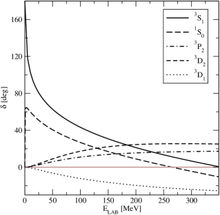
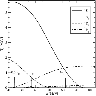
Figure 1: Left panel. Dependence of experimental scattering phase shifts in ${}^{3}S_{1}$, ${}^{3}P_{2}$, ${}^{3}D_{2}$, and ${}^{3}D_{1}$ partial waves on laboratory energy. Right panel. Dependence of critical temperatures of superfluid phase transitions in attractive channels on chemical potential. The corresponding densities are indicated by arrows.

The existence of neutron-star superfluidity, first envisioned by Migdal [11] in 1959, is broadly consistent with microscopic theories of nucleonic matter in NS. Shortly after the advent of the Bardeen-Cooper-Schrieffer (BCS) theory in 1957, BCS pairing of nucleons in nuclei and infinite nuclear matter was suggested and studied.[12, 13] With the discovery of pulsars, the implications of nucleonic pairing for neutron-star properties were explored,[14] and viable microscopic calculations of pairing gaps began to appear soon thereafter.[15, 16, 17, 18, 19]

Partial-wave analysis of the nucleon-nucleon ($NN$) scattering data yields information on the dominant pairing channel in nuclear- and neutron-matter problems in a given range of density (see Fig. 1). At high densities, corresponding to laboratory energies above 250 MeV, the most attractive pairing channel is the tensor-coupled ${}^{3}P_{2}$–${}^{3}F_{2}$ channel,[20, 21] whenever isospin symmetry is even slightly broken. This condition holds inside neutron stars, with the partial densities of neutron and proton fluids differing quite significantly, except in special meson-condensed phases where the nucleonic matter is isospin-symmetric. In such a case the phase-shift analysis predicts that the most attractive pairing interaction is in the ${}^{3}D_{2}$ wave.[22, 23]

At low density, isospin-symmetric nuclear matter exhibits pairing due to the attractive interaction in the ${}^{3}S_{1}$–${}^{3}D_{1}$ partial wave, a tensor component of the force again being responsible for the coupling of the $S$ and $D$ waves.[24, 25, 26, 27] This interaction channel is distinguished by its ability to support a two-body bound state in free space – the deuteron. However, under the highly isospin-asymmetric condition typical in neutron stars, neutron-proton pair condensation is quenched by the large discrepancy between the neutron and proton Fermi momenta (see Sec. 3).

This review is devoted to several aspects of nucleonic superfluidity in neutron stars that are of major current interest. Section 2 provides an overview of the many-body theories of pairing in neutron stars, with a special focus on the Green’s function description of pairing, and the effects of self-energies and vertex corrections. The key ideas of the correlated-basis (or “CBF”) approach to superfluid states of Fermi systems are also presented. Section 3 is concerned with the possibility of pairing between particles lying on different Fermi surfaces, in particular, between protons and neutrons in asymmetric nuclear matter. Here we determine the critical value of isospin asymmetry at which a transition from ${}^{3}S_{1}$–${}^{3}D_{1}$ to ${}^{1}S_{0}$ pairing occurs. (This threshold value is small compared to $p-n$ asymmetries typical of neutron-star matter). More generally, we consider several competing phases that could exist in asymmetric mixtures of fermion species. There exist systems of this kind, notably dilute, ultracold atomic gases and baryonic matter as described by QCD at high density, where “asymmetric pairing” is enforced. (In the case of dilute atomic gases, such conditions can be “tuned in” by external fields, while in the QCD problem, the conditions of charge neutrality and $\beta$ equilibrium together with the heaviness of the strange quark lead naturally to asymmetric pairing among light quarks.) In Sec. 4 we turn to the phenomenon of crossover from BCS superconductivity to Bose-Einstein condensation, as it occurs in fermionic systems that support a two-body bound state in free space. Section 5 is devoted to the physics of superfluids at the “mesoscopic” scale, with discussions of flux quantization, neutron vorticity, the electrodynamics of superconducting protons, and their implications for modeling the dynamics of rotational anomalies in pulsar timing. Our conclusions and related perspectives are summarized in Sec. 6. Two other recent reviews[28, 29] offer complementary information and perspectives on nuclear pairing and nucleonic superfluidity.

2 Many-body theories of pairing

1 Propagators

This subsection outlines the Green’s functions method for the treatment of superfluid systems. The original formulations of this approach are due to Gor’kov and Nambu, who employed thermodynamic Green’s functions.[30] Herein we consider the real-time, finite-temperature formalism, which is suited to studies of both equilibrium and non-equilibrium systems. Our discussion is restricted to equilibrium systems, and we shall work with the retarded components of the full Green’s function of the non-equilibrium theory. Superfluid systems are described in terms of $2\times 2$ matrices of propagators (known as Nambu-Gor’kov matrix propagators) that are defined as

$${\cal G}_{\alpha\beta}(x,x^{\prime}) = \left(\begin{array}[]{cc}G_{\alpha\beta}(x,x^{\prime})&F_{\alpha\beta}(x,x^{\prime})\\ -F^{\dagger}_{\alpha\beta}(x,x^{\prime})&\tilde{G}_{\alpha\beta}(x,x^{\prime})\\ \end{array}\right)$$ (3)

$$= \left(\begin{array}[]{cc}-i\langle T\psi_{\alpha}(x)\psi_{\beta}^{\dagger}(x^{\prime})\rangle&\langle T\psi_{\alpha}(x)\psi_{\beta}(x^{\prime})\rangle\\ \langle T\psi_{\alpha}^{\dagger}(x)\psi_{\beta}^{\dagger}(x^{\prime})\rangle&-i\langle T\psi^{\dagger}_{\alpha}(x)\psi_{\beta}(x^{\prime})\rangle\end{array}\right)\,,$$ (6)

where $\psi_{\alpha}(x)$ are the baryon field operators, $x$ is the space-time coordinate, the indices $\alpha$ and $\beta$ stand for the internal (discrete) degrees of freedom, and $T$ and $\tilde{T}$ denote time-ordering and inverse time-ordering of operators, respectively. The $2\times 2$ matrix Green’s function (3) satisfies the Schwinger-Dyson equation

$${\cal G}_{\alpha\beta}(x,x^{\prime})={\cal G}^{0}_{\alpha\beta}(x,x^{\prime})+\sum_{\gamma,\delta}\!\int\!\!d^{4}x^{\prime\prime}d^{4}x^{\prime\prime\prime}{\cal G}^{0}_{\alpha\gamma}(x,x^{\prime\prime\prime}){\Omega}_{\gamma\delta}(x^{\prime\prime\prime},x^{\prime\prime}){\cal G}_{\delta\beta}(x^{\prime\prime},x^{\prime}),$$ (7)

where the free-propagator matrices ${\cal G}^{0}_{\alpha\beta}(x,x^{\prime})$ are diagonal in the Nambu-Gor’kov space. The matrix structure of the self-energy $\Omega_{\alpha\beta}(x,x^{\prime})$ is identical to that of the propagators: the on-diagonal elements are $\Sigma(p)$ and $\Sigma(-p)$, and the off-diagonal elements are $\Delta(p)$ and $\Delta^{\dagger}(p)$. Fourier transforming Eq. (7) with respect to the relative coordinate $x-x^{\prime}$, one obtains the Dyson equation in the momentum representation. In this representation, the components of the Nambu-Gor’kov matrix obey the coupled Dyson equations

$${G}_{\alpha\beta}(p) = {G}_{0\alpha\beta}(p)+{G}_{0\alpha\gamma}(p)\left[{\Sigma}_{\gamma\delta}(p){G}_{\delta\beta}(p)+{\Delta}_{\gamma\delta}(p){F^{\dagger}}_{\delta\beta}(p)\right]\,,$$ (8)

$${F^{\dagger}}_{\alpha\beta}(p) = {G}_{0\alpha\gamma}(-p)\left[{\Delta}^{\dagger}_{\gamma\delta}(p){G}_{\delta\beta}(p)+{\Sigma}_{\gamma\delta}(-p){F^{\dagger}}_{\delta\beta}(p)\right]\,.$$ (9)

Here ${G}_{\alpha\beta}(p)$ and ${G}_{0\alpha\beta}(p)$ are the full and free normal propagators, ${F^{\dagger}}_{\alpha\beta}(p)$ and ${F}_{\alpha\beta}(p)$ are the anomalous propagators, and ${\Sigma}_{\alpha\beta}(p)$ and ${\Delta}_{\alpha\beta}(p)$ are the normal and anomalous self-energies. The Greek subscripts are the spin/isospin indices, and summation over repeated indices is understood. For systems with time-reversal symmetry, it is sufficient to solve Eqs. (8) and (9), since this symmetry implies that $\Delta_{\alpha\beta}(p)=[\Delta^{\dagger}_{\alpha\beta}(p)]^{*}.$ It is instructive to rewrite Eqs. (8)–(9) in terms of auxiliary Green’s functions

$$G^{N}_{\alpha\beta}(p) = G_{0\alpha\beta}(p)+G^{N}_{\alpha\gamma}(p)\Sigma_{\gamma\delta}(p)G_{0\delta\beta}(p)$$ (10)

describing the unpaired state. The solution of this equation is $G^{N}_{\alpha\beta}(p)=\delta_{\alpha\beta}[\omega-\varepsilon(p)]^{-1}$, where $\varepsilon(p)=\epsilon_{p}+\Sigma(p)$ and $\epsilon_{p}$ is the free single-particle spectrum. (N.B. Assuming that the forces conserve spin and isospin, the self-energy $\Sigma(p)$ is diagonal in spin and isospin spaces). Combining Eqs. (8), (9), and (10), we derive an alternative but equivalent form of the Schwinger-Dyson equations, namely

$$G_{\alpha\beta}(p)=G^{N}_{\alpha\gamma}(p)\left[\delta_{\gamma\beta}+\Delta_{\gamma\delta}(p)F^{\dagger}_{\delta\beta}(p)\right],\quad F^{\dagger}_{\alpha\beta}(p)=G^{N}_{\alpha\gamma}(-p)\Delta^{\dagger}_{\gamma\delta}(p)G_{\delta\beta}(p)\,,$$

which can be solved to obtain

$$G_{\alpha\beta}(p) = \delta_{\alpha\beta}\frac{\omega-E_{A}(p)+E_{S}(p)}{\left[\omega-E_{A}(p)\right]^{2}-E_{S}(p)^{2}-\Delta^{2}(p)}\,,$$ (11)

$$F^{\dagger}_{\alpha\beta}(p) = \frac{\Delta^{\dagger}_{\alpha\beta}(p)}{\left[\omega-E_{A}(p)\right]^{2}-E_{S}(p)^{2}-\Delta^{2}(p)}\,.$$ (12)

Here we have made the substitution $\Delta(p)\Delta^{\dagger}(p)=-\Delta^{2}(p)$ and defined symmetric and antisymmetric parts of the single-particle spectrum in the normal state, $E_{S/A}=\left[\varepsilon(p)\pm\varepsilon(-p)\right]/2.$ For isotropic systems, the self-energy is invariant under reflections in space (i.e. the self-energy is even under $\bm{p}\to-\bm{p})$; furthermore, for systems that are time-reversal invariant, the self-energies are even under the transformation $\omega\to-\omega$. Hence the antisymmetric piece of the spectrum $E_{A}$ must be absent when both conditions are met. The poles of the propagators (11) determine the excitation spectrum of the superfluid system, given by

$$\omega_{\pm}=E_{A}(p)\pm\sqrt{E_{S}(p)^{2}+\Delta^{2}(p)}\,.$$ (13)

Here one sees that there is a finite energy cost $\sim 2\Delta$ for creating an excitation from the ground state of the system when $E_{A}=0$, a property that leads to the existence of superflow or supercurrent in paired fermionic systems.

The solutions (11) and (12) are completely general, all functions being dependent on the three-momentum and the energy. Superfluid systems are often treated in the quasiparticle approximation, in which the self-energies are approximated by their on-mass-shell counterparts. The rationale behind such an approach is that the nuclear system in its ground state can then be described in terms of Fermi-liquid theory, if one neglects pair correlations. Switching on the pair correlations precipitates a rearrangement of the Fermi-surface, but it is assumed that the quasiparticle concept remains intact.

Within this framework, the wave-function renormalization is defined by expanding the normal self-energy as $\Sigma(\omega)=\Sigma(\varepsilon_{p})+\partial_{\omega}\Sigma(\omega)|_{\omega=\varepsilon_{p}}(\omega-\varepsilon_{p})$, where $\varepsilon_{p}=\epsilon_{p}+{\rm Re}\,\Sigma(\varepsilon_{p})$ is the on-mass-shell single-particle spectrum in the normal state that solves Eq. (10). Now, it is seen that the propagators (11) and (12) retain their form if they are renormalized as

$$\tilde{G}(p)=Z(\bm{p})G(\omega+i\delta,\bm{p}),\quad\tilde{F}^{\dagger}(p)=Z(\bm{p})F^{\dagger}(\omega+i\delta,\bm{p}),\quad\tilde{\Delta}^{2}(p)=Z(\bm{p})^{2}\Delta^{2}(\bm{p})\,,$$ (14)

where $Z(\bm{p})\equiv\left[1-\partial_{\omega}\Sigma(\omega)|_{\omega=\varepsilon_{p}}\right]^{-1}$ is the wave-function renormalization and the tilde identifies renormalized quantities. An additional feature of the renormalized propagators is that the quasiparticle spectrum $\varepsilon(p)$ is now constrained to the mass shell. (N.B. For time-local interactions the gap function is energy-independent, so there is no need to expand $\Delta(\omega)$ around its on-shell value. We shall return to the off-shellness of the self-energies in Subsec. 4.)

Renormalization of propagators within the quasiparticle picture suggests that the probability of finding an excitation with given momentum $\bm{p}$ is strongly peaked at the value $\varepsilon_{p}$. The wave-function renormalization takes into account corrections that are linear in the departure from this value. From the computational point of view, such corrections require a knowledge of the off-shell normal self-energies. The dependence of the imaginary part of the self-energy (quasiparticle damping) on frequency follows from Fermi-liquid theory, being given by $2\,{\rm Im}\Sigma(\omega)=a\left[1+\left({\omega}/{2\pi T}\right)^{2}\right]$, where $a$ is a density-dependent constant. The real part of the self-energy, ${\rm Re}\Sigma(\omega)$, can be computed from ${\rm Im}\Sigma(\omega)$ via the Kramers-Kronig dispersion relation only if the latter function is known for all frequencies $\omega\in[-\infty,\infty]$. Accordingly, the foregoing result from Fermi-liquid theory should be supplemented by a model of the high-energy tail of the quasiparticle damping.

The momentum dependence of propagators can be approximated by introducing an effective quasiparticle mass. For nonrelativistic particles, expansion of the normal self-energy around the Fermi momentum leads to

$$\varepsilon(p)=\frac{p_{F}}{m^{*}}(p-p_{F})-\mu^{*}\,,\quad\quad\frac{m^{*}}{m}=\left[1+\frac{m}{p_{F}}\partial_{p}\mathop{\rm Re}\Sigma(p)|_{p=p_{F}}\right]^{-1}\,.$$ (15)

where $\mu^{*}\equiv-\epsilon(p_{F})+\mu-\mathop{\rm Re}\Sigma(p_{F})$. A closed system of equations determining the properties of the superfluid system is obtained by specifying the self-energies in terms of the propagators and interactions, as discussed below.

2 Mean-field BCS theory

The BCS-type theory of superconductivity as applied to nuclear systems is predicated on a mean-field approximation to the anomalous self-energy. Specifically, the anomalous self-energy is expressed through the four-point vertex function $\Gamma(p,p^{\prime})$ in the form

$$\Delta(p)=-2\int\!\frac{d^{4}p^{\prime}}{(2\pi)^{4}}\Gamma(p,p^{\prime})\,{\rm Im}F(p^{\prime})f(\omega^{\prime})\,,$$ (16)

where $f(\omega)=[1+{\rm exp}(\beta\omega)]^{-1}$ and $\beta$ is the inverse temperature. We observe that the gap is energy-independent when the interactions are local in time, corresponding to no retardation, as in the case where the effective interaction $\Gamma(p,p^{\prime})$ is replaced by the bare interaction $V(\bm{p},\bm{p}^{\prime})$. In this case, carrying out the renormalization according to Eq. (14) and integrating over the energy, we arrive at[31, 32, 33]

$$\tilde{\Delta}(\bm{p})=Z(\bm{p})\int\!\frac{d^{3}p^{\prime}}{2(2\pi)^{3}}V(\bm{p},\bm{p}^{\prime})Z(\bm{p}^{\prime})\frac{\tilde{\Delta}(\bm{p}^{\prime})}{\tilde{\omega}_{+}(\bm{p}^{\prime})}\left[f(\omega_{+})-f(\omega_{-})\right]\,,$$ (17)

where $\tilde{\omega}_{\pm}=\pm\sqrt{\varepsilon_{p}^{2}+\tilde{\Delta}^{2}}$ [cf. Eq. (13)]. Further progress requires partial-wave decomposition of the interaction in Eq. (17). To avoid excessive notation, our consideration focuses on a single, uncoupled channel, for which we obtain a one-dimensional gap equation

$$\tilde{\Delta}(p)=Z(p)\int\frac{dp\,p^{2}}{(2\pi)^{2}}V(p,p^{\prime})Z(p^{\prime})\frac{\tilde{\Delta}(p^{\prime})}{\tilde{\omega}_{+}(p^{\prime})}\left[f(\tilde{\omega}_{+})-f(\tilde{\omega}_{-})\right]\,,$$ (18)

where $V(p,p^{\prime})$ is the interaction in the given partial wave. The gap equation is supplemented by the equation for the density of the system,

$$\rho=-2g\int\!\!\frac{d^{4}p}{(2\pi)^{4}}{\rm Im}G(p)f(\omega)=\frac{g}{2}\int\!\!\frac{d^{3}p}{(2\pi)^{3}}Z(\bm{p})\sum_{i=+,-}\left(1+\frac{\varepsilon_{p}}{\tilde{\omega}_{i}}\right)f(\tilde{\omega}_{i})\,,$$ (19)

which determines the chemical potential in a self-consistent manner. Here $g$ is the isospin degeneracy factor. Eqs. (16)–(19) define mean-field BCS theory. In subsequent discussions based on this theory, the tilde notation will be suppressed.

Assuming that the interaction $V(p,p^{\prime})$ and the single-particle spectrum $\varepsilon_{p}$ in the unpaired state are known, Eqs. (18) and (19) form a closed system for the gap and chemical potential. Within this formulation, the presence of a hard core in the interaction causes no overt problems, for one can readily show that at the critical temperature, Eq. (18) transforms into an integral equation that sums the particle-particle ladder series to all orders. In the special case in which the interaction is momentum-independent, Eq. (18) leads to the familiar weak-coupling formula

$$\Delta(p_{F})\simeq 8\mu^{*}\,{\rm exp}\left(-\frac{1}{\nu(p_{F})|V(p_{F},p_{F})|}\right)\,,$$ (20)

where the density of states is specified by $\nu(p_{F})=m^{*}p_{F}Z^{2}(p_{F})/2\pi^{2}$ (for one direction of isospin). The weak-coupling formula is often used to estimate the magnitude of the gap. However, because realistic pairing interactions are momentum-dependent, the density dependence of the gap predicted by Eq. (18) may deviate markedly from that given by the weak-coupling formula (20). Moreover, as argued in Ref. KKC, if the pairing interaction acquires a strong momentum dependence due to a short-range repulsive core, the weak-coupling formula may well produce a meaningless or useless estimate of the gap, since its derivation requires that $V(p,p^{\prime})$ take a negative value on the Fermi surface.

The normal-state self-energy is written as

$$\Sigma(p)=-2\int\frac{d^{4}p^{\prime}}{(2\pi)^{4}}T\left(p,p^{\prime};p+p^{\prime}\right)_{A}{\rm Im}G(p^{\prime})f(\omega^{\prime})\,,$$ (21)

where the subscript $A$ indicates antisymmetrization of the final states and the contribution $\propto{\rm Im}T$ is omitted for simplicity. For nuclear systems, the amplitude $T$ is often approximated by the scattering $T$-matrix, which sums up the ladder diagrams and is generally nonlocal.

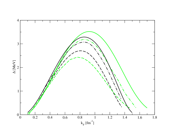
Figure 2: Singlet $S$-wave (${}^{1}S_{0}$) pairing gap in neutron matter and nuclear matter versus Fermi momentum. The heavy and light lines correspond respectively to the phase-shift-equivalent Nijmegen interaction and the Gogny effective interaction DS1. Solid lines and dashed-dotted lines label results for pure neutron matter using the free-space single-particle spectrum and implementing single-particle renormalization, respectively, while the dashed line refers to symmetrical nuclear matter with single-particle renormalization.

An alternative is to replace the $T$-matrix by an effective time-local interaction that is fitted to properties of finite nuclei (e.g. a Skyrme or Gogny force), in which case Eq. (21) reduces to a mean-field Hartree-Fock approximation. However, one must be aware that the normal-state spectrum itself must depend on the anomalous self-energy $\Delta(p)$. The common replacement of $G(p)$ by $G^{N}(p)$ when computing the normal-state spectrum is an approximation (sometimes called the “decoupling approximation”), which is justified when the pairing effects can be viewed as a perturbation to the normal state, but must be made with care.

Fig. 2 shows the ${}^{1}S_{0}$ pairing gap in neutron matter and symmetrical nuclear matter for the high-precision phase-shift-equivalent Nijmegen potential and the effective Gogny DS1 force, for different approximations to the single-particle spectrum.[35] In the case of smooth effective forces such as the the Gogny interaction, a Hartree-Fock approximation to the normal self-energy is suitable and was adopted; for the (realistic) Nijmegen potential, the $T$-matrix was calculated in Brueckner theory. In both cases, the full momentum-dependent self-energies Re$\Sigma(\bm{p})$ were used in the gap equation. The momentum renormalization yields an effective mass $m^{*}/m$ less than unity, thus reducing the density of states $\nu(p_{F})$ on the Fermi surface and hence also reducing the size of the gap. The wave-function renormalization factor $Z(\bm{p})$ is also less than one, leading to an additional suppression of the gap. However, the the magnitude of this effect is yet to be established.[32, 33]

3 Polarization effects

An improvement upon the mean-field BCS approximation to fermion pairing is achieved in theories that take into account the modifications of the pairing interaction due to the background medium. In diagrammatic language, the class of modifications known as “polarization effects” or “screening” arise from the particle-hole bubble diagrams, ideally summed to all orders starting from the bare interaction as the driving term. Consider the following integral equation describing the four-fermion scattering process $p_{1}+p_{2}\to p_{3}+p_{4}$:

$$\Gamma(p,p^{\prime},q)=U(p,p^{\prime},q)-i\int\!\frac{d^{4}p^{\prime\prime}}{2\pi)^{4}}\,U(p,p^{\prime\prime},q)G^{N}(p^{\prime\prime}+q/2)G^{N}(p^{\prime\prime}-q/2)\Gamma(p^{\prime\prime},p^{\prime},q)\,,$$ (22)

where $q=p_{1}-p_{2}$ is the momentum transfer, $p=p_{1}+p_{3}$, and $p^{\prime}=p_{2}+p_{4}$. Eq. (22) sums the particle-hole diagrams to all orders. To avoid double summation in the gap equation, the driving term $U(p,p^{\prime},q)$ must be devoid of blocks that contain particle-particle ladders. This driving interaction depends in general on the spin and isospin and can be decomposed as

$$U_{\bm{q}}=f_{\bm{q}}+g_{\bm{q}}(\bm{\sigma}\cdot\bm{\sigma}^{\prime})+\left[f^{\prime}_{\bm{q}}+g^{\prime}_{\bm{q}}(\bm{\sigma}\cdot\bm{\sigma}^{\prime})\right](\bm{\tau}\cdot\bm{\tau}^{\prime})\,,$$ (23)

where $\bm{\sigma}$ and $\bm{\tau}$ are the vectors formed from the Pauli matrices in the spin and isospin spaces. We assume here that the interaction block $U$ depends only on the momentum transfer. For illustrative purposes, the tensor part of the interaction and the spin-orbit terms are ignored. (However, see Subsec. 4, where the tensor component is included by means of pion exchange.) Solution of the integral equation (22) then takes the form

$$\nu(p_{F})\Gamma_{\bm{q}} = \frac{F_{\bm{q}}}{1+\Lambda(q)F_{\bm{q}}}+\frac{G_{\bm{q}}}{1+\Lambda(q)G_{\bm{q}}}(\bm{\sigma}\cdot\bm{\sigma}^{\prime})$$ (24)

$$+ \left[\frac{F^{\prime}_{\bm{q}}}{1+\Lambda(q)F^{\prime}_{\bm{q}}}+\frac{G^{\prime}_{\bm{q}}}{1+\Lambda(q)G^{\prime}_{\bm{q}}}(\bm{\sigma}\cdot\bm{\sigma}^{\prime})\right](\bm{\tau}\cdot\bm{\tau}^{\prime})\,,$$

where $F_{\bm{q}}=\nu(p_{F})f_{\bm{q}}$, $G_{\bm{q}}=\nu(p_{F})g_{\bm{q}}$, $F^{\prime}_{\bm{q}}=\nu(p_{F})f^{\prime}_{\bm{q}}$, and $G^{\prime}_{\bm{q}}=\nu(p_{F})g^{\prime}_{\bm{q}}$ , while

$$\Lambda(q)=\nu(p_{F})^{-1}\int\!\frac{d^{4}p^{\prime\prime}}{(2\pi)^{4}}\,G^{N}(p^{\prime\prime}+q/2)G^{N}(p^{\prime\prime}-q/2)\,,$$ (25)

is the (dimensionless) Lindhard function (or polarization tensor). We are tacitly assuming that the system is in a state characterized by a well-defined Fermi sphere. Then, if the momenta of both particles lie on the Fermi surface, the momentum transfer is related to the scattering angle via $q=2p_{F}\sin\theta/2$, and the parameters $F$, $F^{\prime}$, $G$, and $G^{\prime}$ can be expanded in spherical harmonics with respect to the scattering angle, according to

$$\left(\begin{array}[]{c}F(q)\\ G(q)\end{array}\right)=\sum_{l}\left(\begin{array}[]{c}F_{l}\\ G_{l}\end{array}\right)P_{l}(\cos\theta)\,,$$ (26)

and similarly for $F^{\prime}(q)$ and $G^{\prime}(q)$. The Landau parameters $F_{l}$, $G_{l}$, $F_{l}^{\prime}$, and $G_{l}^{\prime}$ depend only on the density. The isospin degeneracy of neutron matter, reflected in $\bm{\tau}\cdot\bm{\tau}^{\prime}=1$, implies that the number of independent Landau parameters for each $\bf q$ or $l$ reduces from four to two, defined by $F^{n}=F+F^{\prime}$ and $G^{n}=G+G^{\prime}$. Commonly, only the lowest-order harmonics in the expansion (26) are needed. For a singlet pairing state, in which the total spin of the pair is $S=0$ and $\bm{\sigma}\cdot\bm{\sigma}^{\prime}=-3$, the pairing interaction is given by

$$\nu(p_{F})\Gamma_{q}=F_{0}^{n}\left[1-\frac{\Lambda(q)F_{0}^{n}}{1+\Lambda(q)F_{0}^{n}}\right]-3G_{0}^{n}\left[1-\frac{\Lambda(q)G_{0}^{n}}{1+\Lambda(q)G_{0}^{n}}\right]\,.$$ (27)

In general, the polarization tensor $\Lambda(q)$ is complex-valued. However, in the limit of zero energy transfer (at fixed momentum), it is real and becomes simply

$$\Lambda(q)=-1+\frac{p_{F}}{q}\left(1-\frac{q^{2}}{4p_{F}^{2}}\right){\rm ln}\Bigg{|}\frac{2p_{F}-q}{2p_{F}+q}\Bigg{|}\,$$ (28)

in the zero-temperature limit. Eq. (27) contains two distinct contributions: the direct part generated by the terms 1 inside the square brackets, and the remaining, induced part that accounts for density and spin-density fluctuations. If the Landau parameters are known – either by inferring them from experiment or by computing them within an ab initio many-body scheme – the effect of polarization can be assessed by defining an averaged interaction

$$\Gamma=\frac{1}{2p_{F}^{2}}\int_{0}^{2p_{F}}dq\,q\Gamma(q)\,.$$ (29)

The effect of density fluctuations $\propto F^{n}_{0}$ is to enhance the attraction in the pairing interaction[36] and therefore increase the gap, while the spin-density fluctuations $\propto G^{n}_{0}$ tend to reduce the attraction and decrease the gap.[37] At densities typical of the inner crust of a neutron star, the values of microscopically derived Landau parameters imply that the suppression of pairing via spin-density fluctuations is the dominant effect.[37] The Landau parameters of neutron matter and symmetrical nuclear matter have been studied extensively within complex many-body schemes[38, 39, 40] whose description is beyond the scope of this chapter. It should be noted, however, that the matrix elements of the pairing interactions derived in some of these schemes, including the Babu-Brown approach[38, 39] and its extensions such as polarization-potential theory, [41, 42] have been used in conjunction with the weak-coupling approximation (20), which – as indicated above – is generally inadequate in the nuclear/neutron-matter context.

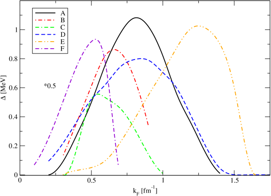
Figure 3: Singlet $S$-wave (${}^{1}S_{0}$) pairing gaps in neutron matter versus Fermi momentum, as obtained from microscopic calculations that attempt to account for medium-modification of the pairing interaction and self-energies. The curves are labeled as: A - Wambach et al. [42], B - Chen et al. [48], C - Chen et al. [49], D - Schwenk et al. [52], E - Schulze et al. [51], F - Fabrocini et al. [50].

The initial microscopic calculations of the effects of medium polarization on pairing were carried out within an alternative many-body approach, the method of Correlated Basis Functions (CBF)[43, 44, 45, 46, 47, 48, 49] (to be described in Subsec. 5). At a qualitative level, the findings of the CBF studies of Chen et al.[48, 49] are consistent with much of the later work based on Green’s functions and Fermi-liquid theories. Until recently, there was broad agreement that the screening reduces the singlet $S$-wave gap by factor of 3 or so (c.f. Fig. 2). However, the density profiles of the calculated gaps differ considerably. This is illustrated in Fig. 3, which presents a composite plot of theoretical predictions for the dependence of the ${}^{1}S_{0}$ pairing gap at the Fermi surface, $\Delta(k_{F})$, upon the Fermi wave number $k_{F}=p_{F}/\hbar=(3\pi^{2}\rho)^{1/3}$. The six curves in the plot correspond to various microscopic approaches that include a screening correction. The results of Wambach et al.,[42] Schulze et al.,[51] and Schwenk et al.[52] are based on microscopic treatments rooted in Landau/Fermi-liquid theory, with polarization-type diagrams summed to all orders. The results of Chen et al.[48, 49] and Fabrocini et al.[50] were obtained within two different implementations of CBF theory.

Further assessment of the status of quantitative microscopic evaluation of the singlet-$S$ gap is deferred until Subsec. 5, where the elements of CBF approaches to the pairing problem are reviewed. We may already remark, however, that explicit comparison of the pairing matrices constructed in the different theories could help to eliminate discrepancies introduced by use of the weak-coupling approximation in some of the theoretical treatments. Another important consideration is consistent inclusion of medium effects on both the pairing interaction and the self-energies.

4 Non-adiabatic superconductivity

Since mesons propagate in nuclear matter at finite speed, the interactions among nucleons are necessarily retarded in character. As a consequence, the self-energies (and in particular the gap function) must depend on energy or frequency. Within the meson-exchange picture of nuclear interactions, the lightest mesons – pions – should be the main source of nonlocality in time. This suggests that it may be fruitful to consider a pairing model in which the interactions are modeled in terms of pion exchanges, plus contact terms that can be approximated by Landau parameters. Thus one assumes an interaction structure

$$V_{NN}=-\frac{f_{\pi}}{m_{\pi}}(\bm{\sigma}\cdot\bm{\nabla})(\bm{\tau}\cdot\bm{\phi})+\tilde{U}(q)$$ (30)

in which $\bm{\phi}$ is the pseudoscalar isovector pion field satisfying the Klein-Gordon equation, $f_{\pi}$ is the pion-nucleon coupling constant, and $m_{\pi}$ is the pion mass. Here $\bm{\phi}$ is the pseudoscalar isovector pion field satisfying the Klein-Gordon equation, $f_{\pi}$ is the pion-nucleon coupling constant, and $m_{\pi}$ is the pion mass. The operator structure of the term $\tilde{U}(q)$ is like that of Eq. (23), but with constants differing numerically since the tensor one-pion exchange is treated separately.

For static pions, the one-pion-exchange two-nucleon interaction in momentum space is given by

$$V_{\pi}(\bm{q})=-\frac{f_{\pi}^{2}}{3m_{\pi}^{2}}\,\frac{\bm{q}^{2}}{\bm{q}^{2}+m_{\pi}^{2}}\left[\bm{\sigma}_{1}\cdot\bm{\sigma}_{2}+S_{12}(\bm{n})\right]\bm{\tau}_{1}\cdot\bm{\tau}_{2}\,,$$ (31)

where $\bm{q}$ is the momentum transfer, $\bm{n}=\bm{q}/q$, and $S_{12}(\bm{n})$ is the tensor operator. This interaction is known to reproduce the low-energy phase shifts and, to a large extent, the deuteron properties.[53] Below, however, the pairing correlations are evaluated from the diagrams that contain dynamical pions, with full account of the frequency dependence of the pion propagators. The static results can be recovered, and a relation to the phase shifts established, only in the limit $\omega\to 0$ in the pion propagator. The dynamics at intermediate and short range is dominated in turn by the correlated two-pion, $\rho$-meson, and heavier-meson exchanges. Short-range correlations are crucial for a realistic description of low-energy phenomena, being necessary to achieve nuclear saturation. Moreover, the response functions calculated from one-pion exchange alone would already precipitate a pion-condensation instability in nuclear matter at an unrealistically low density.

The interaction (30) leads to a time-nonlocal formulation of nuclear superconductivity in neutron-star matter.[54] The Dyson-Schwinger equation (7) provides the starting point. Since the formulation will incorporate the full frequency dependence of the self-energies, it is useful (and also conventional [55]) to define the wave-function renormalization differently than in Subsec. 2. Thus we set $Z(p)=1-\omega^{-1}\Sigma_{A}(p)$, the retarded self-energy being decomposed into components even ($S$) and odd ($A$) in $\omega$, i.e. $\Sigma(p)=\Sigma_{S}(p)+\Sigma_{A}(p)$. The single-particle energy is then renormalized as $E_{S}=\epsilon_{p}+\Sigma_{S}(E_{S},\bm{p})$. Accordingly, the propagators now take the forms

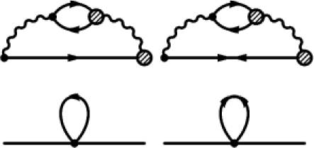
Figure 4: Top panel. Baryon Fock-exchange self-energies for normal (left graph) and anomalous (right graph) sectors. The solid lines correspond to fermions; and the wavy lines, to pions. The blobs symbolize RPA-renormalized vertices; and the dots, bare pion-nucleon vertices. Bottom panel. Normal and anomalous Hartree diagrams. The dots stand for contact Landau interactions; the straight lines are shown for clarity.

$$G(p) = \frac{\omega Z(p)+E_{S}(p)}{(\omega+i\eta)^{2}Z(p)^{2}-E_{S}(p)^{2}-\Delta(p)^{2}}\,,$$ (32)

$$F(p) = -\frac{\Delta(p)}{(\omega+i\eta)^{2}Z(p)^{2}-E_{S}(p)^{2}-\Delta(p)^{2}}\,,$$ (33)

where $\Delta\Delta^{\dagger}\equiv-\Delta^{2}$. The self-energies of the theory are shown in Fig. 4. The analytical counterparts of the Fock self-energies are

$$\Sigma^{\rm Fock}(\omega,\bm{p}) = -2\int\!\!\frac{d^{3}q}{(2\pi)^{3}}\int_{-\infty}^{\infty}\!\!\frac{d\varepsilon}{2\pi}\Xi_{0}(\bm{q}){\rm Im}G(\varepsilon,\bm{p}-\bm{q})C(\omega,\varepsilon,\bm{q})\Xi(\bm{q})\,,$$ (34)

$$\Delta^{\rm Fock}(\omega,\bm{p}) = -2\int\!\!\frac{d^{3}q}{(2\pi)^{3}}\int_{-\infty}^{\infty}\!\!\frac{d\varepsilon}{2\pi}\Xi_{0}(\bm{q}){\rm Im}F(\varepsilon,\bm{p}-\bm{q})C(\omega,\varepsilon,\bm{q})\Xi(\bm{q})\,,$$ (35)

where

$$C(\omega,\varepsilon,\bm{q})=\int_{0}^{\infty}\!\!\frac{d\omega^{\prime}}{2\pi}B(\omega^{\prime},\bm{q})\left[\frac{f(\varepsilon)+g(\omega^{\prime})}{\varepsilon-\omega^{\prime}-\omega-i\eta}+\frac{1-f(\varepsilon)+g(\omega^{\prime})}{\varepsilon+\omega^{\prime}-\omega-i\eta}\right]\,.$$ (36)

Here $B(q)$ is the pion spectral function, while $\Xi^{0}(q)$ and $\Xi(q)$ are the bare and renormalized pion-neutron vertices. One remarkable feature of Eqs. (34)–(36) is that the energy and momentum dependence of the self-energies is determined by the dynamical features of the meson (here pion) field. Another salient feature is that the normal and anomalous sectors are coupled, in contrast to the BCS case, where the unpaired single-particle energy is unaffected by the pairing. The most important contribution to the pion spectral function comes from the coupling to virtual particle-hole states, which are described by the (retarded) particle-hole polarization tensor $\Pi(\omega,\bm{p})$. Specifically, one finds

$$B(q)=\frac{-2{\rm Im}\Pi^{R}(q)}{[\omega^{2}-\bm{q}^{2}-m_{\pi}^{2}-{\rm Re}\Pi^{R}(q)]^{2}+[{\rm Im}\Pi^{R}(q)]^{2}}\,.$$ (37)

Figure 5: Pion spectral function in neutron matter as a function of energy and momentum transfer. The density corresponds to $k_{F}=0.55$ fm^-1.

The spectral function of pions in neutron matter is illustrated in Fig. 5 for the momentum transfer range $0\leq q\leq 2k_{F}$, where $k_{F}=0.55$ fm^-1. It is seen that (i) the spectral function has a substantial weight for finite energy transfer, the maximum being determined by the pion dispersion relation $\tilde{\omega}^{2}=\bm{q}^{2}+m_{\pi}^{2}+{\rm Re}\Pi(\tilde{\omega},q)$ and (ii) the spectral function is substantially broadened due to the excitations of particle-hole pairs, which are treated in the random-phase approximation (RPA).[53] In addition to the Fock self-energies we need to include the Hartree contribution, which reduces to

$$\Delta^{\rm BCS}(\omega,\bm{p}) = -2(F^{n}_{0}-3G^{n}_{0})\int\frac{d^{4}p^{\prime}}{(2\pi)^{4}}{\rm Im}\,F(\omega+\omega^{\prime},\bm{p}+\bm{p}^{\prime})\,.$$ (38)

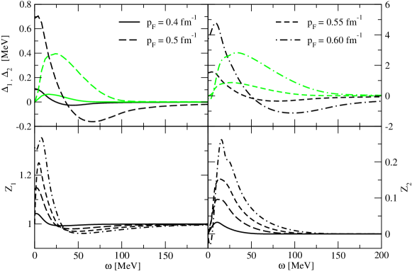
Figure 6: Top panel. Frequency dependence of real (heavy lines) and imaginary (light lines) parts of the gap function, $\Delta_{1}(\omega)$ and $\Delta_{2}(\omega)$, respectively, for $k_{F}=0.4$ (solid), 0.5 (long-dashed), 0.55 (dashed), and 0.6 (dashed-dotted lines) fm^-1. The on-shell values of the pairing gap are 0.1, 0.7, 1.4, and 3.7 MeV for $k_{F}=0.4$, 0.5, 0.55, and 0.6 fm^-1. Bottom panel. Frequency dependence of real (left panel) and imaginary (right panel) parts of the wave-function renormalization, $Z_{1}(\omega)$ and $Z_{2}(\omega)$. Labeling is the same as in the top panel.

Solutions of the self-consistent equations (35) and (36) are shown in Fig. 6 at zero temperature and for densities specified by the indicated Fermi momenta. At small energy transfers, the imaginary components of the gap and wave-function renormalization vanish, and one recovers the BCS limit. For finite energy transfers these functions develop substantial structure that reflects the features of the pion spectral function [the driving term in the kernel of integral equations for $\Delta(q)$ and $Z(q)$]. Note that the actual value of the gap on the mass shell does depend on the detailed structure of these functions far from the mass shell. However, it is possible to renormalize the pion spectral function such that the high-energy tails are eliminated while the on-mass-shell physics is unchanged.

Theories that explicitly include the light mesons – pions or kaons – in the computational scheme have the advantage that they embody the precursor phenomena associated with the softening of the pion (kaon) modes close to the threshold for condensation. In the case of $P$-wave pairing, an enhancement of the pairing correlation has been predicted.[56]

5 The method of correlated basis functions (CBF)

The variational formulation of BCS theory is based on the trial wave function (BCS state)

$$\Psi_{\rm BCS}=\prod_{\bm{p}}\left[(1-h_{\bm{p}})^{1/2}+h_{\bm{p}}^{1/2}\psi^{\dagger}_{{\bm{p}}\uparrow}\psi^{\dagger}_{-{\bm{p}}\downarrow}\right]|0\rangle\,,$$ (39)

where the real function $h_{\bm{p}}$, which gives the occupation probability of the pair state $({\bm{p}}\uparrow,-{\bm{p}}\downarrow)$, is subject to variation. For this trial state one may compute the anomalous density

$$\chi_{\bm{p}}=\langle\Psi_{\rm BCS}|\psi^{\dagger}_{{\bm{p}}\uparrow}\psi^{\dagger}_{-{\bm{p}}\downarrow}|\Psi_{\rm BCS}\rangle=h_{\bm{p}}^{1/2}(1-h_{\bm{p}})^{1/2}\,,$$ (40)

whose Fourier image specifies the spatial structure of a Cooper pair. The standard coupled BCS equations for the energy gap, the fermionic density, and the quasiparticle energy at zero temperature, namely

$$\Delta(p)=-\int\frac{d^{3}p^{\prime}}{(2\pi)^{3}}V(p,p^{\prime})\frac{1}{2E(p^{\prime})}\Delta(p^{\prime})\,,$$ (41)

$$\rho=\int{\frac{d^{3}p}{(2\pi)^{3}}}h_{\bm{p}}=\int\frac{p^{2}dp}{(2\pi)^{2}}\left[1-\frac{\varepsilon(p)-\mu}{2E(p)}\right]\,,$$ (42)

$$E(p)=\sqrt{\left[\varepsilon(p)-\mu\right]^{2}+\Delta^{2}(p)}\,,$$ (43)

are generated naturally upon (i) evaluating the expectation value of the grand-canonical Hamiltonian for the BCS state (39), and (ii) performing a variational minimization of this functional with respect to $h_{\bm{p}}$, under the constraint that the expectation value of the particle-number density coincides with the prescribed density.

Treatment of strongly interacting fermionic systems (including nuclear problems) within a variational framework calls for improved superfluid trial states. The systems of interest are characterized by a bare two-body interaction containing a strong inner repulsive core along with longer-range attractive components. To obtain a reasonable energy expectation value, the trial function must adequately describe the short-range geometric correlations induced by the repulsion, which inhibits the close approach of a pair of particles.[43, 44, 45, 46] The simplest choice involves the Jastrow correlation factor

$$F_{J}=\prod_{i<j}^{N}f(r_{ij})\,,\quad\mathop{\lim}\limits_{r\to 0}f(r)\to 0\,,\quad\mathop{\lim}\limits_{r\to\infty}f(r)\to 1\,,$$ (44)

which is suited to efficient description of state-independent two-body correlations, especially the short-range repulsive effects. As a bonus, with proper optimization of the two-body function $f(r)$, the Jastrow factor can also incorporate effects of virtual phonon excitations and indeed can reproduce the correct asymptotic behavior of long-range correlations.

A substantially improved trial superfluid state of definite particle number may be formed by applying the Jastrow operator (44) to an $N$-particle projection of the BCS trial state, expressed in the configuration-space representation as

$$\Phi^{(N)}_{\rm BCS}=\frac{1}{\sqrt{\cal N}}\,{\cal A}\{\phi(\bm{r}_{1},\bm{r}_{2}),\phi(\bm{r}_{2},\bm{r}_{3})\dots\phi(\bm{r}_{N-1},\bm{r}_{N})\}\,.$$ (45)

Here, $\phi({\bm{r}_{i},\bm{r}_{j}})$ is the antisymmetrized Fourier image of $\chi_{\bm{p}}$ given by Eq. (40), times a spin function, ${\cal A}$ is an antisymmetrization operator acting on particle pairs in different $\phi$ factors, and ${\cal N}$ is a normalization constant. In spirit, this is the approach adopted in the early work of Yang and Clark,[15, 16] although in practice they determined the one-body, two-body, etc. density matrices required for their cluster-expansion treatment of the short-range correlations from the BCS state (39), rather than from its $N$-particle projection (45).

Following up on the work of Refs. YANG1,YANG2, a formal variational theory[58] of the superfluid ground state of uniform, infinite nucleonic systems was developed for a trial correlated BCS state constructed in Fock space,

$$|\Psi_{s}\rangle=\sum_{N}\sum_{m^{(N)}}\hat{F}^{(N)}|\Phi_{m}^{(N)}\rangle\langle\Phi_{m}^{(N)}|{\rm BCS}\rangle\,,$$ (46)

where $\hat{F}^{(N)}$ is an unspecified correlation operator meeting certain minimal conditions and $\{|\Phi_{m}^{(N)}\rangle\}$ is a complete set of Fermi-gas Slater determinants, both referred to the $N$-particle Hilbert space. Thus, the correlated normal states $\{\hat{F}^{(N)}|\Phi_{m}^{(N)}\rangle\}$ are superposed with the same amplitudes as the model states $|\Phi_{m}^{(N)}\rangle$ have in the corresponding grand-canonical representation of the original BCS state (39). Repetition of steps (i) and (ii) above for this correlated superfluid Ansatz yields a theory having the same structure as ordinary BCS theory, when the “decoupling approximation” is applied. In this approximation, only one Cooper pair at a time is considered, while treating the background as normal. Formally, the expectation value of the grand-canonical Hamiltonian is expanded in terms of the deviations of the Bogolyubov amplitudes $u_{\bm{p}}=(1-h_{\bm{p}})^{1/2}$ and $v_{\bm{p}}=h_{\bm{p}}^{1/2}$ about their normal-state values, retaining deviant terms at most of first order in $v_{\bm{p}}^{2}-\theta(p)$ and second order in $u_{\bm{p}}v_{\bm{p}}$, where $\theta(p)$ is the Fermi step.

Within this framework, the gap equation and density constraint maintain the same mean-field forms as obtained for the bare BCS state, except for the attachment of renormalization factors $z_{p}^{-1}$ to the gap function $\Delta(p)$ when it appears in quasiparticle energy denominators. The presence of correlations introduced by the operator ${\hat{F}}^{(N)}$ is otherwise reflected only in the replacement of the pairing matrix elements $V(p,p^{\prime})$ and single-particle energies $\varepsilon(p)$ derived from the bare interaction based on the BCS trial state (39) and variational steps (i)-(ii), by effective pairing matrix elements ${\cal V}(p,p^{\prime})$ and correlation-dressed single-particle energies $\xi(p)$ built from combinations of diagonal and off-diagonal matrix elements of the Hamiltonian and unit operators in the correlated normal bases $\{{\hat{F}}^{(N)}|\Phi_{m}^{(N)}\rangle\}$. When the state-independent Jastrow choice $F_{J}$ of Eq. (44) is assumed for the correlation operator $\hat{F}$, the dressed quantities ${\cal V}(p,p^{\prime})$ and $\xi(p)$ can be evaluated by Fermi hypernetted-chain (FHNC) methods developed in Ref. KRO_CLARKII, with results for neutron matter and liquid ³He reported in Ref. KRO_CLARKIII.

An important advance in the CBF approach to pairing was made in Ref. CBF5, where the variational description was extended to create a correlated-basis perturbation theory for the exact superfluid ground state. Again imposing the decoupling approximation, a sequence of approximations to the grand-canonical energy may be defined, each preserving under variation the standard form of the gap equation, but with successive improvements on the effective pairing matrix elements and dressed self-energies. (A convenient modification of the trial correlated ground state (46) was made by inserting the normalization factor $\langle\Phi_{m}^{(N)}|{F^{(N)}}^{\dagger}F^{(N)}|\Phi_{m}^{(N)}\rangle^{-1/2}$ inside the summations. This eliminates the renormalization factors $z_{p}^{-1}$ mentioned above.) Making the Jastrow choice for the correlation operator $\hat{F}$, the leading perturbative corrections to the variational results for ${\cal V}(p,p^{\prime})$ and $\xi(p)$ were generated, represented in diagrammatic form, and evaluated. These corrections include the leading contribution from medium polarization within the CBF framework. Here we should point out that the terms in the CBF perturbation expansions of the various quantities are not easily interpreted in terms of conventional Goldstone or Feynman diagrams, although they may have similar appearance. A given order in the CBF expansion, including the “zeroth-order” variational term, will contain pieces belonging to any number of perturbative orders in the conventional sense. In general there will be terms accounting for the nonorthogonality of the basis, terms that correct the average-propagator approximation inherent (for example) in the Jastrow description of $\hat{F}$-correlations, terms that correct for non-optimality of the chosen $\hat{F}$-correlations, etc.

In microscopic studies of nucleonic systems, it is generally imperative to include the effects of state-dependent correlations arising from realistic $NN$ interactions which contain, separately in each spin and isospin channel, contributions of central, tensor, and spin-orbit character. In principle, the CBF perturbation expansions provide for systematic correction of the Jastrow Ansatz for the correlation operator $\hat{F}$, so as to incorporate these state-dependent effects. However, it is clearly preferable to take account of state dependence already in the choice of $\hat{F}$, thus reducing the need to correct the variational treatment with CBF perturbation theory. A suitably general correlation Ansatz, within the class containing only two-body correlation factors, is given by

$${\hat{F}}=\prod_{i<j}^{N}f(ij)\,,\qquad f(ij)=\sum_{\alpha=1}^{n}f_{\alpha}(r_{ij})o_{\alpha}(ij)\,,$$ (47)

where $f(ij)$ contains terms for the same operators $o_{\alpha}(ij)$ as are present in the assumed realistic $NN$ interaction (e.g., the Argonne $v_{18}$ model[59]), or an adequate subset of them. Profound difficulties arise in the implementation of this choice, due to non-commutativity among the $o_{\alpha}(ij)$ operators. The analog of FHNC resummation being still beyond our reach for such state-dependent correlations, existing calculations proceed with straightforward cluster or power-series expansions, perhaps with vertex corrections.[49, 50] It is important to appreciate that the extended Jastrow form (47) of the $\hat{F}$-operator is equipped to include the lion’s share of the polarization corrections (just as the simple state-independent Jastrow form is capable of capturing the major effects of density-density fluctuations).

Chen et al.[48] applied CBF pairing theory as developed in Ref. CBF5 to superfluid neutron matter in the ${}^{1}S_{0}$ phase, assuming state-independent Jastrow correlations and taking account of the leading CBF perturbation corrections to the variational treatment. The polarization and other corrections produced a very substantial suppression from the variational estimate of the gap $\Delta(k_{F})$, the peak value being reduced by a factor $\sim 4$ and situated at lower density. This treatment was updated in Ref. CHEN93. Major improvements were made in the choice of the variational two-body correlation functions. Significantly larger gap values were obtained, but again the perturbative corrections were estimated to suppress the peak value by a factor $\sim 4$ and shift its location to a lower density. Quantitatively, the results of the later of the two perturbative CBF calculations are the more reliable.

Shortly after the work of Krotscheck and Clark,[58] an independent approach to CBF description of pairing based on the trial superfluid state (46) was launched by Fantoni.[60] With immediate specialization of the correlation operator $\hat{F}$ to the state-independent Jastrow form (44), it proved feasible to extend the diagrammatic techniques of standard Fermi hypernetted-chain theory[44, 61] and thereby enable practical evaluation of the one-body density matrix and radial distribution function associated with the correlated BCS state (46). Derivation of the corresponding gap equation and density constraint was achieved without resorting to the decoupling approximation.

Quite recently,[50] Fantoni’s CBF approach has been generalized – insofar as practicable – to include state-dependent correlations of the form (47). The results for the ${}^{1}S_{0}$ neutron gap lie distinctly higher than the results of earlier work designed to include nontrivial medium effects on pairing (see Fig. 3). Thus, they conflict with the general consensus that these effects lead, on balance, to a strong suppression of the gap value. Concurrent estimates[50] of the gap based on an auxiliary-field diffusion Monte Carlo (AFDMC) calculation lie even higher than the new CBF estimates (by roughly 0.5 MeV, with a peak value of more than 2.5 MeV at $k_{F}\simeq 0.6\,{\rm fm}^{-1}$). A recent numerical study of ${}^{1}S_{0}$ pairing in neutron matter within the self-consistent Green’s function (SCGF) method[27] gives results in essential agreement with the AFDMC estimates. One might conclude from this agreement that the medium-polarization effects, arising from the exchange of spin-density fluctuations and other virtual processes,[37] are less important than previously imagined. On the other hand, the SCGF calculation, by construction, neglects such collective correlations of longer range, while the AFDMC stochastic estimates, obtained for relatively small samples of neutrons, might also fall short in their inclusion of these effects. At any rate, the latest computational results continue to highlight the extreme sensitivity of the ${}^{1}S_{0}$ pairing gap to the assumptions made in pursuing its evaluation by microscopic methods. The quantitative situation for pairing in spin-triplet $T=1$ states is even less clear.[56, 62]

3 Pairing in asymmetric nuclear systems

The isospin asymmetries characteristic of neutron-star cores, with proton fractions $\sim 5\%$, are too large to permit isospin-singlet (neutron-proton) pairing. A possible exception involves Bose-Einstein condensation of kaons at densities several times nuclear saturation density, in which case the matter is approximately isospin-symmetric. In high-density isospin-symmetric nuclear matter, neutron-proton pairs form in the ${}^{3}D_{2}$ partial wave.[22, 23] However, once the isospin symmetry is slightly broken, ${}^{3}D_{2}$ pairing is suppressed and isospin-triplet neutron-neutron and proton-proton pairs are formed. Due to their large partial density, neutrons pair in the ${}^{3}P_{2}$–${}^{3}F_{2}$ tensor-coupled channel,[20, 21] while the less abundant protons pair in the ${}^{1}S_{0}$ state.[17, 63]

We have seen in Subsec. (1) that for fermionic systems which are invariant under reversal of time and reflections of space, the quasiparticle spectrum is symmetric under $p\to-p$, and consequently the antisymmetric piece $E_{A}$ in Eq. (13) vanishes. Depending on the system, these symmetries could be broken either by the presence of external gauge fields or due to intrinsic properties such as the mass difference in mixtures of gases. At any rate, we now focus on systems having $E_{A}\neq 0$, and the pairing in question is between fermions that lie on different Fermi surfaces. We shall call such systems asymmetric superconductors(hereafter ASC).

Initial studies of ASC where carried out in the early sixties when, shortly after development of the BCS theory of superconductivity, metallic superconductors with paramagnetic impurities were studied experimentally.[64, 65, 66, 67] Since collisions with impurities can flip the spins of electrons, an imbalance between spin-up and spin-down electron populations is created. This effect can be mimicked by introducing an average, effective magnetic field that lifts the electron-spin degeneracy due to its interaction with the electron magnetic moment. The novel aspect of the studies of ASC (apart from the new context) is the realization that a correct interpretation of the results requires a self-consistent solution of the gap and density equations, even in the weak-coupling limit where the changes in the value of the chemical potential due to pairing are small.

To avoid undue complications in describing ASC, we will operate within the framework of conventional BCS theory, in the sense that effects of wave-function renormalization and medium polarization are neglected. We shall also suppress the additional complication of the ${}^{3}S_{1}$–${}^{3}D_{1}$ tensor coupling. This aspect is not essential for the present discussion; see Refs. SDPAIRING1,SDPAIRING2,SDPAIRING3 for the relevant details.

Thus, the equations underlying the theory of ASC are taken to be (18) and (19), the spectrum being given by Eq. (13) with $E_{A}\neq 0$. If the spatial symmetries are unbroken, then $E_{A}=\delta\mu=(\mu_{n}-\mu_{p})/2$, where $\mu_{n}$ and $\mu_{p}$ are the neutron and proton chemical potentials. In general, Eqs. (18) and (19) must be solved self-consistently. Consider first the procedure in which

Eq. (18) is solved by parametrizing the asymmetry in terms of the difference in the chemical potentials, and the densities of the species are computed after the gap equation is solved. Such an analysis predicts[64, 65, 66] a double-valued character of the gap as a function of $\delta\mu$. On the first branch, the gap has a constant value $\Delta(\delta\mu)=\Delta(0)$ over the asymmetry range $0\leq\delta\mu\leq\Delta(0)$ and vanishes beyond the point $\delta\mu=\Delta(0)$. The second branch exists in the range $\Delta(0)/2\leq\delta\mu\leq\Delta(0)$, with the gap increasing from zero at the lower limit to $\Delta(0)$ at the upper limit. Only the portion $\delta\mu\leq\Delta(0)/\sqrt{2}$ of the upper branch is stable, i.e., it is only in this range of asymmetries that the superconducting state lowers the grand thermodynamic potential from that of the normal state.[66] Thus, the dependence of the superconducting state on the shift in the Fermi surfaces is characterized by a constant value of the gap, which vanishes at the Chandrasekhar-Clogston[64, 65] limit $\delta\mu_{1}=\Delta(0)/\sqrt{2}$.

A different picture emerges from an alternative treatment of the problem in which particle-number conservation is incorporated explicitly by solving Eqs. (18) and (19) self-consistently.[68, 69] These studies find a single-valued gap as a function of the isospin asymmetry $\alpha=(\rho_{n}-\rho_{p})/(\rho_{n}+\rho_{p})$.

  

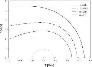
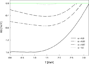
Figure 7: Left panel. Temperature dependence of pairing gap for density asymmetries $\alpha=0.0$ (solid), 0.05 (dashed-dotted), 0.07 (dashed), and 0.1 (dotted). Right panel. Temperature dependence of free energy. Labeling of asymmetries is as in the left panel.

Minimizing the free energy of an asymmetric superconductor at fixed density and temperature leads to stable solutions over the entire region of density asymmetries where non-trivial solutions of the gap equation exist.[68, 69] This can be seen in Fig. 7, where the temperature and asymmetry dependence of the pairing gap and the free-energy of a homogeneous asymmetric superconductor are shown. In particular, we see that for a fixed temperature, the gap and the free energy are single-valued functions of the density asymmetry $\alpha$ in the particle-number-conserving scheme – in contrast to what is found in the non-conserving scheme, where double-valued solutions appear.

At large asymmetries, the dependence of the gap on the temperature shows a “re-entrance” phenomenon. As the temperature is increased from low values at which the asymmetry is too large to sustain a gap, a critical temperature is reached at which pairing correlations take hold. (For example, this is seen for the $\alpha=0.1$ case in Fig. 7). This behavior can be attributed to the increase of phase-space overlap between the quasiparticles that pair, due to the thermal smearing of the Fermi surfaces. Further increase of temperature suppresses the pairing gap at a higher critical temperature due to thermal excitation of the system, in much the same way as in the symmetric superconductors. Clearly, in this scenario the pairing gap has a maximum at some intermediate temperature. The values of the two critical temperatures are controlled by different mechanisms. The superconductivity (or superfluidity) is destroyed with decreasing temperature at the lower critical temperature when the smearing of the Fermi surfaces becomes insufficient to maintain the required phase-space coherence. The upper critical temperature is the analog of the BCS critical temperature and corresponds to a transition to (re-entrance of) the normal state because of thermal excitation.

Another aspect of the asymmetric superconducting state is the gapless nature of the excitations.[70, 71] One may draw an analogy to the non-ideal Bose gas, for which only a fraction of the particles are in the zero-momentum ground state at temperatures below the critical value for Bose condensation. The dynamical properties of gapless superconductors, such as response to electroweak probes and transport, depend on the ratio $\zeta=\Delta/\delta\mu$ in an essential way: for $\zeta>1$, the response of the system is similar to that of an ordinary superconductor; in the opposite limit $\zeta<1$, the system’s behavior is essentially non-superconducting (see e.g. Ref. JAIKUMAR). These features are easily understood by examining the excitation spectrum in both limits.

1 Phases with broken space symmetries

We now turn to a special class of ASC characterized by broken global symmetries – translational, rotational, or both. In 1964, Larkin and Ovchinnikov[73] and, independently, Fulde and Ferrell[74] (LOFF) discovered that the superconducting state can sustain asymmetries beyond the Chandrasekhar-Clogston limit if electrons pair with nonzero center-of-mass (hereafter CM) momentum. The weak-coupling result for the critical shift in the Fermi surfaces for onset of the LOFF phase is $\delta\mu_{2}=0.755\,\Delta(0)\,[>\delta\mu_{1}=0.707\,\Delta(0)]$. Since the condensate wave function depends on the CM momentum of the pair, its Fourier transform will vary in configuration space, giving rise to a lattice structure. The Fulde-Ferrell state is predicated on a plane-wave form $\Delta(\bm{r})=\Delta\,{\rm exp}(-i\bm{P}\cdot\bm{r})$ for the gap function. Larkin and Ovchinnikov considered a number of lattice types and concluded that the body-centered-cubic (bbc) lattice is the most stable configuration near the critical temperature. Recent studies of this problem in the vicinity of the critical temperature employing Ginzburg-Landau theory show that the face-centered-cubic (fcc) structure is favored.[75]

For illustrative purposes, let us consider the Fulde-Ferrell state, in which case the quasiparticle spectrum is given by

$$\omega_{\pm}(\bm{P},\bm{q})=\frac{1}{2m}\left(\frac{\bm{P}}{2}\pm\bm{q}\right)^{2}-\mu_{\pm}\,,$$ (48)

where the upper sign corresponds to neutrons and the lower sign to protons. The spectrum (48) is obtained by applying the following transformation to Eq. (13): $E_{S}\to E_{S}+(P^{2}+p^{2})/2m$ and $E_{A}\to\delta\mu\pm\bm{p}\cdot\bm{P}$. Onset of the LOFF phase entails a positive increase in the quasiparticle kinetic energy $\propto Q^{2}$, which disfavors the Fulde-Ferrell state relative to the BCS state. However, the anisotropic term $\propto\bm{P}\cdot\bm{p}$, which can be interpreted as a dipole deformation of the isotropic spectrum, modifies the phase-space overlap of the fermions and promotes pairing. The LOFF phase becomes stable when the increase in the kinetic energy required to move the condensate is smaller than the reduction in potential energy made possible by the increase in the phase-space overlap. The magnitude of the total momentum serves as a variational parameter for minimization of the ground-state energy of the system.

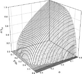
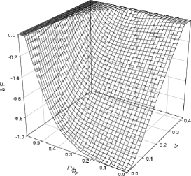
Figure 8: Left panel. Dependence of pairing gap $\Delta$ in the LOFF phase on density asymmetry $\alpha$ and total momentum $P$ of the condensate, relative to pairing gap $\Delta_{00}$ in the limit $P=0=\alpha$. Right panel. Dependence of free energy of the LOFF phase on the same quantities as in the left panel.

The pairing gap and the free energy of ASC with finite momentum are shown in Fig. 8. It is assumed that the gap function depends parametrically on the magnitude of the CM momentum, but is independent of its direction.[76] For such an Ansatz the anisotropy of the spectrum appears only in the Fermi functions in the kernels of Eqs. (18) and (19) and is averaged through the phase-space integration. It is seen in Fig. 8 that an ASC-LOFF state arises for arbitrary finite momentum of the condensate below some critical value. For large enough asymmetries the minimum of the free energy moves from $P=0$ to intermediate values of $P$, i.e., the ground state of the system corresponds to a condensate with nonzero CM momentum of Cooper pairs. Note that for the near-critical range of asymmetries, the condensate exists only in the LOFF state and its dependence on the total momentum exhibits the re-entrance behavior found in the temperature dependence of the homogeneous ASC. The order of the phase transition from the LOFF to the normal state is a complex issue that depends on the preferred lattice structure, among other things (see Ref. Casalbuoni:2003jn and work cited therein).

Due to the Pauli exclusion principle, a noninteracting fermionic gas fills an isotropic Fermi sphere; similarly, if there are two types of noninteracting fermions, each species fills an isotropic Fermi sphere. Consider now a strongly interacting system that is a Fermi liquid rather than a Fermi gas. According to Fermi-liquid theory, the states of the interacting system are reached by switching the interaction on adiabatically. Driven by this process, the noninteracting gas evolves into a strongly-interacting liquid, in which the dressed single-particle degrees of freedom – the quasiparticles – once again fill a spherical shell isotropically. However, this simple Fermi-liquid picture may not hold in two-component (or multi-component) fermionic systems in which the fermions of differing species interact via strong pairing forces. Indeed, there can exist a stable superconducting phase that sustains ellipsoidal deformations of the Fermi-surfaces, a phase hereafter referred to as deformed Fermi-surface superconductivity[78, 79] (DFS).

The quadrupole deformations of the Fermi surfaces are described by expanding the quasiparticle spectrum in spherical harmonics and keeping the $l=2$ contributions,[78, 79]

$$\omega^{D}_{\pm}(\bm{q})=\omega_{\pm}(\vec{q})+\epsilon_{2,\pm}P_{2}(x)\,,$$ (49)

where $\omega_{\pm}(\vec{q})$ is the spectrum of the homogeneous ASC and the coefficients $\epsilon_{2}$ describe the deformations of the Fermi surfaces that break the rotational O(3) symmetry down to O(2). The O(2) symmetry axis is chosen spontaneously. Thus, the quasiparticle spectrum of the DFS phase is obtained from the spectrum of homogeneous ASC by the transformations

$$E_{S}\to E_{S}+(\epsilon_{2,+}+\epsilon_{2,-})/2\mu\,,\quad E_{A}\to E_{A}+(\epsilon_{2,+}-\epsilon_{2,-})/2\mu\,.$$ (50)

We observe that the leading harmonic term responsible for deformation of either Fermi surface is that for $l=2$, not $l=1$, since the latter corresponds to a translation of one Fermi sphere relative to the other, without deformation. The deformations are deemed to be stable if they lower the free energy of the system relative to its value in the undeformed state.

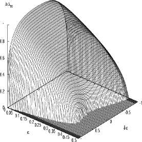
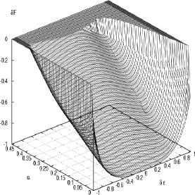
Figure 9: Left panel. Dependence of pairing gap in the DFS phase on density asymmetry and total momentum of the condensate. Right panel. Dependences of free energy of the DFS phase for the same input parameters as in Fig. 5. 

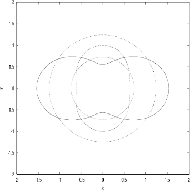
Figure 10: Projection of the Fermi surfaces on a plane parallel to the axis of symmetry breaking. The concentric circles correspond to the two populations of spin(isospin)-up and spin(isospin)-down fermions in a spherically symmetric state ($\delta\epsilon=0$), while the deformed symbols correspond to the state with relative deformation $\delta\epsilon=0.64$. The spin(isospin)-density asymmetry is $\alpha=0.35$.

The deformation parameters $\epsilon_{2\pm}$ are determined by minimization of the free energy of the system, as was done for the Cooper-pair momentum parameter $P$ in the case of broken translational invariance (LOFF states). Three-dimensional plots of the dependence of the pairing gap and free energy of the DFS phase on asymmetry and the relative deformation $\delta\epsilon=(\epsilon_{2,+}-\epsilon_{2,-})/2\mu$ are provided in Fig. 9. Fig. 10 shows a typical deformed Fermi-surface configuration that lowers the expected ground-state energy below that of the non-deformed state. At $\alpha=0$, the critical deformation for which pairing ceases is the same for prolate and oblate deformations. At finite $\alpha$ and in the positive range of $\delta\epsilon$, the maximum value of the gap is attained for constant $\delta\epsilon$; at negative $\delta\epsilon$ the maximum increases as a function of deformation and saturates for $\delta\epsilon\simeq 1$. The re-entrance phenomenon sets in for large asymmetries as $\delta\epsilon$ is increased from zero to finite values. (N.B. The essential difference between LOFF and DFS phases is that in the latter, the translational symmetry of the superconductor remains unbroken.)

To complete our discussion of pairing states in nonrelativistic asymmetric superconductors, we briefly mention some of the alternatives to the LOFF and DFS phases. One possibility is that the system prefers a phase separation of the superconducting and normal phases in real space, such that the superconducting phase contains particles with matching chemical potentials, i.e. is symmetric, while the normal phase remains asymmetric.[80]

Equal-spin (-isospin, -flavor) pairing is another option, if the interaction between like-spin particles is attractive.[81, 82] Since the separation of the Fermi surfaces does not affect spin-1 pairing on each Fermi surface, an asymmetric superconductor may evolve into a spin-1 superconducting state (rather than a non-superconducting state) as the asymmetry is increased. Therefore spin-1 pairing becomes the limiting case for very large asymmetries. If the single-particle states defining the different Fermi surfaces are characterized by spin (as is the case in the metallic superconductors), the pairing interaction in a spin-1 state should be $P$-wave and the transition is from $S$-wave to $P$-wave pairing. If the fermions are characterized by one or more additional discrete quantum numbers (say isospin as well as spin), the transition may occur between different $S$-wave phases (e.g. from isospin-singlet to isospin-triplet in the case of nuclear matter). The possibilities become especially rich in dense quark matter.

4 Crossover from BCS pairing to Bose-Einstein condensation

A crossover from BCS superconductivity to Bose-Einstein condensation (BEC) is exhibited in fermionic systems with attractive interactions under sufficient decrease of the density and/or sufficient increase of the interaction strength. The transition from large overlapping Cooper pairs to tightly bound non-overlapping bosons can be described entirely within the ordinary BCS theory, if the effects of fluctuations are ignored (mean-field approximation). Early studies of this type of transition were carried out in the contexts of ordinary superconductors,[83] excitonic superconductivity in semiconductors,[84] and, at finite temperature, an attractive fermion gas.[85] Although the BCS and BEC limits are physically quite different, the transition between them is found to be smooth within ordinary BCS theory.

Several authors have considered the BCS-to-BEC transition in the nuclear context. In isospin-symmetric nuclear matter, neutron-proton ($np$) pairing undergoes a smooth transition leading from an assembly of $np$ Cooper pairs at higher densities to a gas of Bose-condensed deuterons as the nucleon density is reduced to extremely low values.[86, 87, 88, 89, 90] This transition may be relevant – and could then yield valuable information on $np$ correlations – in low-density nuclear systems (especially the nuclear surface), in expanding nuclear matter from heavy-ion collisions, and in supernova matter. The underlying equations of the theory are (18) and (19) with $E_{A}=0$; we shall address the effects of asymmetry at a later point.

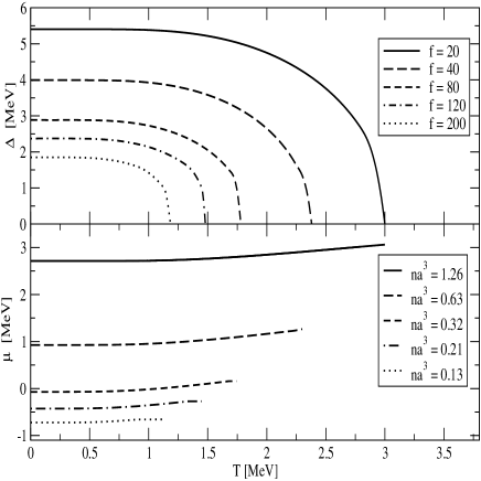
Figure 11: Dependence of pairing gap (upper panel) and chemical potential (lower panel) on temperature for fixed values of the ratio $f=n_{0}/n$, where $n$ is the baryon density and $n_{0}=0.16$ fm^-3 is the saturation density of symmetrical nuclear matter. Values of the diluteness parameter $na^{3}$ assume a scattering length $a=5.4$ fm.

The top panel of Fig. 11 shows the dependence of the gap function on temperature for several densities $n$, given in terms of the ratio $f=n_{0}/n$, where $n_{0}=0.16$ fm^-3 is the saturation density of symmetrical nuclear matter. The bottom panel shows the associated chemical potentials $\mu$ computed self-consistently from Eq. (19). The low- and high-temperature asymptotics of the gap function are well described by the BCS relations $\Delta(T\to 0)=\Delta(0)-[2\pi\alpha\Delta(0)T]^{1/2}\,{\rm exp}(-\Delta(0)/T)$ and $\Delta(T\to T_{c2})=3.06\,\beta[T_{c2}(T_{c2}-T)]^{1/2}$, respectively, where $T_{c2}$ is the critical temperature of the phase transition. However, the BCS weak-coupling values $\alpha=1=\beta$ must be replaced with $\alpha\sim 0.2$ and $\beta\sim 0.9$. As a consequence, the ratio of the zero-temperature gap to the critical temperature deviates from the familiar BCS result $\Delta(0)/T_{c2}=1.76$. Deviations from the original BCS theory are understandable in that (i) the system is in the strong-coupling regime, and (ii) the pairing is in a spin-triplet rather than a spin-singlet state. [90]

One measure of coupling strength is the ratio $\Delta(0)/|\mu|$ of the zero-temperature energy gap to the magnitude of the chemical potential. It is seen from Fig. 11 that the strong-coupling regime is realized for $f\geq 40$ (i.e., $\Delta\gg\mu$). At $f=20$ the system is in a transitional regime ($\Delta\sim\mu$). Another measure of coupling is the diluteness parameter $n|a|^{3}$, where $a$ is the scattering length. In agreement with the first criterion, the matter is in the dilute (or strong-coupling) regime for $f\geq 40$, since this range corresponds to $na^{3}=0.63<1$ when $a$ is taken as the triplet $n-p$ scattering length, 5.4 fm. A signature of the crossover from weak to strong coupling is the change of sign of the chemical potential, which occurs for $f\approx 80$ (Fig. 11), slightly below the crossover density between weak-coupling and strong-coupling regimes.

In the limit of vanishing density, $f\to\infty$, the value of the chemical potential at $T=0$ tends to $\mu(\infty)=-1.1$ MeV, which is half the binding energy of the deuteron in free space. Indeed, in this limit the gap equation reduces to the Schrödinger equation for a two-body bound state, with the chemical potential assuming the role of the energy eigenvalue.[83] Thus, the BCS condensate of Cooper pairs in the ${}^{3}S_{1}$–${}^{3}D_{1}$ state evolves into a Bose-Einstein condensate of deuterons as the system crosses over from the weak- to the strong-coupling regime. The crossover is smooth, taking place without change of symmetry of the many-body wave function.

How does isospin asymmetry affect the transition? As the system is diluted, the critical asymmetry at which the pairing disappears increases from small values of the order of 0.1 up to the asymptotic value $\alpha=1$. The reason for this behavior is that in the low-density matter, the excess neutrons do not appreciably change the wave functions of protons, which are bound into pairs.[89] At asymptotically small densities, the chemical potential of protons tends to $\mu_{p}(\infty)=-2.2$ MeV, which is just the binding energy of the system per half the number of particles bound into deuterons. The chemical potential of neutrons is determined by the excess particles in the continuum and goes asymptotically as $\mu_{n}(\infty)\to 0$ (i.e. there is ultimately no energy cost in adding a neutron to the system). Note that the asymptotic behavior described is independent of the degree of isospin asymmetry.

In closing this section, we call attention to the remarkable progress achieved during the last few years in trapping and manipulating ultracold fermion gases. The strength of the two-body interaction between the constituent fermionic atoms can be tuned using the Feshbach resonance mechanism, by varying the external magnetic field[91, 92, 93]; thus, the entire range from weak to strong couplings can be probed. Recent experiments on ultracold atomic gases have begun to explore their properties in cases where pairing occurs between atoms in different hyperfine states, which are unequally populated.[94, 95] Systems of this kind are also subject to intensive theoretical study, with specific attention to homogeneous ASC phases,[96] phases with broken symmetries[97] and their realization in finite trap geometries [98]. The universal features of ASC revealed by this effort should contribute significantly to our understanding of nucleonic pairing under isospin-asymmetric conditions.

5 Vortex states in compact stars

1 Currents and quantized circulation

The macroscopic physics of neutron-star rotation and its anomalies observed in the timing of pulsars can be described within the hydrodynamic theory of superfluids suitably extended to multifluid systems [99, 100, 101, 102, 103, 104, 105]. The elementary constituents of a Fermi superfluid – the Cooper pairs – are characterized by a coherence length $\xi$. On length scales $L\gg\xi$, the condensate of Cooper pairs can be described by a single wave function $\psi$, and the condensate forms a macroscopically coherent state. At an intermediate or “mesoscopic” scale, stellar rotation and the presence of a magnetic field lead to the formation of vortices, macroscopic quantum objects whose distinctive property is the quantization of circulation around a path encircling the vortex core. Since the condensate wave function must be single-valued at each point of the condensate, the circulation is quantized in units of $2\pi\hbar$. On writing $\psi=\psi_{0}e^{i\chi}$, the gauge-invariant superfluid velocities can be expressed through the gradient of the phase of the superfluid order parameter $\chi$ and the value of the vector potential ${\bm{A}}$:

$${\bm{v}}_{\tau}=\frac{\hbar}{2m_{\tau}}{\bm{\nabla}}\chi_{\tau}-\frac{e_{\tau}}{m_{\tau}c}{\bm{A}}\,.$$ (51)

In this expression, $e_{\tau}\equiv(e,0)$ specifies the electric charge of protons ($p$) and neutrons ($n$) respectively, $m_{\tau}$ is their bare mass, and $\tau$ stands for $n$ or $p$. Applying the curl operator to Eq. (51) and implementing quantization of the circulation (with the phase of the superfluid order parameter changing by $2\pi$ around a closed path), one finds

$$\mathop{\rm curl}{\bm{v}_{\tau}}=\frac{\pi\hbar}{m_{\tau}}{\bm{\nu}}_{\tau}\sum_{j}\delta^{(2)}({{\bm{x}}}-{{\bm{x}}}_{\tau j})-\frac{e_{\tau}}{m_{\tau}c}{\bm{B}}\equiv{\bm{\omega}}_{\tau}\,,$$ (52)

where $\pi\hbar/m_{\tau}$ is the quantum of circulation, ${\bm{\nu}}_{\tau}\equiv{\bm{\omega}}_{\tau}/\omega_{\tau}$ is a unit vector along a given vortex line, ${{\bm{x}}}_{\tau j}$ defines the position of a vortex line in the plane orthogonal to the vector ${\bm{\nu}}_{\tau}$, $\delta^{(2)}$ is a two-dimensional Dirac delta function in this plane, and ${\bm{B}}=\mathop{\rm curl}\,{\bm{A}}$ is the magnetic-field induction. The index $j$ is summed over the sites of vortex lines. Eq. (52) treats the vortex cores as singularities in the plane orthogonal to $\bm{\nu}_{\tau}$; this simplification is justified on scales larger than the coherence length of the condensate. For a single vortex, the integral of Eq. (52) completely determines the superfluid pattern. Since this equation is linear, the superfluid pattern created by a larger number of vortices is formed by superposition of the flows induced by each vortex. Obviously, the resulting net flow depends on the arrangement of the vortices.

The condensate wave function can be written as $\psi({\bm{x}})=f(r)e^{i\theta}$ in cylindrical polar coordinates $(r,\theta,z)$. Upon integrating Eq. (52), the neutron and proton superfluid velocities then become

$${\bm{v}}_{n}(r)=\frac{\hbar}{2m_{n}r}\hat{\theta}\,,\quad\quad{\bm{v}}_{p}(r)=\frac{\hbar}{2m_{p}\lambda}K_{1}\left(\frac{r}{\lambda}\right)\hat{\theta}\,,$$ (53)

where $K_{1}$ is the Bessel function of imaginary argument. The divergence of the neutron-vortex velocity ${\bm{v}}_{n}(r)$ as $r\to 0$ is regularized by a cutoff $\Lambda\sim\xi_{n}$. The long-range nature of ${\bm{v}}_{n}(r)$ results in slow falloff of a density perturbation in the condensate. In a proton vortex, the supercurrent is screened exponentially on length scales of the order of the penetration depth $\lambda$. Thus, for $r\gg\lambda$, $K_{1}(r/\lambda)\simeq{\rm exp}(-r/\lambda)$.

On global, hydrodynamic scales, transition to a continuum vortex distribution can be carried through on the right-hand side of Eq. (52) by defining vortex densities $n_{\tau}=\sum_{j}\delta^{(2)}({\bm{x}}-{\bm{x}}_{\tau j})$. Since the curl of ${\bm{v}}_{n}$ is simply $2\Omega$ for rigid-body rotations, the number density of vortices in the neutron superfluid is related to the macroscopic angular velocity of the neutron condensate by the Feynman formula

$$n_{n}=\frac{2m_{n}\Omega}{\pi\hbar}\,.$$ (54)

For typical pulsar periods $P$ in the range $0.05<P<0.5$ s, one has $n_{n}\simeq 6.3.\times 10^{3}~{}P^{-1}\sim 10^{4}$–$10^{5}$ per cm². In the case of a charged superfluid, Eq. (52) can be transformed to a contour integral over a path along which ${\bm{v}}_{p}=0$, since the supercurrent is screened beyond the magnetic field penetration depth $\lambda$. If the proton superfluid is a type-II superconductor (i.e., $\lambda/\xi_{p}>1/\sqrt{2}$), the continuum vortex limit leads to the estimate

$$n_{p}=\frac{B}{\Phi_{0}}\simeq 5\times 10^{18}~{}{\rm cm}^{-2}\,,$$ (55)

where $\Phi_{0}=\pi\hbar c/e$ is the flux quantum. We note that the number of proton vortices per neutron vortex is $n_{p}/n_{n}\sim 10^{13}-10^{14}$, independently of their arrangement. The energy of a bundle of neutron or proton vortices is minimized by a triangular lattice with a unit cell area $n_{\tau}^{-1}=(\sqrt{3}/2)\,d_{\tau}^{2}$. The lengths of “basis vectors” of the lattices in the neutron and proton condensates (the inter-vortex distances) are

$$d_{n}=\left(\frac{\pi\hbar}{\sqrt{3}\,m_{n}\,\Omega}\right)^{1/2}\,,\quad\quad d_{p}=\left(\frac{2\,\Phi_{0}}{\sqrt{3}\,B}\right)^{1/2}\,,$$ (56)

where $B$ is the mean magnetic-field induction. Using the estimates given in Eqs. (54) and (55), one finds that the neutron and proton inter-vortex distances are $d_{n}\sim 10^{-2}-10^{-3}$ cm and $d_{p}\sim 10^{-9}$ cm, respectively. For typical values of the microscopic parameters, the penetration depth is of the order $100~{}{\rm fm}=10^{-11}$ cm. Therefore the conditions $\xi_{n}\ll d_{n}$ and $\xi_{p}\ll{\rm min}(\lambda,\,d_{p})$ are satisfied, and the use of hydrodynamics on the local scale is valid. It is also clear that global hydrodynamics can be applied on scales that are much larger than $d_{n}$ (a fraction of millimeter).

The strong interaction between the neutron and proton fluids gives rise to the entrainment effect: the supercurrent is a linear combination of the velocities of both fluids.[99, 106] More specifically, the mass current and velocity vectors are related by a nondiagonal density matrix in isospin space,

$$\left(\begin{array}[]{c}{\bm{p}}_{1}\\ {\bm{p}}_{2}\end{array}\right)=\left(\begin{array}[]{cc}\rho_{11}&\rho_{12}\\ \rho_{21}&\rho_{22}\end{array}\right)\left(\begin{array}[]{c}{\bm{v}}_{1}\\ {\bm{v}}_{2}\end{array}\right)\,,$$ (57)

where 1 and 2 label the isospin projections. The off-diagonal elements, which would vanish in the noninteracting limit, are evidently responsible for the entrainment effect. One fundamental consequence of this effect is that the neutron vortex carries a non-quantized magnetic flux[99, 106] of the same order of magnitude as the flux quantum $\Phi_{0}$. If the proton fluid forms a type-II superconductor, the number of proton vortices (sometimes called flux tubes) is $10^{12}-10^{13}$ per neutron vortex [see Eq. (55)]. Accordingly, the neutron-vortex motion (dynamics) is likely to be affected by the proton-vortex array.

The arrangement of the proton-vortex lattice is a complex issue, and there exist several models for its configuration.

• A class of (flux-tube) models envisions the proton-vortex array to be spatially homogeneous, the vorticity vector being inclined by some angle with respect to the spin vector.[107] Further, it is assumed that the flux tubes act as extended pinning centers for neutron vortices. In such models, a change in the neutron-vortex distribution is achieved by vortex creep of neutron vortices through the array of flux tubes.

• Vortex cluster models predict clustering of proton vortices over about $10\%$ of the area occupied by a neutron vortex. One particular model generates a bundle of proton vortices coaxial with the neutron vortex, through the entrainment currents induced by neutron-vortex circulation.[108] This gives rise to an average axisymmetrical magnetic field whose magnitude is compatible with pulsar observations.

• The homogeneous distribution of proton vortices could be generically unstable towards phase separation between a phase containing dense mesh of proton vortices and a phase devoid of vortices. A necessary condition is that the vortex lattice is sufficiently dilute, the mean intervortex distance being much larger than the penetration depth.[109]

• Proto-neutron stars are likely to possess natal magnetic fields; the nucleation of such a field will be associated with a first-order normal-superconducting phase transition, squeezing the field into bubbles of superconducting regions with high $B\sim 10^{14}$ G, and forming stable protonic vortex arrays which again cover about $10\%$ of the total area.[110] The dynamics of the neutron-vortex array in vortex-cluster models is controlled by the electromagnetic scattering of electrons off a vortex cluster.

Current models of BCS pairing of protons do not exclude the possibility that there is a transition from type-II to type-I superconductivity of protons as the density is increased.[111] Type-I superconducting protons will have domain structures analogous to those observed in laboratory experiments on terrestrial superconducting materials. The electrodynamics of the proton domain structures in NS can be treated by adapting the theories developed for laboratory superconductors, in which the magnetic fields are generated by normal currents driven around a cylindrical cavity by temperature gradients.[112] A recent theoretical study[113] examined the effect of interactions between neutron and proton Cooper pairs on the status of proton superconductivity. The results suggest that type-I superconductivity can be enforced throughout the entire stellar core if the strength of the interaction between Cooper pairs is significant. However, within the mean-field BCS theory, the Cooper pairs are noninteracting entities, and any deviations from this picture must be due to fluctuations. Alford et al.[114] estimated the strength of the interaction between neutron and proton Cooper pairs due to fluctuations and found it to be too small to account for the interactions assumed in Ref. BUCKLEY. Nevertheless, type-I superconductivity of protons is not excluded by current calculations of ${}^{1}S_{0}$ pairing of protons, and we shall address below its potential implications for the macroscopic manifestations of superfluidity in neutron stars.

2 Constraints placed by neutron-star precession on the mutual friction between superfluid and normal-fluid components

Since most of the inertia of a NS is carried by the neutron superfluids in the core and in the crust, the key to an understanding of NS rotational anomalies lies in the transfer of angular momentum from the superfluid to the normal (unpaired) component of the star, whose rotation is observed through the magnetospheric emission. At the local hydrodynamical scale, the rate of angular momentum transfer between the superfluid and normal components is determined by the equation of motion of a superfluid neutron vortex line. In the approximation that the inertial mass of the vortex is neglected, the equation of motion is

$$\omega_{S}(\bm{v}_{S}-\bm{v}_{L})\times\bm{\nu}+\zeta(\bm{v}_{L}-\bm{v}_{N})+\zeta^{\prime}(\bm{v}_{L}-\bm{v}_{N})\times\bm{\nu}=0\,,$$ (58)

where $\bm{v}_{S}$ and $\bm{v}_{N}$ are the superfluid and normal fluid velocities, $\bm{v}_{L}$ is the velocity of the vortex, $\bm{\nu}$ is a unit vector along the vortex line, $\omega_{S}$ is the unit of circulation, and $\zeta$, $\zeta^{\prime}$ are (dimensionless) friction coefficients, also known as the drag-to-lift ratios. These coefficients encode the essential information on the microscopic processes of interaction of vortices with the ambient unpaired fluid. Microscopic calculations commonly indicate $\zeta^{\prime}\approx 0$, and one is left with a single parameter $\zeta$.

In the NS crust, neutron vortices are embedded in a lattice of neutron-rich nuclei, and the $\zeta$ coefficient is determined by the interaction of the vortices with the nuclei and the electron plasma. (In some models, neutron vortices are localized – pinned to the nuclei or situated in between them.[115, 116] If the pinning is strong, Eq. (58) is not valid, since the forces acting on the vortex are not linear functions of velocities. However, the regime of perfect pinning can be identified with the $\zeta\to\infty$ limit.) In the core of the star, the friction is controlled by the interaction of neutron vortices with the ambient electron-proton plasma; Eq. (58) is valid under these conditions. Initial studies of the dynamical coupling between the superfluid and the normal fluid focused on interpretation of the observed post-glitch relaxation of pulsar rotational periods. It turns out that such interpretation is fraught with ambiguity, because the long relaxation times can be obtained in the two opposite limits of weak ($\zeta\to 0$) and strong ($\zeta\to\infty$) couplings.

Recent observation[3] of long-term periodic variabilities in PSR B1828-11, if attributed to precession of this pulsar, challenges existing theories of vortex dynamics in NS.[117, 118, 119] The importance of the inferred precession mode stems from the fact that it involves non-axisymmetric perturbations of the rotational state, removing the degeneracy with respect to $\zeta$ that is inherent in the interpretation of post-glitch dynamics. In the frictionless limit, a star must precess at the classical frequency $\epsilon\Omega$, where $\epsilon$ is the eccentricity and $\Omega$ is the rotation frequency. Clearly, then, there must exist a crossover from damped to free precession as $\zeta$ is decreased. The crossover is determined by the dimensionless parameters ($I_{S}/I_{N})\beta$ and ($I_{S}/I_{N})\beta^{\prime}$. Here, $\beta=\zeta/[(1-\zeta^{\prime})^{2}+\zeta^{2}]$, $\beta^{\prime}=1-\beta(1-\zeta^{\prime})/\zeta$, $I_{S}$ is the moment of inertia of the superfluid, and $I_{N}$ is the moment of inertia of the crust plus any component coupled to it on time scales much shorter than the precession time scale. The precession frequency is[118]

$$\Omega_{P}=\epsilon\Omega_{S}\left[\left(1+\beta^{\prime}\frac{I_{S}}{I_{N}}\right)+i\beta\frac{I_{S}}{I_{N}}\right]\,,$$ (59)

where $\Omega_{S}$ is the spin frequency and $\epsilon$ is the eccentricity. A no-go theorem[118] states that Eulerian precession in a superfluid neutron star is impossible if ($I_{S}/I_{N})\zeta>1$ (assuming as before $\zeta^{\prime}\to 0$). There is a subtlety in this result: the precession is impossible because the precession mode, apart from being damped, is renormalized by the non-dissipative component of the superfluid/normal-fluid interaction ($\propto\beta^{\prime})$. In effect, the value of the precession eigenfrequency drops below the damping frequency for any $\zeta$ larger than the crossover value. This counterintuitive result cannot be obtained from arguments based solely on dissipation. In fact, according to Eq. (59), the damping time scale for precession increases linearly with $\zeta$, and in the limit $\zeta\to\infty$ one would (wrongly) predict undamped precession. If a neutron star contains multiple layers of superfluids, the picture is more complex, but the generic features of the crossover are the same.[118] While it is common to study perturbations from the state of uniform rotation, the precessional state may actually correspond to the local energy minimum of an inclined rotor if there is a large enough magnetic stress on the star’s core.[120, 121]

In the core of a neutron star, the quantized neutron-vortex array is embedded in an electron-proton plasma, with the protons in a superconducting state. Electrons will scatter off the anomalous magnetic moments of (ungapped) neutron quasiparticles localized in the core of a neutron vortex.[122] Because of the ${}^{3}P_{2}$ spin-1 nature of the order parameter of the neutron superfluid in the core, the ${}^{3}P_{2}$ vortex core has an additional magnetization that scatters electrons more effectively.[123] An even more efficient scattering mechanism comes into play due to the flux $\sim\Phi_{0}$ induced by the proton supercurrent on the neutron vortex via the entrainment effect.[106] If the protons are non-superconducting in some regions of the core, then the strong nuclear interaction between protons and neutron quasiparticles localized within a vortex core leads to an efficient coupling of the electron-proton plasma and the neutron superfluid.[124] The above models belong to the class of weak-coupling theories, i.e. $\zeta\ll 1$, and, according to the no-go theorems, are compatible with free precession of the neutron star. However, these theories of mutual friction assume (unrealistically) that the proton-vortex lattice has no effect whatsoever on neutron-vortex dynamics in the core.

The mechanism underlying mutual friction in the flux-tube models is the slow motion of neutron vortices through the pinning barriers (here, flux tubes) via thermally activated creep. Since, in general, the creep models presume that the vortex lattice closely follows the rotation of the pinning centers (N.B. the case of perfect pinning corresponds to $\zeta\to\infty$), the effective friction in these models is large,[125] $\zeta\gg 1$. The kelvon-vortex coupling in the core provides another interaction channel, leading again to[119] $\zeta\gg 1$. Similarly, for vortex-cluster models, in which the neutron-vortex lattice and the associated proton-vortex cluster move coherently, electron scattering by proton-vortex clusters also gives[102] $\zeta\gg 1$. Accordingly, these theories are incompatible with free precession of a neutron star. This conclusion has been stressed by Link,[119] and it has been argued that type-I superconductivity could be an alternative.

In the crust of a neutron star, the neutron-vortex lattice is embedded in a lattice of nuclei and the charge-neutralizing background created by an almost homogeneous electron sea. In the vortex-creep models, the neutron-vortex lattice maintains rotational equilibrium via thermal and quantal creep through the pinning barriers (nuclei).[115, 116] Hence these models imply $\zeta\gg 1$ and are incompatible with free precession. If the pinning is absent, either because re-pinning cannot be achieved in post-jump equilibrium [126] and/or because of mutual cancellation of the forces from different pinning centers, the freely flowing neutron-vortex lattice interacts with the electron-phonon component of the crust. These interactions are weak and lead to[127, 128] $\zeta\ll 1$. Note that the above estimates assume that the ratio $I_{S}/I_{N}$ is roughly of order unity. While it is difficult to estimate this ratio precisely, it is unlikely to differ from unity by many orders of magnitude.

3 Type-I superconductivity in neutron stars

The equilibrium structure of alternating superconducting and normal domains in a type-I superconductor is a complicated problem that depends on, among other things, the nucleation history of the superfluid phase. By flux conservation, the ratio of the sizes of the superfluid and normal domains is given by the relation $d_{S}/d_{N}=\sqrt{H_{\rm cm}/B}\sim 10$, where $B\sim 10^{12}$ G is the average value of the magnetic induction and $H_{\rm cm}\sim 10^{14}$ G is the thermodynamic critical magnetic field.

We first examine a model[111] in which the magnetic field generated by the entrainment effect supports the formation of domains coaxial with the neutron vortex. Consider a vortex that moves at a constant velocity $\bm{v}_{L}$ and carries a coaxial normal domain of protonic fluid relative to the background electron liquid. Continuity of the electrochemical potentials of the superfluid and normal phases across the boundary between them entails the existence of a constant transverse electric field

$$E=-\frac{m_{p}^{*}v_{L}v_{p}(a)}{ea}$$ (60)

across the normal domain (see Fig. 12).

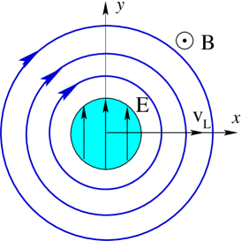
Figure 12: The structure of a rotational vortex placed in a type-I superconductor. The vortex velocity field is indicated by the concentric circles. The non-superconducting domain (shaded region) of radius $a$ is coaxial with the vortex and carries a magnetic field $H_{\rm cm}\sim 10^{14}$ G. The vortex motion along the $x$-axis generates a transverse electric field, which drives the electron current through the domain and causes Ohmic dissipation.

The energy dissipated per unit length of a vortex is $W=\sigma E^{2}\,(a/b)^{2}$, where $\sigma$ is the electrical conductivity and the factor $(a/b)^{2}$ is the fractional area occupied by the domain. Combining this relation with Eq. (60), we obtain an alternative expression $W=\eta v_{L}^{2}$ for the dissipation, which identifies the friction coefficient as[129]

$$\zeta=\frac{\eta}{\rho_{S}\omega_{S}}=\frac{\sigma}{\rho_{S}\omega_{S}c^{2}}\left(\frac{\Phi_{1}}{2\pi ab}\right)^{2}\left[\frac{a}{\lambda}{\rm ln}\left(\frac{b}{a}\right){\rm coth}\left(\frac{b-a}{a}\right)-1\right]^{2}\,,$$ (61)

where $\Phi_{1}=(\rho_{12}/\rho_{11})\Phi_{0}$. The zero-field conductivity of ultra-relativistic electrons is $\sigma_{0}=n_{e}e^{2}c\tau_{c}/p_{eF}$, where $p_{eF}$ is the electron Fermi momentum, $n_{e}$ is the electron number density, and $\tau_{c}$ is the relaxation time for Coulomb scattering of electrons off protons in the normal domains.[14] The conductivity $\sigma={\sigma_{0}}/{(\omega_{c}\tau_{c})^{2}}$ entering Eq. (61) includes the effect of the bending of electron trajectories in the magnetic field. In this formula, $\omega_{c}=eH_{cm}/p_{F}$ is the electron cyclotron frequency, which is proportional to the thermodynamic critical field $H_{cm}$. For the typical density range $\rho=(7.9-8.6)\times 10^{14}$ g/cm³, the friction coefficient has the order of magnitude $\zeta\simeq 10^{-5}$ at the temperature $T=10^{8}$ K and scales with temperature as $\zeta\propto T^{2}$. The drag-to-lift ratio satisfies the condition $\zeta\ll 1$ for all $T$ below the critical temperature of the superfluid phase transition.

We turn next to the friction coefficient as predicted by the model of Buckley et al.,[113] in which the normal domains contain a large number $N\sim 10$ neutron vortices. In this case, the damping of the differential rotation between the electron-proton plasma and the neutron superfluid is due to the interaction of domain (i.e., non-superconducting) protons with the core quasiparticles confined in the neutron-vortex core. The relaxation process is therefore the same as in the case where the proton fluid is non-superconducting over the entire bulk of the core. However, the result needs to be rescaled by the ratio of the areas occupied by the normal and superconducting layers. The relaxation time per single vortex is[124]

$$\tau_{np}=6\left(\frac{p_{Fp}}{p_{Fn}}\right)^{4}\frac{m_{n}\mu_{pn}^{*}}{\hbar m_{p}^{*}T\sigma_{np}}\,{\rm exp}\left(0.02\frac{\Delta_{n}^{2}}{\epsilon_{Fn}T}\right)\,,$$ (62)

where $p_{Fp}$ and $p_{Fn}$ are the Fermi momenta of protons and neutrons, $\mu_{pn}^{*}=m_{p}^{*}m_{n}^{*}/(m_{p}^{*}+m_{n}^{*})$ is the reduced effective mass in terms of the proton and neutron effective masses, $\sigma_{np}$ is the total in-medium neutron-proton scattering cross section, $\Delta_{n}$ is the gap in the neutron quasiparticle spectrum, and $\epsilon_{Fn}$ is the neutron Fermi energy. [Eq. (62) differs from the analogous expression in Ref. SEDRAKIAN98 by the factor $4m_{n}/\hbar P$; here $P$ is the pulsar period and $m_{n}$ is the free-space neutron mass.]

In the relaxation-time approximation and zero-temperature limit, the friction is written as

$$\zeta=\frac{\eta}{\rho_{S}\omega_{S}}=\frac{\hbar p_{Fp}n_{p}}{\rho_{S}\omega_{S}c\tau_{np}}\,,$$ (63)

where $n_{p}$ is the proton number density. For proton densities in the range $\rho_{p}=(4-8)\times 10^{14}$ g/cm³ and temperatures $T\sim 10^{7-8}$, one finds $\zeta\leq 0.1$. For a given model of the type-I superconducting structure, the friction coefficient $\zeta$ must be rescaled by a factor $(d_{N}/d_{S})^{2}\sim 0.01$.

Now we are in a position to discuss the implications of the friction mechanisms described above for neutron-star precession. The condition $(I_{S}/I_{N})\zeta<1$ seems to fulfilled unless $I_{S}/I_{N}\gg 1$. The magnitude of the ratio $I_{S}/I_{N}$ depends on the superfluid/normal-fluid friction within all superfluid regions of the neutron star and is hard to assess. Glitches and post-glitch relaxation provide a model-independent lower bound, $I_{S}/I_{N}\geq 0.1$. On the other hand, an upper bound is difficult to set. The deep interior of the star, if superfluid, could be decoupled from the observable parts of the star on evolutionary time scales, without any effect on short-time-scale physics (although one does require $\zeta\to 0$, rather than $\zeta\to\infty$, to prevent damping of the precession). At any rate, it is rather unlikely that $I_{S}/I_{N}$ exceeds unity by many orders of magnitude, and appealing to the lower bound on the ratio of the moments of inertia, one can conclude that the precession is undamped for both dissipation mechanisms considered.

6 Concluding remarks

This review has covered a number of aspects of nucleonic superfluidity, ranging from microscopic theories of pairing in nuclear systems and neutron stars to mesoscopic frictional processes in superfluids and rotational anomalies in pulsars. Our survey of this important subfield is by no means complete. While the selection of topics is naturally biased toward the primary interests of the authors, we have chosen topics and problems with the intent of elucidating (i) the fascinating relationships between the physics involved at different scales and (ii) the richness of the contributions from diverse subfields of physics. We close by listing a number of issues and problems that call for further clarification and concerted effort within the general framework of our discussions.

• The pairing problem at the level of mean-field BCS theory, with the pairing driven directly by in-vacuum nuclear interactions, is essentially solved within the density range over which these interactions are constrained by experiment. On the other hand, issues such as the screening of nuclear interactions, renormalization of the single-particle spectrum, and off-shell energy behavior of the pairing gap still defy quantitative resolution. Broadly speaking, extensions beyond the BCS theory are needed that incorporate fluctuation corrections while providing a consistent treatment of short-range correlations.

• Superfluid phases with broken space-time symmetries have received much attention from theorists in recent years, while experimental realization of asymmetric superfluids opens the possibility of testing the predictions of theory. Importantly, relevant experiments are now probing the BCS-BEC crossover via the Feshbach resonance mechanism. Given a broad effort, there is the prospect of mapping out the superfluid phase diagrams of interesting fermionic systems, both experimentally and theoretically, in the space of coupling strength, spin/isospin asymmetries, temperature, etc.

• The rotational anomalies observed in neutron stars continue to provide useful constraints on the state of the superfluid matter in neutron-star interiors. Further theoretical studies of vortex dynamics, combined with pulsar timing observations, may be expected to shed new light on the internal structure of the superfluid phases of neutron stars, especially on the question whether protons form a type-I or type-II superconductor.

Acknowledgments

We acknowledge useful interactions with A. Bulgac, J. M. Cordes, W. H. Dickhoff, J. Dukelsky, V. A. Khodel, B. Link, U. Lombardo, H. Müther, A. Polls, P. Schuck, H.-J. Schulze, I. Wasserman, D. N. Voskresensky and M. V. Zverev. AS acknowledges research support through a Grant from the SFB 382 of the Deutsche Forschungsgemeinschaft; JWC, through Grant No. PHY-0140316 from the U.S. National Science Foundation.

References

- [1] S. L. Shemar and A. G. Lyne, Mon. Not. RAS 282, 677 (1996).
- [2] J. M. Cordes, G. S. Downs, and J. Krause-Polstorff, Astrophys. J. 330, 847 (1988).
- [3] I. H. Stairs, A. G. Lyne, and S. L. Shemar, Nature 406, 484 (2000).
- [4] D. N. Voskresensky, Lecture Notes in Physics vol. 578 (Springer-Verlag, New York, 2001) pg. 467.
- [5] D. G. Yakovlev and C. J. Pethick, Ann. Rev. Astron. Astrophys. 42, 169 (2004).
- [6] D. Page, U. Geppert, and F. Weber, Nucl. Phys. A., in press.
- [7] A. Sedrakian, Prog. Part. Nucl. Phys., in press, nucl-th/0601086.
- [8] L. Lindblom and G. Mendell, Phys. Rev. D 61, 4003 (2000).
- [9] A. Sedrakian and I. Wasserman, Phys. Rev. D 63, 024016 (2000).
- [10] N. Andersson, G. L. Comer, and K. Grosart, Mon. Not. RAS 355, 918 (2004).
- [11] A. B. Migdal, Zh. Eksp. Teor. Fiz. 37, 249 (1959) [Sov. Phys. JETP 10, 176 (1960).]
- [12] A. Bohr, B. Mottelson, and D. Pines, Phys. Rev. 110, 936 (1958).
- [13] L. N. Cooper, R. L. Mills, and A. M. Sessler, Phys. Rev. 114, 1377 (1959).
- [14] G. Baym, C. J. Pethick, and D. Pines, Nature 224, 673 (1969).
- [15] C.-H. Yang and J. W. Clark, Nuovo Cimento Lett. 3, 272 (1970); ibid. 2, 379 (1970).
- [16] C.-H. Yang and J. W. Clark, Nucl. Phys. A 174, 49 (1971); C.-H. Yang Ph.D. Thesis, Washington University in St. Louis (1971).
- [17] N.-C. Chao, J. W. Clark, and C.-H. Yang, Nucl. Phys. A179, 320 (1972).
- [18] M. Hoffberg, A. E. Glassgold, R. W. Richardson, and M. Ruderman, Phys. Rev. Lett. 24, 775 (1970).
- [19] T. Takatsuka, Prog. Theor. Phys. 48, 1517 (1972).
- [20] M. Baldo, O. Elgaroey, L. Engvik, M. Hjorth-Jensen, H.-J. Schulze, Phys. Rev. C 58, (1998) 1921.
- [21] M. V. Zverev, J. W. Clark, V. A. Khodel Nucl. Phys. A 720, 20 (2003); J. W. Clark, V. A. Khodel, M. V. Zverev, nucl-th/0203046; V. A. Khodel, J. W. Clark, M. V. Zverev, Phys. Rev. Lett. 87, 031103 (2001); V. V. Khodel, V. A. Khodel, J. W. Clark, Nucl. Phys. A 679, 827 (2001); V. A. Khodel, J. W. Clark, M. Takano, and M. V. Zverev, Phys. Rev. Lett. 93, 151101 (2004).
- [22] T. Takatsuka and R. Tamagaki, Prog. Theor. Phys. Suppl. 112, 27 (1993).
- [23] A. Sedrakian, G. Röpke, and T. Alm, Nucl. Phys. 594, 355 (1995); T. Alm, G. Röpke, A. Sedrakian, and F. Weber, Nucl. Phys. A 604, 491 (1996).
- [24] T. Alm, G. Röpke, and M. Schmidt, Z. Phys. A 337, 355 (1990).
- [25] B. E. Vonderfecht, C. C. Gearhart, W. H. Dickhoff, A. Polls, and A. Ramos, Phys. Lett. B 253, 1 (1991).
- [26] M. Baldo, I. Bombaci, and U. Lombardo, Phys. Lett. B 283, 8 (1992); M. Baldo, U. Lombardo, H.-J. Schulze, and Z. Wei Phys. Rev. C 66, 054304 (2002); C. Shen, U. Lombardo, and P. Schuck Phys. Rev. C 71, 054301 (2005).
- [27] H. Müther and W. H. Dickhoff, Phys. Rev. C 72, 054313 (2005).
- [28] U. Lombardo and H.-J. Schulze, Lecture Notes in Physics, vol 578, pg 30 (Springer, Berlin).
- [29] D. J. Dean and M. Hjorth-Jensen, Rev. Mod. Phys. 75, 607 (2003).
- [30] A. A. Abrikosov, L. P. Gorkov, and I. E. Dzyaloshinski, Methods of Quantum Field Theory in Statistical Physics (Prienice-Hall, Englewood Cliffs, NJ, 1963) (Dover, New York, 1975).
- [31] A. B. Migdal, Theory of Finite Fermi-Systems (Nauka, Moscow, 1983, in Russian).
- [32] M. Baldo and A. Grasso, Phys. Lett. 485, 115 (2000).
- [33] U. Lombardo, P. Schuck, and W. Zuo, Phys. Rev C 64, 021301 (2001).
- [34] V. V. Khodel, V. A. Khodel, and J. W. Clark, Nucl. Phys. A598, 390 (1996).
- [35] A. Sedrakian, T. T. S. Kuo, H. Müther, and P. Schuck Phys. Lett. B 576, 68 (2003).
- [36] D. Pines and C. Pethick, in Proc. XIth Intern. Conf. on Low Temperature Physics, ed. E. Kandu, (Kligatu Publ. Co. Tokyo, 1971).
- [37] J. W. Clark, C. G. Källman, C. H. Yang, and D. A. Chakkalakal, Phys. Lett. B 61, 331 (1976).
- [38] S. Babu and G. Brown, Ann. Phys. 78, 1 (1973).
- [39] S.-O. Bäckman, G. E. Brown, and J. A. Niskanen, Phys. Rep. 124, 1 (1985).
- [40] W. H. Dickhoff, A. Faessler, H. Müther, and S.-S. Wu, Nucl. Phys. A 405, 534 (1983).
- [41] T. L. Ainsworth, J. Wambach, and D. Pines, Phys. Lett. B 222, 173 (1989).
- [42] J. Wambach, T. L. Ainsworth, and D. Pines, Nucl. Phys. A 555, 128 (1993).
- [43] E. Feenberg, Theory of quantum fluids (Academic Press, NY 1969).
- [44] J. W. Clark, Prog. Part. Nucl. Phys. 2, 89 (1979).
- [45] J. W. Clark and P. Westhaus, Phys. Rev. 141, 833 (1966).
- [46] J. W. Clark, L. R. Mead, E. Krotscheck, K. E. Kürten, and M. L. Ristig, Nucl. Phys. A 328, 45 (1979).
- [47] E. Krotscheck, R. A. Smith, and A. D. Jackson, Phys. Rev. B 24, 6404 (1981).
- [48] J. M. C. Chen, J. W. Clark, E. Krotscheck, and R. A. Smith, Nucl. Phys. A 451, (1986) 509.
- [49] J. M. C. Chen, J. W. Clark, R. D. Davé, and V. V. Khodel Nucl. Phys. A 555, 59 (1993).
- [50] A. Fabrocini, S. Fantoni, A. Illarionov, and K. E. Schmidt, Phys. Rev. Lett. 95, 192501 (2005).
- [51] H.-J. Schulze, J. Cugnon, A. Lejune, M. Baldo, and U. Lombardo, Phys. Lett. B 375, 1 (1996).
- [52] A. Schwenk, B. Friman, and G. Brown, Nucl. Phys. A 713, 191 (2003).
- [53] T. Ericson and W. Weise, Pions and Nuclei (Claredon Press, Oxford, 1988).
- [54] A. Sedrakian, Phys. Rev. C 68, 065805 (2003).
- [55] G. M. Eliashberg, Zh. Eksp. Teor. Fiz. 38, 966 (1960) [Sov. Phys. JETP 11, 696 (1960)].
- [56] V. A. Khodel, J. W. Clark, M. Takano, and M. V. Zverev, Phys. Rev. Lett. 93, 151101 (2004).
- [57] E. Krotscheck and J. W. Clark, Nucl. Phys. A 328, 73 (1979).
- [58] E. Krotscheck and J. W. Clark, Nucl. Phys. A 333, 77 (1980).
- [59] R. B. Wiringa, V. G. J. Stoks, and R. Schiavilla, Phys. Rev. C 51, 38 (1995).
- [60] S. Fantoni, Nucl. Phys. A 363, 381 (1981).
- [61] S. Fantoni and S. Rosati, Nuovo Cim. 25A, 593 (1975).
- [62] A. Schwenk and B. Friman, Phys. Rev. Lett. 92, 082501 (2004).
- [63] T. Takatsuka and R. Tamagaki, Prog. Theor. Phys 65, 1333 (1981).
- [64] A. M. Clogston, Phys. Rev. Lett. 9, 266 (1962).
- [65] B. S. Chandrasekhar, Appl. Phys. Lett. 1, 7 (1962).
- [66] G. Sarma, Phys. Chem. Solids 24, 1029 (1963).
- [67] L. P. Gor’kov and A. I. Rusinov, Zh. Eksp. Teor. Fiz. 46, 1363 (1964) [Sov. Phys. JETP 19, 922 (1964)].
- [68] A. Sedrakian, T. Alm, and U. Lombardo, Phys. Rev. C 55, R582 (1997).
- [69] A. Sedrakian and U. Lombardo, Phys. Rev. Lett. 84, 602 (2000).
- [70] M. Alford, J. Berges, and K. Rajagopal, Phys. Rev. Lett. 84, 598 (2000).
- [71] I. A. Shovkovy, S. B. Ruester, D. H. Rischke, J. Phys. G 31, 849 (2005) and refs. therein.
- [72] P. Jaikumar, C. D. Roberts, and A. Sedrakian, Phys. Rev. C 73, 042801 (2006).
- [73] A. I. Larkin and Yu. N. Ovcihnnikov, Zh. Eksp. Teor. Fiz. 47, 1136 (1964) [Sov. Phys. JETP 20, 762 (1965)].
- [74] P. Fulde and R. A. Ferrell, Phys. Rev. 135, A550 (1964).
- [75] J. A. Bowers and K. Rajagopal, Phys. Rev. D 66, 065002 (2002).
- [76] A. Sedrakian, Phys. Rev. C 63, 025801 (2001).
- [77] R. Casalbuoni, R. Gatto, M. Mannarelli, and G. Nardulli, Phys. Rev. D 66, 014006 (2002).
- [78] H. Müther and A. Sedrakian, Phys. Rev. Lett. 88, 252503 (2002); Phys. Rev. C 67, 015802 (2003).
- [79] A. Sedrakian, J. Mur-Petit, A. Polls, and H, Müther, Phys. Rev. A 72, 013613 (2005).
- [80] P. F. Bedaque, H. Caldas, and G. Rupak, Phys. Rev. Lett. 91, 247002 (2003); H. Caldas, Phys. Rev. A 69, 063602 (2004)
- [81] R. Combescot, Europhys. Lett 55, 15 (2001).
- [82] E. Gubankova, E.G. Mishchenko, and F. Wilczek, Phys. Rev. Lett. 94, 110402 (2005).
- [83] A. J. Leggett, in Modern Trends in the Theory of Condensed Matter (Springer, Berlin, 1980), p.13; J. Phys. (Paris) 41, (1980) C7-19.
- [84] L. V. Keldysh and Yu. V. Kopaev, Sov. Phys. Solid State 6, 2219 (1965); L. V. Keldysh and A. N. Kozlov, Sov. Phys. JETP 27, 521 (1968).
- [85] P. Nozières and S. Schmitt-Rink, J. Low Temp. Phys. 59, 195 (1985).
- [86] T. Alm, B. L. Friman, G. Röpke, and H. Schulz, Nucl. Phys. A 551, 45 (1993).
- [87] M. Baldo, U. Lombardo, and P. Schuck, Phys. Rev. C 52, 975 (1995).
- [88] H. Stein, A. Schnell, T. Alm, and G. Röpke, Z. Phys. A 351, 295 (1995).
- [89] U. Lombardo, P Nozières, P. Schuck, H.-J. Schulze, and A. Sedrakian, Phys. Rev. C 64 064314 (2001).
- [90] A. Sedrakian and J. W. Clark, Phys. Rev. C 73, 035803 (2006).
- [91] W. C. Stwalley, Phys. Rev. Lett. 37, 1628 (1976).
- [92] E. Tiesinga, B. J. Verhaar, and H. T. C. Stoof, Phys. Rev. A47, 4114 (1993).
- [93] Ph. Courteille, R. S. Freeland, D. J. Heinzen, F. A. van Abeelen, and B. J. Verhaar, Phys. Rev. Lett. 81, 69 (1998).
- [94] W. Zwierlein, A. Schirotzek, C. H. Schunck, W. Ketterle, Science 311, 492 (2006).
- [95] G. B. Partridge, W. Li, R. I. Kamar, Y. Liao, R. G. Hulet, Science 311, 503 (2006).
- [96] J. Mur-Petit, A. Polls, and H.-J. Schulze, Phys. Lett. A 290, 317 (2001); C. Mora and R. Combescot, Physica B 329, 1435 (2003); W. V. Liu and F. Wilczek, Phys. Rev. Lett. 90, 047002 (2003); M. M. Forbes, E. Gubankova, W. V. Liu, and F. Wilczek Phys. Rev. Lett. 94, 017001 (2005); W. Yi and L.-M. Duan, Phys. Rev. A 73, 031604(R) (2006); A. Bulgac, M. M. Forbes, and A. Schwenk, eprint cond-mat/0602274; Kun Yang and S. Sachdev, Phys. Rev. Lett. 96, 187001 (2006); S. Sachdev and Kun Yang, Phys. Rev. B 73, (2006) 174504; A. Sedrakian, H. Müther, and A. Polls, eprint cond-mat/0605085.
- [97] Kun Yang, Phys. Rev. Lett. 95, 218903 (2005); e-print cond-mat/0508484; e-print cond-mat/0603190; A. Sedrakian, J. Mur-Petit, A. Polls, and H. Müther, Phys. Rev. A 72, 013613 (2005); J. Dukelsky, G. Ortiz, and S. M. A. Rombouts, Phys. Rev. Lett. 96, 180404 (2006).
- [98] T. Mizushima, K. Machida, and M. Ichioka, Phys. Rev. Lett. 94, 060404 (2005); P. Castorina, M. Grasso, M. Oertel, M. Urban, and D. Zappala, Phys. Rev. A 72, 025601 (2005); F. Chevy, eprint cond-mat/0601122; T. N. De Silva and E. J. Mueller, Phys. Rev. A 73, 051602(R) (2006); eprint cond-mat/0604638.
- [99] G. A. Vardanyan and D. M. Sedrakyan, Sov. Phys. JETP 54, 919 (1981).
- [100] G. Mendell and L. Lindblom, Ann. Phys. 205, 110 (1990)
- [101] G. Mendell, Astrophys. J. 380, 515 (1991); ibid, pg 530.
- [102] A. Sedrakian and D. Sedrakian, Astrophys. J. 380, 515 (1991).
- [103] G. Mendell, Mon. Not. RAS 296, 903 (1998).
- [104] R. Prix, Phys. Rev. D 62, 3005 (2000)
- [105] N. Andersson, T. Sidery, and G. L. Comer, Mon. Not. RAS 368, 162 (2006).
- [106] M. A. Alpar, S. J. Langer, and J. A. Sauls, Astrophys. J. 282, 533 (1984).
- [107] M. Ruderman, Astrophys. J. 382, 5 (1991).
- [108] D. M. Sedrakian and K. M. Shahabasian, Sov. Phys. Uspekhi 34 555 (1991) and references therein.
- [109] P. Muzikar and C. J. Pethick, Phys. Rev. B 24, 2533 (1981).
- [110] A. Sedrakian and J. Cordes, Mon. Not. RAS 307, 365 (1999).
- [111] D. M. Sedrakian, A. Sedrakian, and G. F. Zharkov, Mon. Not. RAS 290, 203 (1997); Comptes Rendus Acad. Sci. Paris Ser. IIb 325, 763 (1997).
- [112] V. L. Ginzburg and G. F. Zharkov, Journ. Low. Temp. Phys. 92, 25 (1993).
- [113] K. B. W. Buckley, M. A. Metlitski, and A. R. Zhitnitsky, Phys. Rev. Lett. 92, 151102 (2004); Phys. Rev. C 69, 055803 (2004).
- [114] M. Alford, G. Good, and S. Reddy, Phys. Rev. C 72, 055801 (2005).
- [115] M. A. Alpar, H. F. Chau, K. S. Cheng, and D. Pines, Astrophys. J. 409, 345 (1993).
- [116] B. Link, R. I. Epstein, and G. Baym, Astrophys. J. 403, 285 (1993).
- [117] J. Shaham, Astrophys. J. 214, (1977) 251.
- [118] A. Sedrakian, I. Wasserman, and J. M. Cordes, Astrophys. J. 524, 341 (1999).
- [119] B. Link, Phys. Rev. Lett. 91, 101101 (2003).
- [120] I. Wasserman, Mon. Not. RAS 341, 1020 (2003).
- [121] T. Akgun, B. Link, and I. Wasserman, Mon. Not. RAS 365, 653 (2006).
- [122] P. J. Feibelman, Phys. Rev. D 4, 1589 (1971).
- [123] P. Muzikar, J. A. Sauls, and J. W. Serene, Phys. Rev. D 21, 1494 (1980).
- [124] A. Sedrakian, Phys. Rev. D 58, 021301(R) (1998).
- [125] K. Y. Ding, K. S. Cheng, and H. F. Chau, Astrophys. J. 408, 167 (1993).
- [126] A. Sedrakian, Mon. Not. RAS 277, 225 (1995).
- [127] G. Baym and R. Epstein, Astrophys. J. 387, 276 (1992).
- [128] P. B. Jones, Mon. Not. RAS 257, 501 (1992).
- [129] A. Sedrakian, Phys. Rev. D 71, 083003 (2005).