Space-time evolution of bulk QCD matter

Abstract

We introduce a combined fully three-dimensional macroscopic/microscopic transport approach employing relativistic 3D-hydrodynamics for the early, dense, deconfined stage of the reaction and a microscopic non-equilibrium model for the later hadronic stage where the equilibrium assumptions are not valid anymore. Within this approach we study the dynamics of hot, bulk QCD matter, which is being created in ultra-relativistic heavy ion collisions at RHIC. Our approach is capable of self-consistently calculating the freezeout of the hadronic system, while accounting for the collective flow on the hadronization hypersurface generated by the QGP expansion. In particular, we perform a detailed analysis of the reaction dynamics, hadronic freezeout, and transverse flow.

I Introduction

A major goal of colliding heavy-ions at relativistic energies is to heat up a small region of space-time to temperatures as high as are thought to have occurred during the early evolution of the universe, a few microseconds after the big bang KolbTurner . In ultra-relativistic heavy-ion collisions, such as are currently being explored at the Relativistic Heavy-Ion Collider (RHIC), the four-volume of hot and dense matter, with temperatures above $\sim 150$ MeV, is on the order of $\sim(10$ fm$)^{4}$. The state of strongly interacting matter at such high temperatures (or density of quanta) is usually called quark-gluon plasma (QGP) QGP .

The first five years of RHIC operations at $\sqrt{s_{NN}}=130$ GeV and $\sqrt{s_{NN}}=200$ GeV have yielded a vast amount of interesting and sometimes surprising results rhic_data1 ; rhic_flow ; rhic_hbt , many of which have not yet been fully evaluated or understood by theory. There exists mounting evidence that RHIC has created a hot and dense state of deconfined QCD matter with properties similar to that of an ideal fluid Ludlam:2005gx ; Gyulassy:2004zy – this state of matter has been termed the strongly interacting Quark-Gluon-Plasma (sQGP).

Heavy-Ion collisions at RHIC involve several distinct reaction stages, starting from the two initial ground states of the colliding nuclei, followed by the high density phase in which a sQGP is formed up to the final freeze-out of hadrons.

The central problem in the study of the sQGP is that the deconfined quanta of a sQGP are not directly observable due to the fundamental confining property of the physical QCD vacuum. If we could see free quarks and gluons (as in ordinary plasmas) it would be trivial to verify the QCD prediction of the QGP state. However, nature chooses to hide those constituents within the confines of color neutral composite many body systems – hadrons. One of the main tasks in relativistic heavy-ion research is to find clear and unambiguous connections between the transient (partonic) plasma state and the observable hadronic final state (for a review on QGP signatures, please see qgprev ).

One particular approach to this problem is the application of transport theory. Transport theory ultimately aims at casting the entire time evolution of the heavy-ion reaction – from its initial state to freeze-out – into one consistent framework. By tuning the physical parameters of the transport calculation to data one can then infer from these the properties of the hot and dense QCD matter of the sQGP and compare these to the predictions made by Lattice Gauge Theory (LGT).

II Specific Model for High-Energy Heavy-Ion Collisions

Relativistic Fluid Dynamics (RFD, see e.g. Bjorken:1982qr ; Clare:1986qj ; Dumitru:1998es ) is ideally suited for the QGP and hydrodynamic expansion reaction phase, but breaks down in the later, dilute, stages of the reaction when the mean free paths of the hadrons become large and flavor degrees of freedom are important. The most important advantage of RFD is that it directly incorporates an equation of state as input and thus is so far the only dynamical model in which a phase transition can explicitly be incorporated. In the ideal fluid approximation (i.e. neglecting off-equilibrium effects) – and once an initial condition has been specified – the EoS is the only input to the equations of motion and relates directly to properties of the matter under consideration. The hydrodynamic description has been very successful Kolb:2003dz ; Huovinen:2003fa ; Hirano:2002ds in describing the collective behavior of soft particle production at RHIC.

Conventional RFD calculations need to assume a freezeout temperature at which the hydrodynamic evolution is terminated and a transition from the zero mean-free-path approximation of a hydrodynamic approach to the infinite mean-free-path of free streaming particles takes place. The freezeout temperature usually is a free parameter which (within reasonable constraints) can be fitted to measured hadron spectra.

The reach of RFD can be extended and the problem of having to terminate the calculation at a fixed freezeout temperature can be overcome by combining the RFD calculation with a microscopic hadronic cascade model – this kind of hybrid approach (dubbed hydro plus micro) was pioneered in BaDu00 and has been now also taken up by other groups TeLaSh01 ; Hirano:2005xf . Its key advantages are that the freezeout now occurs naturally as a result of the microscopic evolution and that flavor degrees of freedom are treated explicitly through the hadronic cross sections of the microscopic transport. Due to the Boltzmann equation being the basis of the microscopic calculation in the hadronic phase, viscous corrections for the hadronic phase are by default included in the approach.

Here, we combine the hydrodynamic approach with the microscopic Ultra-relativistic Quantum-Molecular-Dynamics (UrQMD) model uqmdref1 , in order to provide an improved description of the later, purely hadronic stages of the reaction. Such hybrid macro/micro transport calculations are to date the most successful approaches for describing the soft physics at RHIC. The biggest advantage of the RFD part of the calculation is that it directly incorporates an equation of state as input - one of its largest limitations is that it requires thermalized initial conditions and one is not able to do an ab-initio calculation.

II.1 Hydrodynamics

In the present paper we shall use a fully three-dimensional hydrodynamic model nonaka_refs for the description of RHIC physics, especially focusing on Au + Au collisions at RHIC energies ($\sqrt{s_{NN}}=200$ GeV per nucleon-nucleon pair). Our original code for solving the hydrodynamic equations, which based on Cartesian coordinates nonaka_refs , has been modified to the description on the coordinate by longitudinal proper time $\tau=\sqrt{t^{2}-z^{2}}$ and $\eta=\frac{1}{2}\ln[(t+z)/(t-z)]$, in order to optimize the hydrodynamic expressions for ultra-relativistic heavy-ion collisions.

In hydrodynamic models, the starting point is the relativistic hydrodynamic equation

$$\partial_{\mu}T^{\mu\nu}=0,$$ (1)

where $T^{\mu\nu}$ is the energy momentum tensor which is given by

$$T^{\mu\nu}=(\epsilon+p)U^{\mu}U^{\nu}-pg^{\mu\nu}.$$ (2)

Here $\epsilon$, $p$, $U$ and $g^{\mu\nu}$ are energy density, pressure, four velocity and metric tensor, respectively. We solve the relativistic hydrodynamic equation Eq. (1) numerically with baryon number $n_{B}$ conservation

$$\partial_{\mu}(n_{B}(T,\mu)U^{\mu})=0.$$ (3)

In order to rewrite the relativistic hydrodynamic equation Eq. (1) in the coordinate $(\tau,x,y,\eta)$, we introduce the following variables Hi01 ,

$$\begin{array}[]{ccl}\tilde{v}_{x}&=&v_{x}\cosh Y_{L}/\cosh(Y_{L}-\eta),\\ \tilde{v}_{y}&=&v_{y}\cosh Y_{L}/\cosh(Y_{L}-\eta),\\ \tilde{v}_{\eta}&=&\tanh(Y_{L}-\eta),\end{array}$$ (4)

where $Y_{L}=\frac{1}{2}\ln((1+v_{z})/(1-v_{z}))$, $\eta=1/2\ln((t+z)/(t-z))$. Equation (1) in the explicit way, is rewritten in the Appendix.

In order to solve the relativistic hydrodynamic equations, we adopt Lagrangian hydrodynamics. In Lagrangian hydrodynamics, the coordinates of the individual cells do not remain fixed, but move along the flux of the fluid. In the absence of turbulence during the expansion, Lagrangian hydrodynamics has several advantages over the conventional Eulerian approach:

• computational expediency: a fixed number of cells can be utilized through the entire calculation. A Lagrangian hydrodynamic code can thus easily be employed even at ultra-high energy collisions such as at the Large Hadron Collider (LHC) where a large difference of scale exists between the initial state and the final state due to the large gamma factor and rapid expansion of the QCD matter.

• analysis efficiency: the adiabatic path of each volume element of fluid can be traced in the phase diagram, making it possible to directly discuss the effects of the phase transition on physical observables nonaka_refs .

Our algorithm for solving the relativistic hydrodynamic equation in 3D is based on the conservation laws for entropy and baryon number. Further details concerning the numerical method can be found in ref. nonaka_refs .

II.2 Equation of State

To solve the relativistic hydrodynamic equation, an equation of state (EoS) needs to be specified. The inclusion of an equation of state as input is one of the biggest advantages of RFD, which is so far the only dynamical model in which a phase transition can explicitly be incorporated. In the ideal fluid approximation (i.e. neglecting off-equilibrium effects), the EoS is the only input to the equations of motion and relates directly to properties of the matter under consideration. Once the EoS has been fixed (e.g. through a lattice-QCD calculation) a comparison to data can be used to extract information on the initial conditions of the hydrodynamic calculation Hu05 .

Lattice-QCD (lQCD) offers the only rigorous approach for determining the EoS of QCD matter. Calculations at vanishing baryon chemical potential suggest that for physical values of the quark masses (two light ($u,d$)-quarks and a heavier $s$-quark) the deconfinement transition is a rapid cross-over rather than a first order phase transition with singularities in the bulk thermodynamic observables Karsch:2004wd . The critical temperature at $\mu_{B}=0$ for the rapid cross over in the (2+1) flavor case was recently predicted to be $T_{c}=172\pm 11$ MeV Bernard:2004je .

However, many QCD motivated calculations for low temperatures and high baryon densities exhibit a strong first order phase transition (with a phase coexistence region) Alford:1997zt ; Rapp:1997zu . These two limiting cases suggest that there exists a critical point (second order phase transition) Stephanov:1998dy at the end point of a line of first order phase transitions. Recently, the exploration of the phase diagram for large temperatures and small, but non-vanishing, values of the baryon chemical potential became possible through the application of novel techniques, such as Ferrenberg-Swendsen re-weighting Fodor:2001pe , Taylor series expansions Gavai:2003nn ; Allton:2002zi or simulations with an imaginary chemical potential D'Elia:2002gd ; Fodor:2002km . Although these techniques have allowed for considerable improvements, the location of the critical point in the $T$ – $\mu_{B}$ plane still has large theoretical uncertainties, due to the sensitivity to the quark masses and the lattice sizes used in the calculations. The predicted value of $\mu_{B}^{endpoint}/T_{c}$ varies between $\mu_{B}^{endpoint}/T_{c}\simeq 1$ – 3  Gavai:2004sd ; Fodor:2004nz ; Ejiri:2003dc , i.e. $\mu_{B}^{endpoint}=$170 – 420 MeV.

For the calculation presented in this work, we use a simple equation of state with the first order phase transition, which will allow us to compare our results to previous hydrodynamic and hybrid calculations employing (1+1) dimensional BaDu00 and (2+1) dimensional TeLaSh01 hydrodynamic models.

Above the critical temperature ($T_{c}=160$ MeV at $\mu=0$ MeV), the thermodynamical quantities are assumed to be determined by a QGP which is dominated by massless $u,d,s$ quarks and gluons. The pressure in QGP phase is given by

$$p_{\rm Q} = \frac{(32+21N_{f})\pi^{2}}{180}T^{4}$$

$$+\frac{N_{f}}{2}\left(\frac{\mu}{3}\right)^{2}T^{2}+\frac{N_{f}}{4\pi^{2}}\left(\frac{\mu}{3}\right)^{4}-B,$$

where $N_{f}$ is 3 and $B$ is the Bag constant SoHuKaRuPrVe97 ; HuSh98 . For the hadronic phase we use a hadron gas equation of state with excluded volume correction RiGoStGr91 . Here, the pressure for fermions is given by

$$p_{\rm H}^{\rm excl}(T,\{\mu_{i}\}) = \sum_{i}p^{\rm ideal}_{i}(T,\mu_{i}-V_{0}p^{\rm excl}(T,\{\mu_{i}\}))$$ (6)

$$= \sum_{i}p^{\rm ideal}_{i}(T,\tilde{\mu}_{i}),$$

where $p^{\rm ideal}$ is the pressure of ideal hadron gas and $V_{0}$ is excluded volume of hadrons whose radii are fixed to 0.7 fm. In the low-temperature region the well-established (strange and non-strange) hadrons up to masses of $\sim 2$ GeV are included in the EoS (see tables Tab. 1 and 2 for a detailed listing). Although heavy states are rare in thermodynamical equilibrium, they have a larger entropy per particle than light states, and therefore have considerable impact on the evolution. In particular, hadronization is significantly faster as compared to the case where the hadron gas consists of light mesons only (see the discussion in BSch ; SoHuKaRuPrVe97 ; SoHuRu99 ; DumRi ; feedback ; CRS ).

nucleon	delta	lambda	sigma	xi	omega
$N_{938}$	$\Delta_{1232}$	$\Lambda_{1116}$	$\Sigma_{1192}$	$\Xi_{1317}$	$\Omega_{1672}$
$N_{1440}$	$\Delta_{1600}$	$\Lambda_{1405}$	$\Sigma_{1385}$	$\Xi_{1530}$
$N_{1520}$	$\Delta_{1620}$	$\Lambda_{1520}$	$\Sigma_{1660}$	$\Xi_{1690}$
$N_{1535}$	$\Delta_{1700}$	$\Lambda_{1600}$	$\Sigma_{1670}$	$\Xi_{1820}$
$N_{1650}$	$\Delta_{1900}$	$\Lambda_{1670}$	$\Sigma_{1775}$	$\Xi_{1950}$
$N_{1675}$	$\Delta_{1905}$	$\Lambda_{1690}$	$\Sigma_{1790}$
$N_{1680}$	$\Delta_{1910}$	$\Lambda_{1800}$	$\Sigma_{1915}$
$N_{1700}$	$\Delta_{1920}$	$\Lambda_{1810}$	$\Sigma_{1940}$
$N_{1710}$	$\Delta_{1930}$	$\Lambda_{1820}$	$\Sigma_{2030}$
$N_{1720}$	$\Delta_{1950}$	$\Lambda_{1830}$
$N_{1900}$		$\Lambda_{2100}$
$N_{1990}$		$\Lambda_{2110}$
$N_{2080}$
$N_{2190}$
$N_{2200}$
$N_{2250}$

Table 1: Baryons and baryon-resonances treated in the model. The corresponding antibaryon states are included as well.

$0^{-}$	$1^{-}$	$0^{+}$	$1^{+}$	$2^{+}$	$(1^{-})^{*}$
$\pi$	$\rho$	$a_{0}$	$a_{1}$	$a_{2}$	$\rho(1450)$
$K$	$K^{*}$	$K_{0}^{*}$	$K_{1}^{*}$	$K_{2}^{*}$	$\rho(1700)$
$\eta$	$\omega$	$f_{0}$	$f_{1}$	$f_{2}$	$\omega(1420)$
$\eta^{\prime}$	$\phi$	$f_{0}^{*}$	$f_{1}^{\prime}$	$f_{2}^{\prime}$	$\omega(1600)$

Table 2: Mesons and meson-resonances, sorted with respect to spin and parity, treated in the model.

The hadronic states used in the EoS of our hydrodynamic calculation are identical to those used in the microscopic model employed for the hadronic stage of the reaction (UrQMD, see section II.5). This is necessary to ensure consistency between the properties of the hadron gas in the hydrodynamic as well as in the microscopic picture and allows for a smooth transition from one description to the other. UrQMD additionally assumes a continuum of color-singlet states called “strings” above the $m\simeq 2$ GeV threshold to model $2\rightarrow n$ processes and inelastic processes at high CM-energy. For example, the annihilation of an $\overline{p}$ on an $\Omega$ is described as excitation of two strings with the same quantum numbers as the incoming hadrons, respectively, which are subsequently mapped on known hadronic states according to a fragmentation scheme. Since we shall be interested in the dynamics of the $\Omega$-baryons emerging from the hadronization of the QGP, it is unavoidable to treat string-formation. The fact that string degrees of freedom are not taken into account in the EoS (II.2) does not represent a problem in our case since we focus on rapidly expanding systems where those degrees of freedom can not equilibrate belkbrand .

The phase coexistence region is constructed employing Gibbs’ conditions of phase equilibrium. The bag parameter of $B=385$ MeV/fm³ is chosen to yield the critical temperature $T_{C}=160$ MeV at $\mu=0$. In the coexistence region of QGP phase and hadron phase (i.e. the mixed phase) we introduce the fraction of the volume of the QGP phase, $\lambda(x_{\mu})$ ($0\leq\lambda\leq 1$) and parameterize energy density and baryon number density as

$$\epsilon_{M}(\lambda,T^{*}) = \lambda\epsilon_{Q}(T^{*})+(1-\lambda)\epsilon_{H}(T^{*}),$$

$$n_{BM}(\lambda,T^{*}) = \lambda n_{BQ}(T^{*})+(1-\lambda)n_{BH}(T^{*}),$$ (7)

where $T^{*}=T^{*}(\mu)$ is the value of temperature on the phase boundary which is determined by Gibbs’ conditions of phase equilibrium.

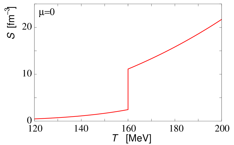
Figure 1: Entropy density as a function of temperature at $\mu=0$. The critical temperature is 160 MeV.

In a forthcoming publication, we will discuss the EoS dependence of physical observables utilizing a realistic lQCD based equation of state, i.e. an EoS with a crossover phase transition at high $T$ and low $\mu$, including the QCD critical point NoAs05 . We are currently in the process of constructing such an EoS, which will correctly capture critical phenomena around the QCD critical point NoAs05 . A simple parameterization of the EoS around the QCD critical point as presented in Brazil_QM is unfortunately insufficient for a description of these phenomena, even though it already provides a marked improvement over currently used equations of state.

II.3 Initial Conditions

The initial conditions for the hydrodynamic calculation need to be determined either by adjusting an appropriate parametrization to data or by utilizing other microscopic transport model predictions for the early non-equilibrium phase of the heavy-ion reaction.

Numerous studies exist for finding the appropriate initial conditions for hydrodynamic models SoHuRu99 ; KoHeHuEsTu01 ; HiNa04 ; HiHeKhLaNa05 ; EsHoNiRuRa05 – usually such an initial condition is given by the parameterization of the spatial distribution of the energy or entropy density and baryon number density at an initial time $\tau_{0}$. A comparison between final particle distributions calculated by the hydrodynamic model and experimental data can then be utilized to fix the values of the parameters for the initial conditions. However, this ansatz is problematic if no experimental data exist to tune the initial conditions. Furthermore, one looses predictive and analytic power by treating the quantities governing the initial conditions as free parameters. Recently there have been several attempts to determine a set of initial conditions not from parameterizations and comparison to data, but via a calculation using the color glass condensate (CGC) model for the initial state HiNa04 ; HiHeKhLaNa05 as well as an approach combining perturbative QCD and the saturation picture EsHoNiRuRa05 . A study of elliptic flow by Hirano et al. has shown that additional dissipation during the early QGP stage is required if an initial condition based on the CGC HiHeKhLaNa05 is used. Another interesting fact which is found in hydrodynamic analyses at RHIC is that thermalization is achieved on very short timescales after the full overlap of the colliding nuclei: none of the hydrodynamic calculations which have successfully addressed RHIC data at the top energy of $\sqrt{s_{NN}}=200$ GeV/nucleon have initial times later than $\tau_{0}\sim 0.6$ fm HuKoHeRuVo01 ; HiTs02 . The physics processes leading to such a rapid thermalization have yet to be unambiguously identified Mr05 – note that hydrodynamics itself cannot address the question of thermalization, since it relies on the assumption of matter being in local thermal equilibrium.

For our calculation we use a simple initial condition which is parameterized based on a combination of wounded nucleon and binary collision scaling JaCo00 ; KoSoHe00 ; KoHeHuEsTu01 . Similar parameterizations have been used in various hydrodynamic models which have been successful in explaining numerous experimental observations at RHIC HuKoHeRuVo01 ; TeLaSh01 ; HiTs02 . We have chosen this common initial condition for our investigation in order to describe the general features of our model and provide a base-line comparison to previous calculations under similar assumptions – in a subsequent publication we shall investigate the sensitivity of our results to particular variations and assumptions regarding the choice of the initial conditions.

We factorize the energy density and baryon number density distributions into longitudinal direction ($H(\eta)$) and the transverse plane ($W(x,y;b)$), which are given by

$$\epsilon(x,y,\eta) = \epsilon_{\rm max}W(x,y;b)H(\eta),$$

$$n_{B}(x,y,\eta) = n_{B{\rm max}}W(x,y;b)H(\eta),$$ (8)

where $\epsilon_{\rm max}$ and $n_{B{\rm max}}$ are parameters which are maximum values of energy density and baryon number density. The longitudinal distribution is parameterized by

$$H(\eta)=\exp\left[-(|\eta|-\eta_{0})/2\sigma^{2}_{\eta}\right]\theta(|\eta|-\eta_{0}),$$ (9)

where parameters $\eta_{0}$ and $\sigma_{\eta}$ are determined by comparison with experimental data of single particle distributions. The function $W(x,y;b)$ on the transverse plane is determined by the superposition of wounded nucleon scaling which is characteristic of “soft” particle production processes and binary collision scaling which is characteristic of “hard” particle production processes HeKo02 . This function is normalized by $W(0,0;0)$. In the wounded nucleon scaling, the density of wounded nucleons is given by

$$\frac{d^{2}N_{\rm WN}}{ds^{2}} = T_{A}(\mbox{\boldmath$b_{A}$})\cdot\left(1-e^{-T_{B}(\mbox{\boldmath$b_{B}$})\sigma}\right)$$ (10)

$$+ T_{B}(\mbox{\boldmath$b_{B}$})\cdot\left(1-e^{-T_{A}(\mbox{\boldmath$b_{A}$})\sigma}\right)\quad,$$

where $\mbox{\boldmath$b_{A}$}=\mbox{\boldmath$s$}+b\cdot e_{x}$ ($\mbox{\boldmath$b_{B}$}=\mbox{\boldmath$s$}-b\cdot e_{x}$), $\sigma$ is the total nucleon-nucleon cross section at Au+Au $\sqrt{s_{NN}}=200$ AGeV and set to 42 mb PHENIX03 . $T_{A}$ is the nuclear thickness function of nucleus $A$,

$$T_{A}(\mbox{\boldmath$s$})=\int dz\rho_{A}(z,\mbox{\boldmath$s$}),$$ (11)

where $\rho_{A}(z,\mbox{\boldmath$s$})$ is given by a Woods-Saxon parameterization of nuclear density,

$$\rho_{A}(r)=\rho_{0}\frac{1}{1+e^{(r-R_{A})/a}}.$$ (12)

In Eq. (12) parameters $a$, $R_{A}$, $\rho_{0}$ are 0.54 fm, 6.38 and 0.1688, respectively PHENIX03 . On the other hand, the distribution of the number of binary collisions is given by

$$\frac{d^{2}N_{\rm BC}}{ds^{2}}=\sigma\cdot T_{A}(\mbox{\boldmath$b_{A}$})T_{B}(\mbox{\boldmath$b_{B}$}).$$ (13)

Then total $W(x,y;b)=w\frac{d^{2}N_{\rm BC}}{ds^{2}}+(1-w)\frac{d^{2}N_{\rm WN}}{ds^{2}}$, where $w$ is the weight factor for binary scaling and is set to 0.6, again utilizing a comparison of experimental data of single particle spectra to our model calculations. Figures 3 and 3 show initial energy density in the longitudinal direction and on the transverse plane for Au+Au $\sqrt{s_{NN}}=200$ GeV central collisions for the case of a hybrid hydro+micro calculation.

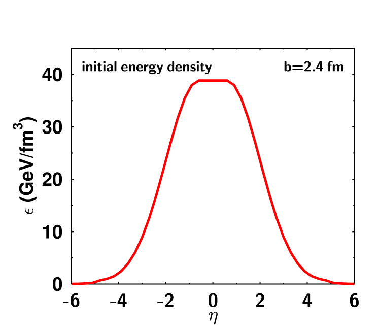
Figure 2: Initial energy density in longitudinal direction at Au+Au $\sqrt{s_{NN}}=200$ GeV central collisions (b=2.4 fm) in the case of Hydro + UrQMD.

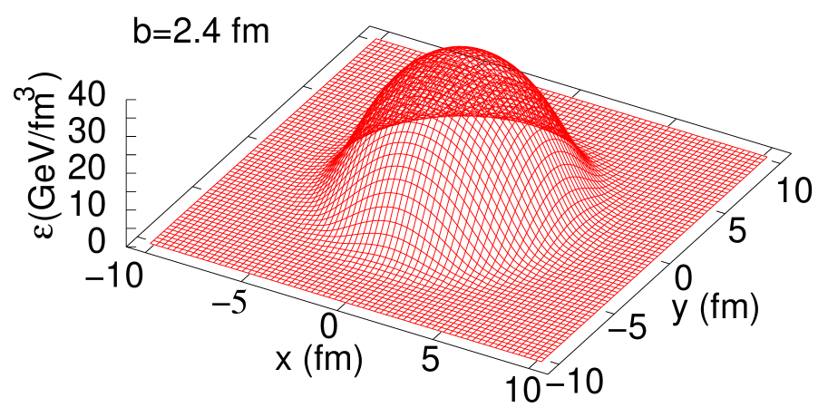
Figure 3: Initial energy density on the transverse plane at Au+Au $\sqrt{s_{NN}}=200$ GeV central collisions (b=2.4 fm) in the case of Hydro + UrQMD.

As a starting point we set initial longitudinal flow to Bjorken’s scaling solution Bjorken:1982qr and neglect initial transverse flow. This is the simplest initial flow profile which will serve as basis for further investigation. For example, Kolb and Rapp discussed the possibility of existence of initial transverse flow which improves the results for $P_{T}$ spectra and reduces the anisotropy in flow KoRa03 , however, at the expense of introducing an additional parameter. Utilizing a parameterized evolution model, it has been pointed out that a Landau-type initial longitudinal compression and re-expansion of matter is favorable for the description of Hanbury-Brown Twiss (HBT) correlation radii Th04 . This suggests that HBT analyses may be a sensitive tool for the determination of the initial longitudinal flow distribution.

In Tab. 3 parameters with which we reproduce single particle spectra at RHIC are listed. The parameters $\eta_{0}$ and $\sigma_{\eta}$ in longitudinal direction are determined mainly by the hadron rapidity distributions and do not strongly affect the transverse momentum distributions. The parameters for the initial conditions need to be optimized separately for the pure hydro and hydro + UrQMD calculations. A comparison between the two sets of initial conditions and possible physics implications can be found in Sec. III. Comparing the initial energy density of our purely hydrodynamic calculation to Ref. KoRa03 in which an initial condition was parameterized in terms of the entropy- and baryon number density (weighted according to the wounded nuclear model by 75% and to the binary collision model by 25 %) we find that our calculation requires a significantly higher initial energy- or entropy density: the maximum value of the entropy density at Au + Au $\sqrt{s_{NN}}=200$ GeV in central collision in KoRa03 is 110 fm^-3, whereas our value of the maximum entropy density is 176 fm^-3. The difference between the two values is most likely due to the treatment of resonance decays – these are explicitly treated in KoRa03 , but are neglected in our case. Note that we consider our purely hydrodynamic calculation solely as a baseline against which we can compare the full hydro+micro model, which of course contains a proper treatment of resonance decays. A third hydrodynamic model implementation described in HiNa04 uses an initial condition purely based on binary collisions. The maximum value of energy density in that calculation (which also treats resonance decays) is found to be $\sim 45$ GeV/fm³, similar to the value we obtain for our hydro+micro calculation.

	$\tau_{0}$	$\epsilon_{\rm max}$	$n_{B{\rm max}}$	$\eta_{0}$	$\sigma_{\eta}$
	(fm/$c$)	(GeV/fm3)	(fm-3)
pure hydro	0.6	55	0.15	0.5	1.5
hydro + UrQMD	0.6	40	0.15	0.5	1.5

Table 3: Parameters for initial conditions of pure hydro and hybrid model.

II.4 Hadronization and the transition to microscopic dynamics

Having specified the initial conditions on the $\tau=\tau_{i}$ hypersurface and the EoS, the hydrodynamical solution in the forward light-cone is determined uniquely. We assume that a freezeout process happens when a temperature in a volume element of fluid is equal to a freezeout temperature $T_{f}$ in the pure 3-D hydrodynamic model. In a hybrid model the transition from macroscopic to microscopic dynamics takes place at a switching temperature $T_{\rm SW}$. The feezeout and switching temperatures respectively can be treated as parameters and determined by comparison to experimental data on single particle spectra.

Due to our use of Lagrangian hydrodynamics, grid points move along the flux of the fluid and are not represented by a fixed coordinate-space lattice any more. Therefore it is non-trivial to estimate of the number of particles flowing through the freezeout hypersurface. Here we start from a simple case BlOl90 : suppose that the number of particles $N(\tau)$ exists in the enclosed volume $\Omega$ that is bounded by a closed surface $S(\tau)$ at time $\tau$. $N(\tau)$ is given by

$$N(\tau)=\int_{\Omega(\tau)}d^{3}rn(\mbox{\boldmath$r$},\tau),$$ (14)

where $n(\mbox{\boldmath$r$},\tau)$ is particle number density. At time $\tau+\delta\tau$, the number of particle $N(\tau)$ changes to

$$\frac{dN}{d\tau}=\int_{\Omega(\tau)}d^{3}r\frac{\partial n}{\partial\tau}+\frac{1}{d\tau}\int_{\delta\Omega}d^{3}rn(\mbox{\boldmath$r$},\tau),$$ (15)

where the volume varies to $\Omega+\delta\Omega$. Utilizing current conservation, $\frac{\partial n}{\partial\tau}+\nabla\cdot\mbox{\boldmath$j$}$ ($j$ is a current of particle), Eq.(15) is rewritten as

$$\frac{dN}{d\tau}=-\int_{S(\tau)}d^{2}s\mbox{\boldmath$j$}\cdot\mbox{\boldmath$n$}+\int_{S(\tau)}d^{2}s\frac{d\zeta}{d\tau}n,$$ (16)

where $n$ is the normal vector of surface element $d^{2}s$ and $d\zeta$ is the distance between the surface of $\Omega(\tau)$ and that of $\Omega(\tau)+\delta\Omega$. In Eq. (16), $dN/d\tau$ is the number of particles which cross the surface $S(\tau)$ during $d\tau$. Then total number of particles through the hypersurface $\Sigma$ which is the set of surfaces $\{S(\tau)\}$,

$$N=\int_{\Sigma}j^{\mu}d\sigma_{\mu},$$ (17)

where $j^{0}=n$, $d\sigma_{0}=d^{3}r$, $d\mbox{\boldmath$\sigma$}=d\tau\cdot d^{2}s\mbox{\boldmath$n$}$. If we write

$$j^{\mu}=\frac{d^{3}P}{E}\frac{g_{h}}{(2\pi)^{3}}\frac{1}{\exp[(P_{\nu}u^{\nu}-\mu_{f})/T_{f}]\pm 1}P^{\mu}$$ (18)

for the current $j^{\mu}$ in Eq. (17), we obtain the Cooper-Frye formula CF

$$E\frac{dN}{d^{3}P}=$$

$$\sum_{h}\frac{g_{h}}{(2\pi)^{3}}\int_{\Sigma}d\sigma_{\mu}P^{\mu}\frac{1}{\exp[(P_{\nu}u^{\nu}-\mu_{f})/T_{f}]\pm 1},$$ (19)

where $g_{h}$ is a degeneracy factor of hadrons and $T_{f}$ and $\mu_{f}$ are the freezeout temperature and chemical potential. In other words we obtain $d\sigma_{\mu}$ by estimating the normal vector on the freezeout hypersurface $\Sigma$. Using Eq. (19), we then can calculate all particle distributions.

In order to pass on the distribution (19) in the macroscopic model to the microscopic model, we first calculate the multiplicities $N_{i}$ for each particle species $i$, by integration of Eq. (19) in which $T_{f}$ and $\mu_{f}$ are changed to the switching temperature $T_{\rm SW}$ and chemical potential $\mu_{\rm SW}$ over space-time ($\tau$, $r$, $\eta$) and momentum space ($P_{T}$, $y$). $N_{i}$ is rounded to an integer value since the hadronic transport model described in the next section deals with real particle degrees of freedom. The distribution (19) divided by $N_{i}$ is used as probability distribution to randomly generate the space-time and momentum-space coordinates for $N_{i}$ hadrons of species $i$. This distribution serves as an input for the hadronic transport model for a single event. The sampling procedure can be repeated to generate a sequence of events as starting points for the microscopic calculation. Each event-sampling produces a different set of space-time and momentum coordinates as input of the microscopic model, however, the total multiplicity for each species $i$ remains constant for a given hydrodynamic switching hyper-surface. In a more realistic calculation, particle number fluctuations should be taken into account as well. The reverse process, absorbing microscopic particles into the hydrodynamic medium is being neglected – it has been shown in Teaney:2001av that for rapidly expanding systems these contributions are negligible.

II.5 Microscopic dynamics: the UrQMD approach

The ensemble of hadrons generated accordingly is then used as initial condition for the microscopic transport model Ultra-relativistic Quantum Molecular Dynamics (UrQMD) uqmdref1 . The UrQMD approach is closely related to hadronic cascade cascade , Vlasov–Uehling–Uhlenbeck vuu and (R)QMD transport models qmd . We shall describe here only the part of the model that is important for the application at hand, namely the evolution of an expanding hadron gas in local equilibrium at a temperature of about $T_{C}\sim 160$ MeV. The treatment of high-energy hadron-hadron scatterings, as it occurs in the initial stage of ultrarelativistic collisions, is not discussed here. A complete description of the model and detailed comparisons to experimental data can be found in uqmdref1 .

The basic degrees of freedom are hadrons modeled as Gaussian wave-packets, and strings, which are used to model the fragmentation of high-mass hadronic states via the Lund scheme lund . The system evolves as a sequence of binary collisions or $2-N$-body decays of mesons, baryons, and strings.

The real part of the nucleon optical potential, i.e. a mean-field, can in principle be included in UrQMD for the dynamics of baryons (using a Skyrme-type interaction with a hard equation of state). However, currently no mean field for mesons (the most abundant hadrons in our investigation) are implemented. Therefore, we have not accounted for mean-fields in the equation of motion of the hadrons. To remain consistent, mean fields were also not taken into account in the EoS on the fluid-dynamical side. Otherwise, pressure equality (at given energy and baryon density) would be destroyed. We do not expect large modifications of the results presented here due to the effects of mean fields, since the “fluid” is not very dense after hadronization and current experiments at SIS and AGS only point to strong medium-dependent properties of mesons (kaons in particular) for relatively low incident beam energies ($E_{lab}\leq 4$ GeV/nucleon) gsikaonen . Nevertheless, mean fields will have to be included in the future.

Binary collisions are performed in a point-particle sense: Two particles collide if their minimum distance $d$, i.e. the minimum relative distance of the centroids of the Gaussians during their motion, in their CM frame fulfills the requirement:

$$d\leq d_{0}=\sqrt{\frac{\sigma_{\rm tot}}{\pi}},\qquad\sigma_{\rm tot}=\sigma(\sqrt{s},\hbox{ type}).$$ (20)

The cross section is assumed to be the free cross section of the regarded collision type ($N-N$, $N-\Delta$, $\pi-N$ …).

The UrQMD collision term contains 53 different baryon species (including nucleon, delta and hyperon resonances with masses up to 2 GeV) and 24 different meson species (including strange meson resonances), which are supplemented by their corresponding anti-particle and all isospin-projected states. The baryons and baryon-resonances which can be populated in UrQMD are listed in table 1, the respective mesons in table 2 – full baryon/antibaryon symmetry is included (not shown in the table), both, with respect to the included hadronic states, as well as with respect to the reaction cross sections. All hadronic states can be produced in string decays, s-channel collisions or resonance decays.

Tabulated and parameterized experimental cross sections are used when available. Resonance absorption, decays and scattering are handled via the principle of detailed balance. If no experimental information is available, the cross section is either calculated via an One-Boson-Exchange (OBE) model or via a modified additive quark model which takes basic phase space properties into account.

In the baryon-baryon sector, the total and elastic proton-proton and proton-neutron cross sections are well known PDG96 . Since their functional dependence on $\sqrt{s_{NN}}$ shows a complicated shape at low energies, UrQMD uses a table-lookup for those cross sections. However, many cross sections involving strange baryons and/or resonances are not well known or even experimentally accessible – for these cross sections the additive quark model is widely used.

As we shall see later, the most important reaction channels in our investigation are meson-meson and meson-baryon elastic scattering and resonance formation. For example, the total meson-baryon cross section for non-strange particles is given by

$$\sigma^{MB}_{tot}(\sqrt{s}) = \sum\limits_{R=\Delta,N^{*}}\langle j_{B},m_{B},j_{M},m_{M}\|J_{R},M_{R}\rangle$$ (21)

$$\times\frac{2S_{R}+1}{(2S_{B}+1)(2S_{M}+1)}$$

$$\times\frac{\pi}{p^{2}_{CMS}}\,\frac{\Gamma_{R\rightarrow MB}\Gamma_{tot}}{(M_{R}-\sqrt{s})^{2}+\frac{\Gamma_{tot}^{2}}{4}}$$

with the total and partial $\sqrt{s}$-dependent decay widths $\Gamma_{tot}$ and $\Gamma_{R\rightarrow MB}$. The full decay width $\Gamma_{tot}(M)$ of a resonance is defined as the sum of all partial decay widths and depends on the mass of the excited resonance:

$$\Gamma_{tot}(M)\,=\,\sum\limits_{br=\{i,j\}}^{N_{br}}\Gamma_{i,j}(M)\quad.$$ (22)

The partial decay widths $\Gamma_{i,j}(M)$ for the decay into the final state with particles $i$ and $j$ is given by

$$\Gamma_{i,j}(M) = \Gamma^{i,j}_{R}\frac{M_{R}}{M}\left(\frac{\langle p_{i,j}(M)\rangle}{\langle p_{i,j}(M_{R})\rangle}\right)^{2l+1}$$ (23)

$$\times \frac{1.2}{1+0.2\left(\frac{\langle p_{i,j}(M)\rangle}{\langle p_{i,j}(M_{R})\rangle}\right)^{2l}}\quad,$$

here $M_{R}$ denotes the pole mass of the resonance, $\Gamma^{i,j}_{R}$ its partial decay width into the channel $i$ and $j$ at the pole and $l$ the decay angular momentum of the final state. All pole masses and partial decay widths at the pole are taken from the Review of Particle Properties PDG96 . $\Gamma_{i,j}(M)$ is constructed in such a way that $\Gamma_{i,j}(M_{R})=\Gamma^{i,j}_{R}$ is fulfilled at the pole. In many cases only crude estimates for $\Gamma^{i,j}_{R}$ are given in PDG96 – the partial decay widths must then be fixed by studying exclusive particle production in elementary proton-proton and pion-proton reactions. Therefore, e.g., the total pion-nucleon cross section depends on the pole masses, widths and branching ratios of all $N^{*}$ and $\Delta^{*}$ resonances listed in table 1. Resonant meson-meson scattering (e.g. $\pi+\pi\to\rho$ or $\pi+K\to K^{*}$) is treated in the same formalism.

In order to correctly treat equilibrated matter belkbrand (we repeat that the hadronic matter with which UrQMD is being initialized in our approach is in local chemical and thermal equilibrium), the principle of detailed balance is of great importance. Detailed balance is based on time-reversal invariance of the matrix element of the reaction. It is most commonly found in textbooks in the form:

$$\sigma_{f\rightarrow i}\,=\,\frac{\vec{p}_{i}^{2}}{\vec{p}_{f}^{2}}\frac{g_{i}}{g_{f}}\sigma_{i\rightarrow f}\quad,$$ (24)

with $g$ denoting the spin-isospin degeneracy factors. UrQMD applies the general principle of detailed balance to the following two process classes:

1. Resonant meson-meson and meson-baryon interactions: Each resonance created via a meson-baryon or a meson-meson annihilation may again decay into the two hadron species which originally formed it. This symmetry is only violated in the case of three- or four-body decays and string fragmentations, since N-body collisions with (N$>2$) are not implemented in UrQMD.

2. Resonance-nucleon or resonance-resonance interactions: the excitation of baryon-resonances in UrQMD is handled via parameterized cross sections which have been fitted to data. The reverse reactions usually have not been measured - here the principle of detailed balance is applied. Inelastic baryon-resonance de-excitation is the only method in UrQMD to absorb mesons (which are bound in the resonance). Therefore the application of the detailed balance principle is of crucial importance for heavy nucleus-nucleus collisions.

Equation (24), however, is only valid in the case of stable particles with well-defined masses. Since in UrQMD detailed balance is applied to reactions involving resonances with finite lifetimes and broad mass distributions, equation (24) has to be modified accordingly. For the case of one incoming resonance the respective modified detailed balance relation has been derived in danielewicz91a . Here, we generalize this expression for up to two resonances in both, the incoming and the outgoing channels.

The differential cross section for the reaction $(1\,,\,2)\rightarrow(3\,,\,4)$ is given by:

$${\rm d}\sigma_{12}^{34}\,=\,\frac{|{\cal M}|^{2}}{64\pi^{2}s}\,\frac{p_{34}}{p_{12}}\,{\rm d\Omega}\,\prod_{i=3}^{4}\delta(p_{i}^{2}-M_{i}^{2}){\rm d}p_{i}^{2}\quad,$$ (25)

here the $p_{i}$ in the $\delta$-function denote four-momenta. The $\delta$-function ensures that the particles are on mass-shell, i.e. their masses are well-defined. If the particle, however, has a broad mass distribution, then the $\delta$-function must be substituted by the respective mass distribution (including an integration over the mass):

$${\rm d}\sigma_{12}^{34}\,=\,\frac{|{\cal M}|^{2}}{64\pi^{2}s}\,\frac{1}{p_{12}}\,{\rm d\Omega}\,\prod_{i=3}^{4}p_{34}\cdot\frac{\Gamma}{\left(m-M_{i}\right)^{2}+\Gamma^{2}/4}\frac{{\rm d}m}{2\pi}\,.$$ (26)

Incorporating these modifications into equation (24) and neglecting a possible mass-dependence of the matrix element we obtain:

$$\frac{{\rm d}\sigma_{34}^{12}}{{\rm d}\Omega} = \frac{\langle p_{12}^{2}\rangle}{\langle p_{34}^{2}\rangle}\,\frac{(2S_{1}+1)(2S_{1}+1)}{(2S_{3}+1)(2S_{4}+1)}$$ (27)

$$\times \sum_{J=J_{-}}^{J_{+}}\langle j_{1}m_{1}j_{2}m_{2}\|JM\rangle\,\frac{{\rm d}\sigma_{12}^{34}}{{\rm d}\Omega}\,.$$

Here, $S_{i}$ indicates the spin of particle $i$ and the summation of the Clebsch-Gordan-coefficients is over the isospin of the outgoing channel only. For the incoming channel, isospin is treated explicitly. The summation limits are given by:

$$J_{-} = \max\left(|j_{1}-j_{2}|,|j_{3}-j_{4}|\right)$$ (28)

$$J_{+} = \min\left(j_{1}+j_{2},j_{3}+j_{4}\right)\quad.$$ (29)

The integration over the mass distributions of the resonances in equation (27) has been denoted by the brackets $\langle\rangle$, e.g.

$$p_{3,4}^{2}\Rightarrow\langle p_{3,4}^{2}\rangle$$

$$=\,\int\int p_{CMS}^{2}(\sqrt{s},m_{3},m_{4})\,A_{3}(m_{3})\,A_{4}(m_{4})\,{\rm d}m_{3}\;{\rm d}m_{4}$$

with the mass distribution $A_{r}(m)$ given by a free Breit-Wigner distribution with a mass-dependent width according to equation (22):

$$A_{r}(m)\,=\,\frac{1}{N}\frac{\Gamma(m)}{(m_{r}-m)^{2}+\Gamma(m)^{2}/4}$$ (30)

with

$$\lim_{\Gamma\rightarrow 0}A_{r}(m)=\delta(m_{r}-m)\,,$$

and the normalization constant

$$N\,=\,\int\limits_{-\infty}^{\infty}\frac{\Gamma(m)}{(m_{r}-m)^{2}+\Gamma(m)^{2}/4}\,{\rm d}m\,.$$ (31)

Alternatively one can also choose a Breit-Wigner distribution with a fixed width, the normalization constant then has the value $N=2\pi$.

The most frequent applications of equation (27) in UrQMD are the processes $\Delta_{1232}\,N\to N\,N$ and $\Delta_{1232}\,\Delta_{1232}\to N\,N$.

III Results

III.1 Modeling of the entire reaction dynamics in three-dimensional hydrodynamics

The purpose of this section is to establish a baseline against which we can later compare the results of our hybrid macro+micro model. In addition we wish to demonstrate that our novel implementation of the 3+1 dimensional relativistic hydrodynamic model, utilizing a Lagrangian grid, is capable of reproducing the results of previous hydrodynamic calculations. Many of these previous calculations found in the literature have focused on one or two particular observables – here we wish to conduct a consistent analysis of all relevant single-particle distributions which can be addressed by a hydrodynamic calculation.

In order to obtain qualitative results which are comparable to experimental data, we have to determine the parameters of the initial conditions. This is accomplished by adjusting the parameters to fit the single particle spectra for the most central Au+Au collisions at $\sqrt{s_{NN}}=200$ GeV.

First we show the behavior of isentropic trajectories in the $T-\mu$ plane for Au+Au $\sqrt{s_{NN}}=200$ GeV central collisions in Fig. 4. The dotted line stands for the phase boundary between the QGP and the hadronic phase (Note that due to small baryochemical potentials, the phase boundary is an almost flat line at $T_{C}=160$ MeV). Apart from the central cell, we also investigate the isentropic trajectory of a cell close to the surface of the initially produced QGP. Whereas the isentropic trajectory of the central cell located at $(0,0,0)$ starts in the QGP phase (solid line), the cell at the initial surface of the QGP (dashed line) only exhibits an evolution from the mixed phase to the hadronic phase. Both trajectories are terminated at freezeout temperature, $T_{\rm f}=110$ MeV.

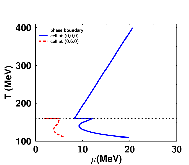
Figure 4: The isentropic trajectories on $T-\mu$ plane. Solid (Dashed) line stands for the behavior of sell which is located at $(x,y,\eta)=(0,0,0)(=(0,6,0))$ at initial time. Dotted line represents phase boundary.

Figure 6 shows the $P_{T}$ spectra of $\pi$, $K$ and $p$ in Au + Au at $\sqrt{s_{NN}}=200$ GeV for central collisions. Our calculation succeeds in reproducing the $\pi$ spectra measured by the PHENIX collaboration PHENIX_PT up to $P_{T}\sim 2$ GeV. However, due to the model assumption of chemical equilibrium up to the (low) kinetic freezeout temperature, we fail to obtain the correct normalization and hadron ratios, even though the shape of the $P_{T}$ spectra of $p$ and multistrange baryons (shown in Fig. 6) is close to experimental data. In order to obtain the proper normalization for the $p$ spectra and match the experimentally measured hadron ratios we adopt a procedure outlined in Ref. hadron-ratio , which renormalizes the $P_{T}$ spectra using the $p$ to $\pi$ ratio at the critical temperature to fix the normalization of the proton spectra. It is straightforward to extend this procedure to hyperons and multi-strange baryons as well, even though we choose to show the real, unrenormalized, result for the multi-strange baryons in Fig. 6 to elucidate the situation prior to renormalization.

The need for renormalizing the $p$ spectra suggests that the assumption of a continuous chemical equilibrium until kinetic freezeout is not realistic and that an improved treatment of the freeze-out process is required. One method to deal with the separation of chemical and thermal freeze-out is the partial chemical equilibrium model (PCE) HiTs02 ; Te02 ; KoRa03 : below a chemical freeze-out temperature $T_{ch}$ one introduces a chemical potential for each hadron whose yield is supposed to be frozen-out at that temperature. The PCE approach can account for the proper normalization of the spectra, however, it fails to reproduce the transverse momentum and mass dependence of the elliptic flow PHENIX_white . In section III.2, we shall utilize our hybrid hydro+micro model to decouple chemical and kinetic freeze-out. In these hybrid approaches BaDu00 ; TeLaSh01 ; HiHeKhLaNa05 the freeze-out occurs sequentially as a result of the microscopic evolution and flavor degrees of freedom are treated explicitly through the hadronic cross sections of the microscopic transport, leading to the proper normalization of all hadron spectra.

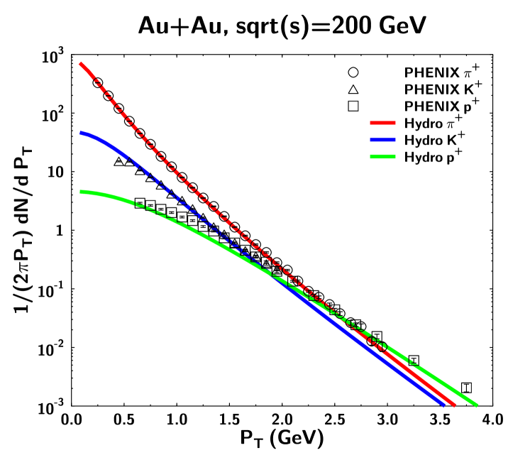
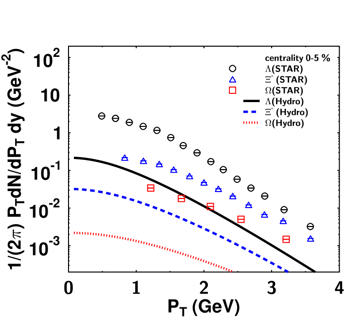
Figure 5: $P_{T}$ spectra for $\pi^{+}$, $K^{+}$, $p$ at central collisions with PHENIX data PHENIX_PT . For proton we rescale our result using the ration at chemical temperature (See the text).

Figure 6: $P_{T}$ spectra for multistrange baryons at central collisions with STAR data STAR_strange1 . In this calculation (pure hydro) the additional procedure for normalization is not done.

In Fig. 7 the centrality dependence of $P_{T}$ spectra for $\pi^{+}$ is shown. The impact parameters are set to $b=$2.4, 4.5, 6.3, 7.9 fm corresponding to 0-6, 10-15, 15-20, 20-30 % centrality, respectively. These values are estimated via the number of nucleon-nucleon binary collisions and the number of participant nucleons in Ref. PHENIX_PT . The centrality dependence is determined simply by the collision geometry – no additional parameter is necessary for our finite impact parameter collision calculations in Sec. II.3. Our results are consistent with the experimental data PHENIX_PT in the low transverse momentum region ($0<P_{T}<1$ GeV) for all centralities. We observe that in peripheral collisions the difference between experimental data and our calculations appears at lower $P_{T}$ compared to central collisions. This difference is indicative of the diminished importance of the soft, collective, physics described by hydrodynamics compared to the contribution of jet-physics in peripheral events.

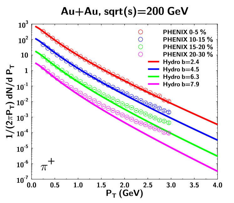
Figure 7: Centrality dependence of $P_{T}$ spectra of $\pi^{+}$ with PHENIX data PHENIX_PT . The $P_{T}$ spectra at 10–15 %, 15–20 % and 20–30 % are divided by 5, 25 and 200, respectively.

Figure 8 shows the centrality dependence of the pseudorapidity distribution of charged hadrons compared to PHOBOS data PHOBOS_eta . The parameters of our initial condition in the longitudinal direction ($\sigma_{\eta}$, $\eta_{0}$) have been determined by fitting the data for the most central collisions, no additional parameter is needed to fix the initial conditions for non-central collisions, since they result solely from the collision geometry. The impact parameters for our calculation are set to $b=$2.4, 4.5, 6.3 and 7.9 fm corresponding to 0-6 %, 6-15 %, 15-25 % and 25-35 % centrality, respectively PHOBOS_eta . We find good agreement of our results with the experimental data not only at mid rapidity but also at forward and backward rapidities, suggesting that the pure 3-D hydrodynamic model can explain the charged hadron multiplicity distribution in a wide range of rapidity. This observation is consistent with results of other pure hydrodynamic models Hi01 ; HiTs02 ; Morita utilizing different computational methods. However, as we show it later, the hydrodynamic calculation overestimates the elliptic flow at forward/backward rapidity, indicating that the rapidity distribution is rather insensitive to the details of the expansion dynamics.

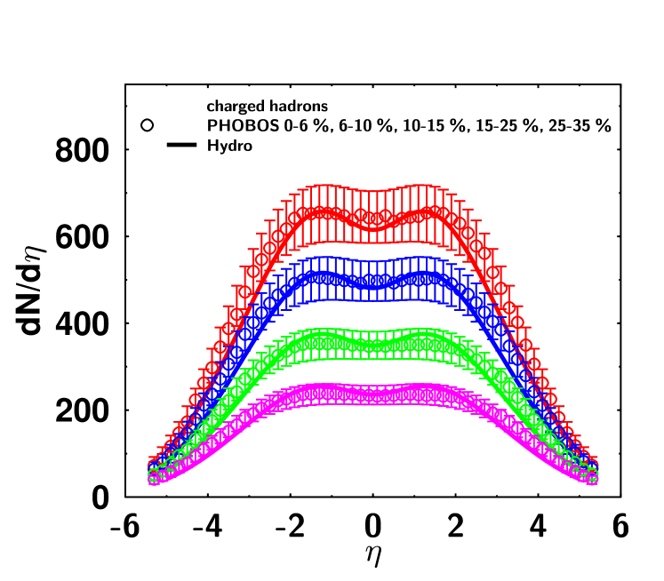
Figure 8: Centrality dependence of pseudorapidity distribution with PHOBOS data PHOBOS_eta . Impact parameters in the hydrodynamic model are 2.4, 4.5, 6.3, 7.5 fm from central to peripheral collisions.

Having fixed all parameters of our initial condition utilizing the $P_{T}$ spectra and (pseudo)rapidity distributions in the most central collisions we now apply our hydrodynamic model to other physical observables using these parameters.

The elliptic flows as a function of $P_{T}$ in 5-10 % and 10-20 % most central collisions are shown in Fig. 9 (a) and (b) together with STAR data STAR_v2 at mid rapidity. We set the impact parameter in our hydrodynamic calculation to 4.5 fm (6.3 fm) for the 5-10 % (10-20 %) data. In the case of the 5-10 % most central events , we obtain reasonable agreement to the data for $\pi$ and $p$. On the other hand, in the 10-20 % centrality bin our hydrodynamical calculation overpredicts the elliptic flow compared to experimental data. Especially for protons, the deviation between calculation and experimental data is fairly large – this trend has already been observed in Hirano:2002ds .

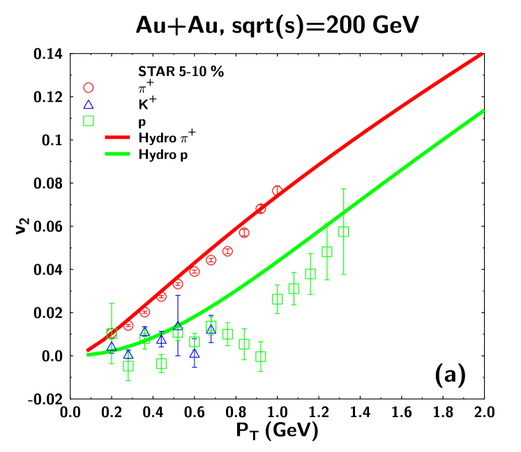
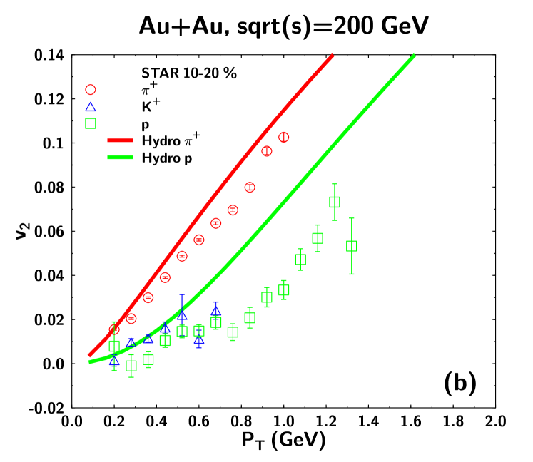
Figure 9: Elliptic flow as a function of $P_{T}$ with STAR data STAR_v2 in centrality 5-10 % (a) and in centrality 10-20 % (b). Impact parameters in hydrodynamic calculations are 4.5 fm (a) and 6.3 fm (b).

Figure 10 shows the elliptic flow as a function of $\eta$ in central (3-15 %) and mid central collisions (15-25 %). In both cases our hydrodynamic model calculations overestimate the elliptic flow at forward and backward rapidities, similar to results shown in Ref. HiTs02 . At large forward and backward rapidities the assumptions of a perfect hydrodynamic model such as local equilibrium, vanishing mean free path and neglect of viscosity effect apparently are no longer valid. The deviations at forward and backward rapidities between experimental data and calculated results increase with the impact parameter, indicating a decrease of the volume in which hydrodynamic limit is achieved.

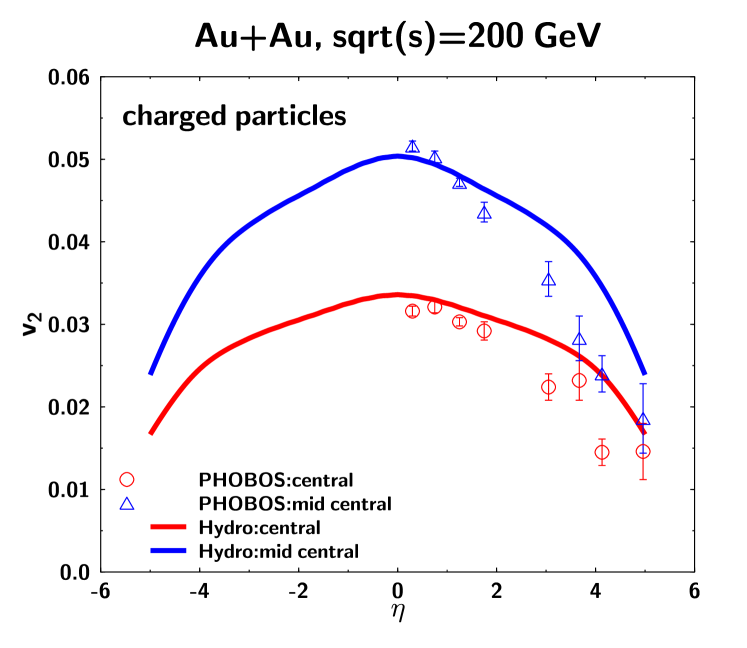
Figure 10: Elliptic flow as a function of $\eta$ with PHOBOS experimental data PHOBOS_v2_eta for central (3-15 %) and mid central collisions (15-25 %). Impact parameters are set to 4.5 (central) and 6.3 (mid central) fm, respectively.

Summarizing this section, we have applied our ideal 3D RFD model to Au+Au collisions at the top RHIC energy. A set of parameters for the initial conditions has been determined which allows for the simultaneous description of $\pi$, $K$ and $p$ $P_{T}$ spectra, the charged hadron rapidity distribution and the $P_{T}$ as well as rapidity dependence of the elliptic flow coefficient $v_{2}$ for $\pi$ and $p$. Without any additional parameters the 3D RFD model is capable of describing the centrality dependence of the $P_{T}$ spectra and charged hadron rapidity distribution as well.

However, our analysis also has demonstrated a couple of deficits of the ideal 3D RFD approach – many of which are already well-known and have been discussed in the literature before Hirano:2002ds ; Kolb:2003dz :

• the centrality dependence of the elliptic flow coefficient $v_{2}$ as a function of $P_{T}$ is not well described,

• the width of the $v_{2}$ vs. $\eta$ distribution is too broad compared to data,

• $p$ and multistrange particle spectra need to be normalized by hand in order to account for the separation of chemical and kinetic freeze-out,

• the hydrodynamic approach is only of limited applicability for small systems (i.e. large impact parameters) and large $P_{T}$ (hard physics).

In the following section, we shall use the 3D RFD calculation as a baseline to determine the effects of an improved treatment of the hadronic phase in the framework of the hydro+micro approach.

III.2 Application of the hydro+micro approach

As in the previous subsection, we first determine the parameters of the initial conditions in Sec. II.3 by fitting the single particle spectra in the most central centrality bin. Table 3 shows the parameters for both, the pure 3D RFD initial condition as well as the hydro+micro initial condition. The main difference we find between the two is in the maximum value of initial energy density. The large difference between the two initial energy densities can be explained by our omission of resonance decays in the pure hydrodynamic calculation and to a lesser extent by the dissipative corrections present in the hydro+micro calculation. Both effects result in additional particle production, leading to a smaller initial energy- and entropy-density necessary to describe the final particle multiplicities.

We set the switching temperature $T_{\rm SW}$ to 150 MeV. This allows for a brief period of hydrodynamic evolution in the hadronic phase to account for multi-particle collisions which can occur at large densities and temperatures in the hadronic phase close to the phase-boundary rapp ; leupold . The dependence of hadronic observables on $T_{\rm SW}$, such as the mean transverse momentum $\langle P_{T}\rangle$ of the different hadron species, has been investigated in BaDu00 – our choice of 150 MeV conforms to the lower bound of the allowed range for $T_{\rm SW}$.

Figure 11 shows the $P_{T}$ spectra of $\pi^{+}$, $K$ and $p$ at $\sqrt{s_{NN}}=200$ GeV central collisions. The most compelling feature, compared to the pure 3D RFD calculation, is that the hydro+micro approach is capable of accounting for the proper normalization of the spectra for all hadron species without any additional correction as is performed in the pure hydrodynamic model. The introduction of a realistic freezeout process provides therefore a natural solution to the problem of separating chemical and kinetic freeze-out in a pure hydrodynamic approach.

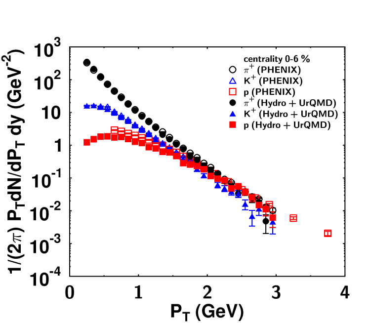
Figure 11: $P_{T}$ spectra for $\pi^{+}$, $K^{+}$ and $p$ at central collisions with PHENIX data PHENIX_PT . The poins are NOT renormalized.

In Fig. 12 centrality dependence of $P_{T}$ spectra of $\pi^{+}$ is shown. The impact parameter for each centrality is determined in the same way as in the pure hydrodynamic calculation. The separation between model results and experiment appears at lower transverse momentum in peripheral collisions compared to central collisions, just as in the pure hydrodynamic calculation. The 3D hydro + micro model does not provide any improvement for this behavior, since the hard physics high $P_{T}$ contribution to the spectra occurs at early reaction times before the system has reached the QGP phase and is therefore neither included in the pure 3D RFD calculation nor in the hydro+micro approach.

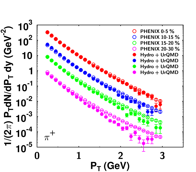
Figure 12: Centrality dependence of $P_{T}$ spectra of $\pi^{+}$ with PHENIX data PHENIX_PT . The $P_{T}$ spectra at 10–15 %, 15–20 % and 20–30 % are divided by 5, 25 and 200, respectively.

Figure 13 shows the centrality dependence of the pseudorapidity distribution of charged hadrons compared to PHOBOS data PHOBOS_eta . Solid circles stand for model results and open circles denote data taken by the PHOBOS collaboration PHOBOS_eta . The impact parameters are set to $b=2.4,4.5,6.3,7.9$ fm for 0-6 %, 6-15 %, 15-25 % and 25-35 % centralities, respectively. Our results are consistent with experimental data over a wide pseudorapidity region. We observe a small deviation around $|\eta|~{}\sim 3$, which may be improved by tuning the parameter $\sigma_{\eta}$ (here we have chosen the same value as for the pure RFD calculation). There is no distinct difference between 3-D ideal RFD model and the hydro + UrQMD model in the centrality dependence of the psuedorapidity distribution, indicating that the shape of psuedorapidity distribution is insensitive to the detailed microscopic reaction dynamics of the hadronic final state.

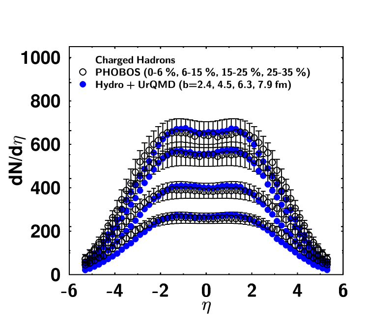
Figure 13: Centrality dependence of pseudorapidity distribution of charged particles with PHOBOS data PHOBOS_eta . Impact parameters in a calculation are 2.4 (0-6 %), 4.5 (6-10 %), 6.3 (10-15 %), 7.5 fm (25-35 %).

In Fig. 14 we analyze the $P_{T}$ spectra of multistrange particles. Our results show good agreement with experimental data for $\Lambda$, $\Xi$, $\Omega$ for centralities 0–5 % and 10–20 %. In this calculation the additional procedure for normalization is not needed. Recent experimental results suggest that at thermal freezeout multistrange baryons exhibit less transverse flow and a higher temperature closer to the chemical freezeout temperature compared to non- or single-strange baryons STAR_strange1 ; STAR_strange2 . This behavior can be understood in terms of the flavor dependence of the hadronic cross section, which decreases with increasing strangeness content of the hadron. The reduced cross section of multi-strange baryons leads to a decoupling from the hadronic medium at an earlier stage of the reaction, allowing them to provide information on the properties of the hadronizing QGP less distorted by hadronic final state interactions vanHecke:1998yu ; Dumitru:1999sf . It should be noted that the analogous behavior has already been observed in experiments at the CERN-SPS sps_multistrange . Later in this section we will discuss the reaction dynamics of multi-strange baryons in greater detail by analyzing the baryon collision number and freezeout time distributions as well as their collision rates.

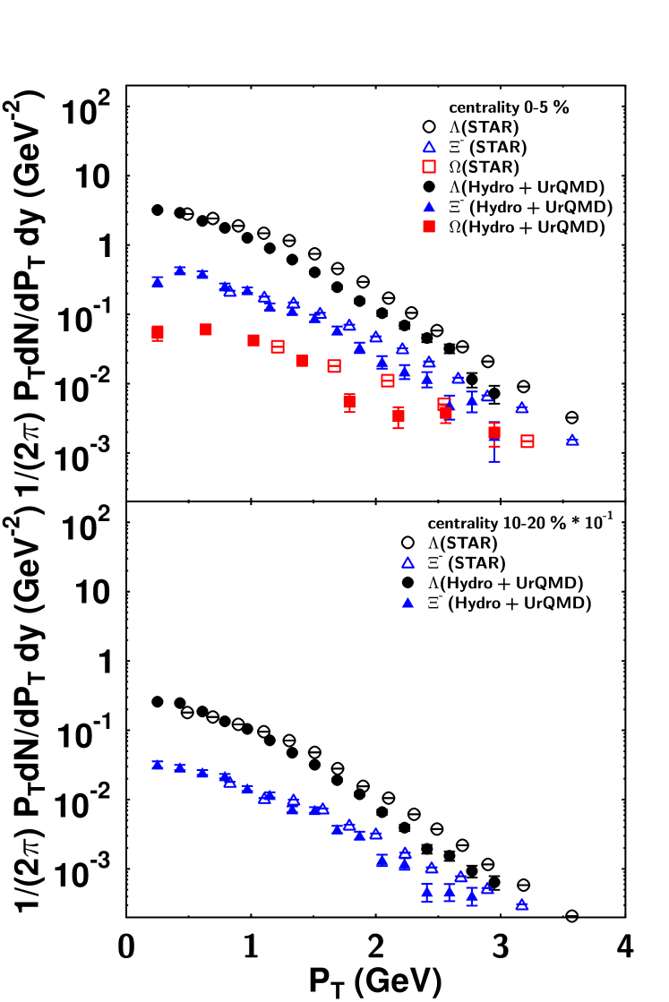
Figure 14: $P_{T}$ spectra of multi-strange particles at centralities 0–5 % and 10–20 % with STAR data STAR_strange1 .

In Fig. 15 the mean transverse momentum $\langle P_{T}\rangle$ as a function of hadron mass is shown. Open symbols denote the value at $T_{\rm sw}=150$ MeV, corrected for hadronic decays. Not surprisingly, in this case the $\langle P_{T}\rangle$ follow a straight line, suggesting a hydrodynamic expansion. However if hadronic rescattering is taken into account (solid circles) the $\langle P_{T}\rangle$ do not follow the straight line any more: the $\langle P_{T}\rangle$ of pions is actually reduced by hadronic rescattering (they act as a heat-bath in the collective expansion), whereas protons actually pick up additional transverse momentum in the hadronic phase. RHIC data by the STAR collaboration is shown via the solid triangles – overall the proper treatment of hadronic final state interactions significantly improves the agreement of the model calculation with the data.

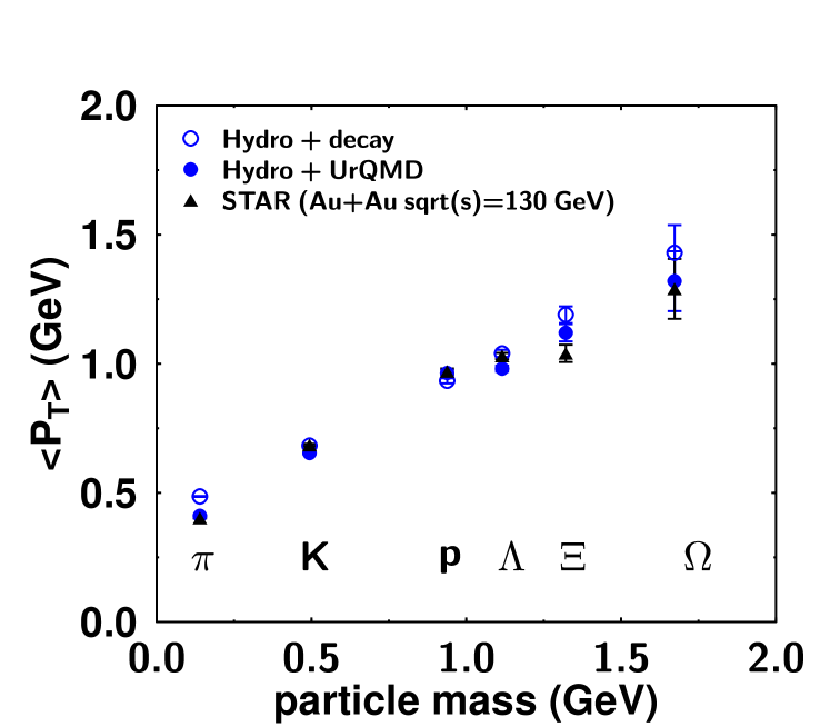
Figure 15: Mean $P_{T}$ as a function of mass. Open circle symbols stand for hydro + decay, solid circle symbols stand for hydro + UrQMD and solid triangle stand for STAR data (Au+Au $\sqrt{s_{NN}}=130$ GeV).

Let us now investigate the effect of resonance decays and hadronic rescattering on the pion and baryon transverse momentum spectra: Figure 16 shows the $P_{T}$ spectrum for $\pi^{+}$ at $T_{\rm sw}=150$ MeV (solid line, uncorrected for resonance decays) as well as the final spectrum after hadronic rescattering and resonance decays, labeled as Hydro+UrQMD (solid symbols). In addition the open symbols denote a calculation with the resonance decay correction performed at $T_{\rm sw}$, which we label as Hydro+decay. The difference between the solid line and open symbols therefore directly quantifies the effect of resonance decays on the spectrum, which is most dominant in the low transverse momentum region $P_{T}<1$ GeV Furthermore, the comparison between open symbols and solid symbols quantifies the effect of hadronic rescattering: pions with $P_{T}>1$ GeV lose momentum via these final state interactions, resulting in a steeper slope.

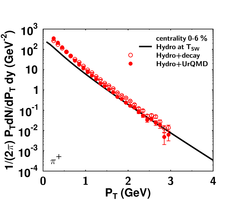
Figure 16: $P_{T}$ spectra of $\pi^{+}$ from hydro at switching temperature (solid line), hydro+decay (open symbols) and hydro + UrQMD (solid symbols) at central collision.

Figure 17 shows a likewise analysis for baryons (p, $\Lambda$, $\Xi$ and $\Omega$). We note that in contrast to SPS energies BaDu00 , there is very little effect on the spectra due to hadronic rescattering - even for protons which rescatter 8 – 10 times at mid-rapidity. Only at low transverse momenta the multiple scatterings of the protons (predominantly with pions) manifests itself in a slight flattening of the $P_{T}$ distribution of the protons, giving rise to a slight increase in their radial flow. This phenomenon has been discussed in Ref. BaDu00 and is commonly referred to as ‘pion wind’.

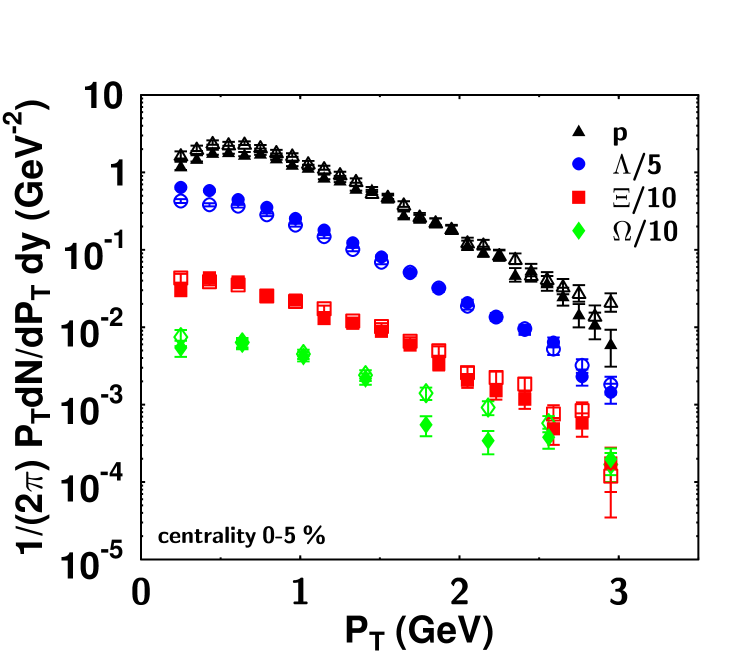
Figure 17: $P_{T}$ spectra of baryons from hydro+decay (open symbols) and hydro + UrQMD (solid symbols) at centrality 0–5 %.

Figure 18 shows the distribution of the number of collisions which particles suffer in the hadronic phase at $b=2.4$, 4.5, 6.3 fm. The distributions for protons and lambdas are very broad, indicating a large amount of rescattering taking place in the hadronic phase. Around mid-rapidity protons rescatter on average 10 times for central and semi-central impact parameters and lambdas rescatter 7-8 times (See also Fig. 19.). However, the average number of collision of multistrange baryons is less than half of those for protons and $\Lambda$’s, as is to be expected due to the decrease of the hadronic cross section with increasing strangeness content of the hadron. We note that the collision number distributions change significantly as a function of centrality – for large impact parameters the high-$n_{\rm coll}$ tail of the distribution exhibits a much steeper drop as a function of $n_{\rm coll}$.

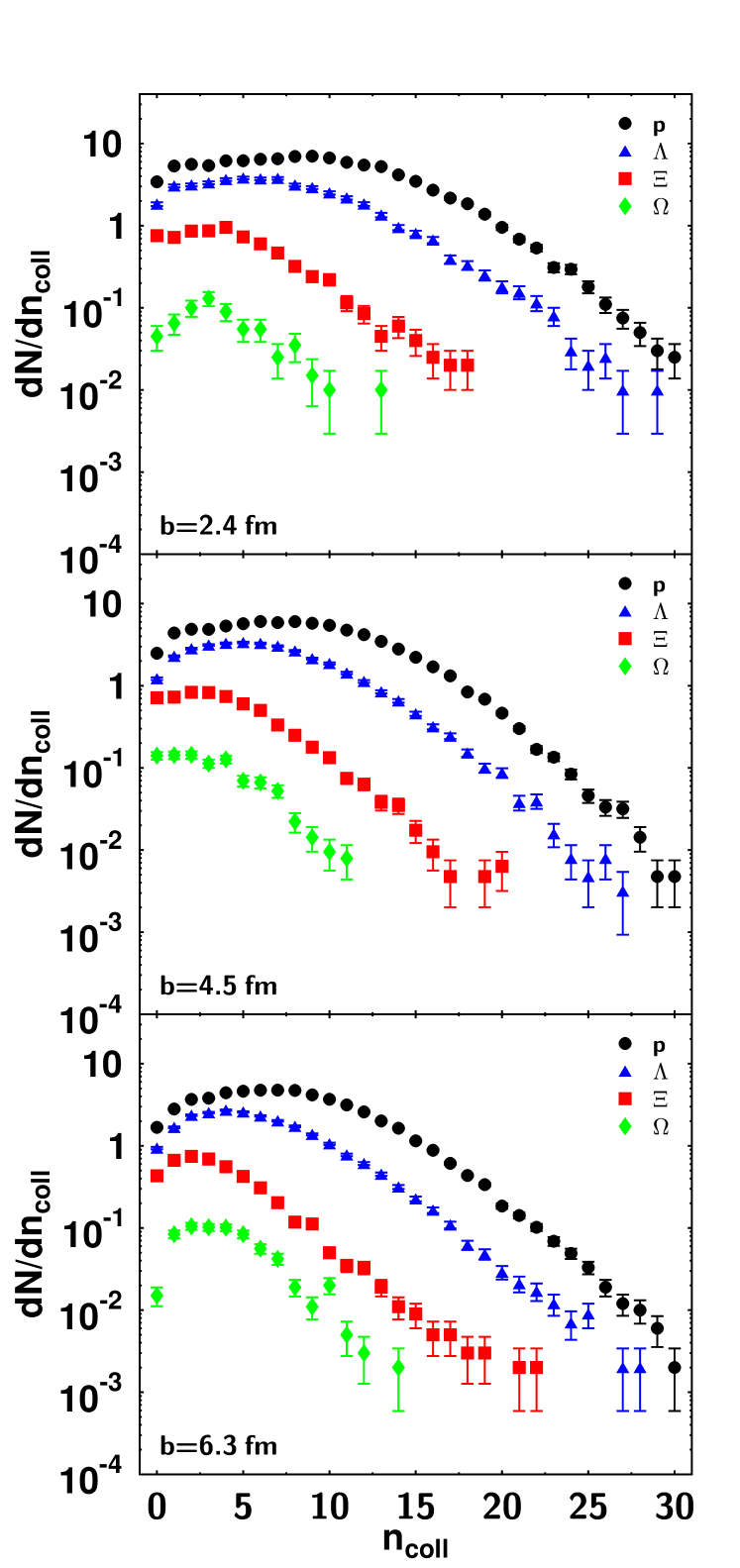
Figure 18: The impact parameter dependence of distribution of number of collisions for $p$, $\Lambda$, $\Xi$, $\Omega$.

The pseudo-rapidity dependence of the number of hadronic rescatterings for different baryon species is analyzed in Fig. 19, which shows the number of collisions of $p$, $\Lambda$, $\Xi$ and $\Omega$ as a function of $\eta$ at $b=2.4$, 4.5 and 6.3 fm. The distributions appear to be similar to that of the particle yield psuedorapidity distribution. At midrapidity we find a plateau region extending from $\eta=-3$ to 3, followed by a steep drop-off to forward and backward rapidities. The flavor dependence of the average collision numbers is again clearly seen, even though we would like to point out that the shapes of the different distributions is very similar. The large plateau region indicates the rapidity domain in which interacting matter can be found and in which the application of thermodynamic concepts is viable.

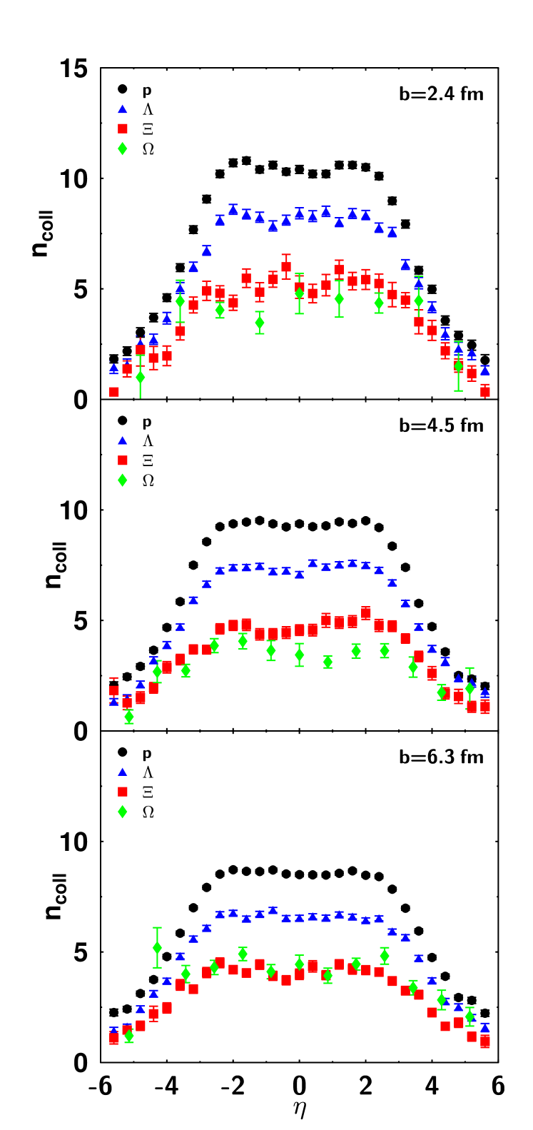
Figure 19: The impact parameter dependence of distribution of number of collisions as a function of $\eta$ for $p$, $\Lambda$, $\Xi$ and $\Omega$.

Figure 20 depicts the freezeout time distribution of $\pi$, $K$, $p$, $\Lambda$, $\Xi$ and $\Omega$ at midrapidity for $b=2.4$, 4.5, 6.3 fm. The freezeout time distribution of $\pi$ and $K$ has a peak around $\tau\sim 19$ ($<20$ fm), while the peak of $p$ and $\Lambda$ freezeout time distribution is shifted to later times. We also note that the freezeout time of multistrange baryons is much smaller than that of other particles. The freezeout times are in general determined by the amount of hadronic rescattering suffered by the different hadron species – our analysis indicates that (a) hadronic freeze-out is strongly species dependent, and (b) even for a particular species, the freeze-out distribution is broad and it is therefore nearly impossible (or at least extremely ambiguous) to define a precise freeze-out time for a given hadron species.

This figure again supports the finding that multistrange baryons are produced with few interactions right after hadronization and freeze-out early vanHecke:1998yu ; Dumitru:1999sf , indications of which have been observed by the STAR collaboration STAR_strange1 ; STAR_strange2 . Given the broad freeze-out time distributions it is very difficult to quantify the overall duration of the heavy-ion reaction – a possible criterion would be the drop-off of the number of freezing out particles per unit time and rapidity below 1 – which would put the overall duration of the reaction to approximately 30 fm/c.

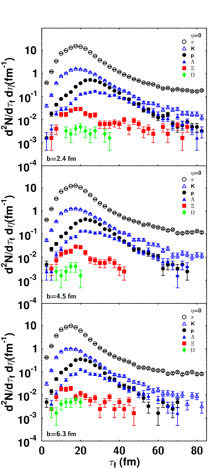
Figure 20: The freezeout time distribution of $\pi$, $K$, $p$, $\Lambda$, $\Xi$ and $\Omega$ at mid rapidity for $b=2.4$, 4.5, 6.3 fm.

In Fig. 21 we study the effect hadronic rescattering has on the duration of the freeze-out process by comparing a calculation terminated at $T_{\rm sw}$ without hadronic rescattering (open symbols) to one including the full hadronic final state interactions (solid symbols). If we terminate at $T_{\rm sw}$, most hadrons freezeout around 10 fm/c, reflecting the lifetime of the deconfined phase in our calculation (the tails of the distribution stem from the decays of long-lived resonances). The inclusion of hadronic rescattering shifts the peak of the freezeout distribution to larger freezeout times ($\tau_{f}\sim 20-30$), providing us with an estimate on the lifetime of the hadronic phase around 10-20 fm/c. Note that this estimate is subject to the same systematic uncertainties discussed previously in the context of the overall lifetime of the system.

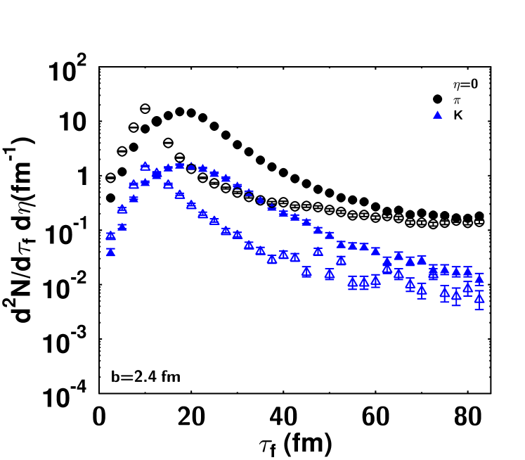
Figure 21: The freezeout time distribution of mesons for hydro+decay (open symbols) and hydro + UrQMD (solid symbols) at mid rapidity in the case of central collision.

The findings discussed in the context of the previous figure for pions and kaons are confirmed by analyzing baryons in the same fashion, which is shown in Fig. 22: here the top frame contains the analysis terminated at $T_{\rm sw}$ and the bottom frame contains the calculation including full hadronic rescattering.

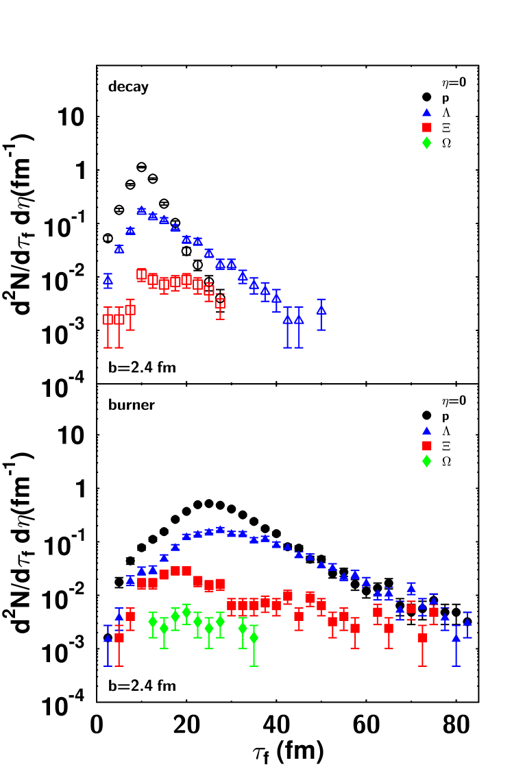
Figure 22: The freezeout time distribution of baryons for hydro+decay (open symbols, above) and hydro + UrQMD (solid symbols, below) at mid rapidity.

Figure 23 shows collision rates for meson-meson, meson-baryon and baryon-baryon collisions at mid-rapidity and an impact parameter of $b=2.4$ fm. We find that the reaction dynamics in the hadronic phase is dominated by meson-meson and to a lesser degree by meson-baryon interactions. Baryons essentially propagate in a medium dominated by mesons – a situation very different from the regime at AGS and lower SPS energies.

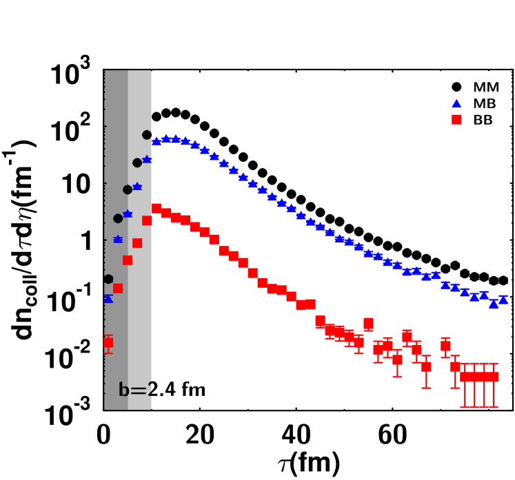
Figure 23: Collision rate for meson-meson (MM), meson-baryon (MB) and baryon-baryon (BB) at central collisions. The (dark) grey zone stands for qgp (mixed) phase, which is determined by the center cell.

Finally, let us move to the analysis of elliptic flow in the hydro+micro approach: First we show the elliptic flow coefficient $v_{2}$ as a function of $P_{T}$ for $\pi^{+}$ at centralities 5-10 % and 10-20 % in Fig. 24. Open symbols stand for experimental data and solid symbols represent our calculations. We find that the hydro+micro approach is able to provide an improved agreement to the data compared to the purely hydrodynamic calculation (see Fig. 24 for comparison).

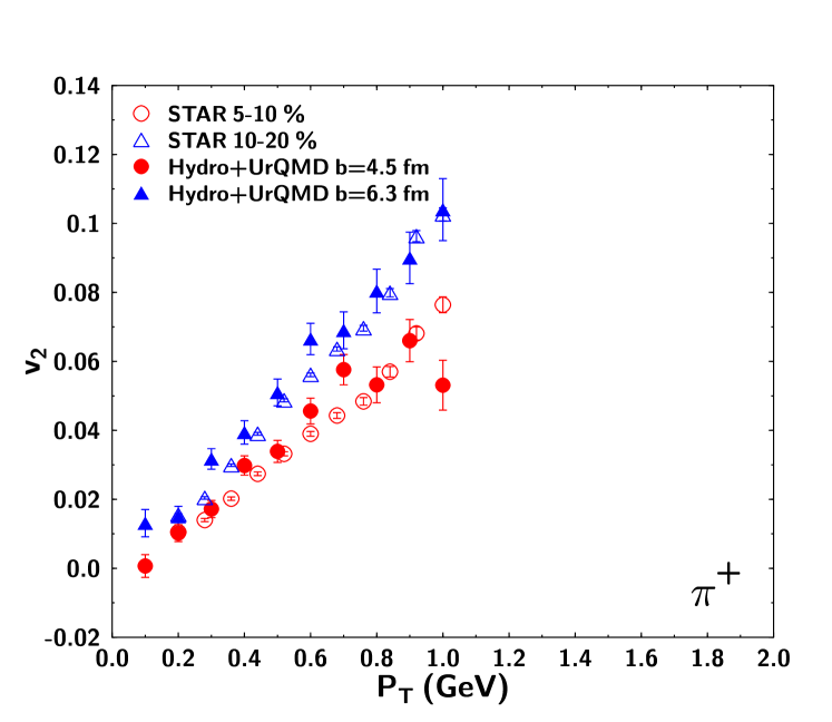
Figure 24: Elliptic flow as a function of $P_{T}$ for $\pi^{+}$ at centralities 5-10 % and 10-20 %. Open symbols stand for STAR data and solid symbols stands for our results.

Figure 25 shows the elliptic flow coefficient $v_{2}$ as a function of pseudo-rapidity $\eta$ for charged particles in central (3-15 %) (a) and mid central (15-25 %) (b) collisions. The solid line stands for a purely hydrodynamic calculation whereas the solid circles denote the hydro+micro approach and the solid triangles represent PHOBOS data PHOBOS_v2_eta . We find that the dissipative effects contained in the hydro+micro approach significantly alter the shape of the $v_{2}$ vs. $\eta$ curve, providing a far better agreement to the data – in particular for pseudo-rapidities away from mid-rapidity. The analysis shows that apparently dissipative effects increase towards projectile and target rapidities, where the assumptions of ideal fluid dynamics break down earlier. Our analysis confirms the findings of Hirano:2005xf , who in addition also studied the effect of a Color-Glass initial condition on the elliptic flow rapidity dependence.

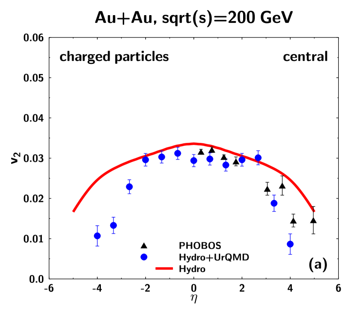
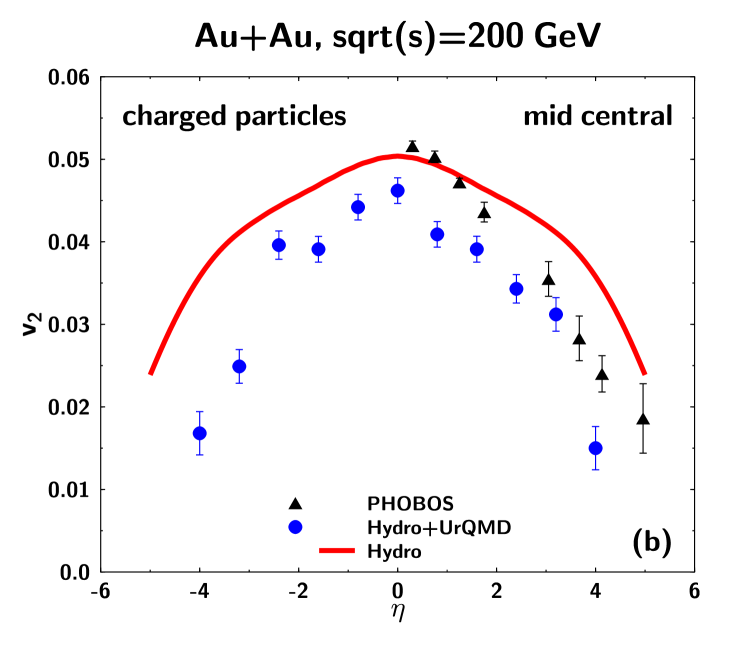
Figure 25: Elliptic flow as a function of $\eta$ of charged particles at central collisions (a) and mid central collisions (b). Impact parameters in the calculation are set to 4.5 fm (a) and 6.3 fm (b), respectively. The solid line stands for the 3-D pure hydrodynamic calculation and solid circles stand for results by hydro+UrQMD with PHOBOS data PHOBOS_v2_eta .

The question of how much elliptic flow develops during the deconfined phase vs. the hadronic phase is investigated in Figs. 26 and 27. It has been pointed out repeatedly, both in the framework of microscopic Sorge:1996pc as well as as hydrodynamic analysis KoSoHe00 that elliptic flow develops early on during the deconfined phase of the reaction and thus serves as a sensitive tool to the equation of state of QCD matter. This picture has been confirmed by the experimentally observed quark number scaling $v^{h}_{2}\sim nv_{2}(1/nP_{T})$ of elliptic flow at intermediate transverse momenta $P_{T}$ Adams:2003am ; Molnar:2003ff .

In Fig. 26 we plot elliptic flow $v_{2}$ as a function of $P_{T}$. The solid line stands for the pure hydro calculation, terminated at the switching temperature $T_{\rm sw}$ and solid circles denote the full hydro+micro calculation. We find that the QGP contribution to the elliptic flow depends on the transverse momentum – for low $P_{T}$ nearly 100% of the elliptic flow is created in the QGP phase of the reaction, whereas the hadronic phase contribution increases to 25% at a $P_{T}$ of 1 GeV/c.

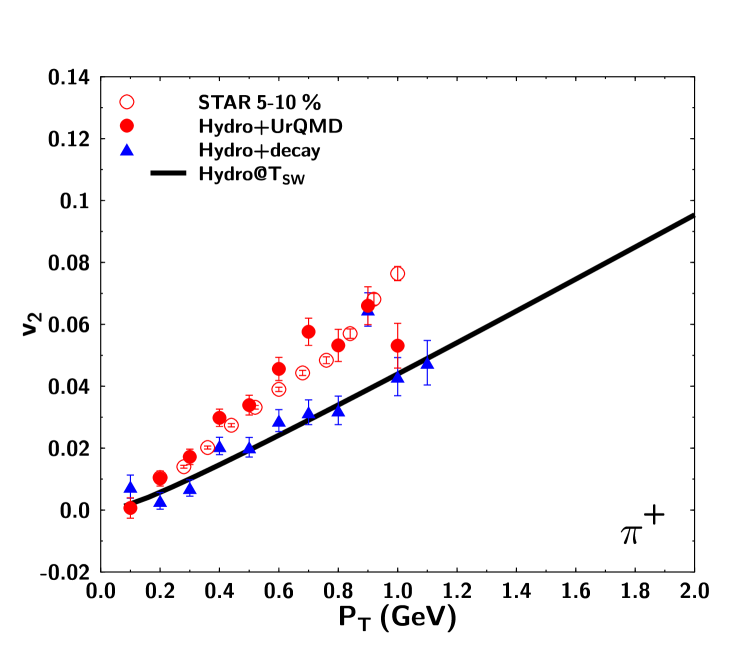
Figure 26: Elliptic flow as a function of $P_{T}$ of $\pi^{+}$ at centrality 5-10 % from pure hydro at the switching temperature (solid line), hydro + decay (solid triangles) and hydro + UrQMD (solid circles). Open symbols stand for experimental data from STAR.

Figure 27 shows the elliptic flow as a function of $\eta$: the pure hydrodynamic calculation is shown by the solid curve, the hydrodynamic contribution at $T_{\rm sw}$ is denoted by the dashed line and the full hydro+micro calculation is given by the solid circles, together with PHOBOS data (solid triangles). The shape of the elliptic flow in the pure hydrodynamic calculation at $T_{\rm sw}$ is quite different from that of the full hydrodynamic one terminated at a freeze-out temperature of 110 MeV. Apparently the slight bump at forward and backward rapidities observed in the full hydrodynamic calculation develops first in the later hadronic phase, since it is not observed in the calculation terminated at $T_{\rm sw}$. Evolving the hadronic phase in the hydro+micro approach will increase the elliptic flow at central rapidities, but not in the projectile and target rapidity domains. As a result, the elliptic flow calculation in the hydro+micro approach is closer to the experimental data when compared to the pure hydrodynamic calculation.

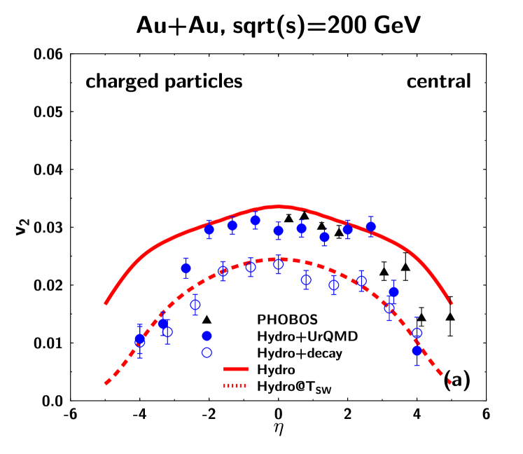
Figure 27: Elliptic flow as a function of $\eta$ of charged particles. Solid line and dashed lines stand for pure hydro calculation at the freezeout temperature (110 MeV) and the switching temperature, respectively. Experimental data by PHOBOS is shown with solid triangles. Open (Solid) circles stand for hydro + decay (hydro + UrQMD).

IV Summary and outlook

In summary, we have introduced a hybrid macroscopic/microscopic transport approach, combining a newly developed relativistic 3+1 dimensional hydrodynamic model for the early deconfined stage of the reaction and the hadronization process with a microscopic non-equilibrium model for the later hadronic stage at which the hydrodynamic equilibrium assumptions are not valid anymore. Within this approach we have dynamically calculated the freezeout of the hadronic system, accounting for the collective flow on the hadronization hypersurface generated by the QGP expansion. We have compared the results of our hybrid model and of a calculation utilizing our hydrodynamic model for the full evolution of the reaction to experimental data. This comparison has allowed us to quantify the strength of dissipative effects prevalent in the later hadronic phase of the reaction, which cannot be properly treated in the framework of ideal hydrodynamics.

Overall, the improved treatment of the hadronic phase provides a far better agreement between transport calculation and data, in particular concerning the flavor dependence of radial flow observables and the collective behavior of matter at forward/backward rapidities. We find that the hadronic phase of the heavy-ion reaction at top RHIC energy is of significant duration (at least 10 fm/c) and that hadronic freeze-out is a continuous process, strongly depending on hadron flavor and momenta.

With this work we have established a base-line – both for the regular 3+1 dimensional hydrodynamic model as well as for the hybrid hydro+micro approach. In forthcoming publications we shall expand on this baseline by investigating the effects of a realistic lattice-QCD motivated equation of state containing a tri-critical point and by performing an analysis of two particle correlations (HBT interferometry). We also plan to use our model as the medium for the propagation of jets and heavy quarks and to study the modification of our medium due to the passage of these hard probes.

V appendix

Equation (1) in $(\tau,x,y,\eta)$ is written in the following explicit way,

$$\left(\begin{array}[]{ccccc}\tilde{\gamma}^{2}\tilde{v}_{x}&\tilde{\gamma}^{2}\tilde{v}_{y}&\tilde{\gamma}^{2}\tilde{v}_{\eta}&\frac{1}{\omega}\frac{d\epsilon}{dT}&\frac{1}{\omega}\frac{d\epsilon}{d\mu}\\ \tilde{\gamma}^{2}&0&0&\frac{1}{\omega}\tilde{v}_{x}\frac{dp}{dT}&\frac{1}{\omega}\tilde{v}_{x}\frac{dp}{d\mu}\\ 0&\tilde{\gamma}^{2}&0&\frac{1}{\omega}\tilde{v}_{y}\frac{dp}{dT}&\frac{1}{\omega}\tilde{v}_{y}\frac{dp}{d\mu}\\ 0&0&\tilde{\gamma}^{2}&\frac{1}{\omega}\tilde{v}_{\eta}\frac{dp}{dT}&\frac{1}{\omega}\tilde{v}_{\eta}\frac{dp}{d\mu}\\ n_{B}\tilde{\gamma}^{2}\tilde{v}_{x}&n_{B}\tilde{\gamma}^{2}\tilde{v}_{y}&n_{B}\tilde{\gamma}^{2}\tilde{v}_{y}&\frac{dn_{B}}{dT}&\frac{dn_{B}}{d\mu}\\ \end{array}\right)\partial_{\tau}\left(\begin{array}[]{c}\tilde{v}_{x}\\ \tilde{v}_{y}\\ \tilde{v}_{\eta}\\ T\\ \mu\end{array}\right)$$ (42)

$$+ \left(\begin{array}[]{ccccc}\tilde{\gamma}^{2}\tilde{v}_{x}^{2}+1&\tilde{\gamma}^{2}\tilde{v}_{x}\tilde{v}_{y}&\tilde{\gamma}^{2}\tilde{v}_{x}\tilde{v}_{\eta}&\frac{1}{\omega}\tilde{v}_{x}\frac{d\epsilon}{dT}&\frac{1}{\omega}\tilde{v}_{x}\frac{d\epsilon}{d\mu}\\ \tilde{\gamma}^{2}\tilde{v}_{x}&0&0&\frac{1}{\omega}\frac{dp}{dT}&\frac{1}{\omega}\frac{dp}{d\mu}\\ 0&\tilde{\gamma}^{2}\tilde{v}_{x}&0&0&0\\ 0&0&\tilde{\gamma}^{2}\tilde{v}_{x}&0&0\\ n_{B}(\tilde{\gamma}^{2}\tilde{v}_{x}^{2}+1)&n_{B}\tilde{\gamma}^{2}\tilde{v}_{x}\tilde{v}_{y}&n_{B}\tilde{\gamma}^{2}\tilde{v}_{x}\tilde{v}_{\eta}&\tilde{v}_{x}\frac{dn_{B}}{dT}&\tilde{v}_{x}\frac{dn_{B}}{d\mu}\\ \end{array}\right)\partial_{x}\left(\begin{array}[]{c}\tilde{v}_{x}\\ \tilde{v}_{y}\\ \tilde{v}_{\eta}\\ T\\ \mu\end{array}\right)$$ (53)

$$+ \left(\begin{array}[]{ccccc}\tilde{\gamma}^{2}\tilde{v}_{y}\tilde{v}_{x}&\tilde{\gamma}^{2}\tilde{v}_{y}^{2}+1&\tilde{\gamma}^{2}\tilde{v}_{y}\tilde{v}_{\eta}&\frac{1}{\omega}\tilde{v}_{y}\frac{d\epsilon}{dT}&\frac{1}{\omega}\tilde{v}_{y}\frac{d\epsilon}{d\mu}\\ \tilde{\gamma}^{2}\tilde{v}_{y}&0&0&0&0\\ 0&\tilde{\gamma}^{2}\tilde{v}_{y}&0&\frac{1}{\omega}\frac{dp}{dT}&\frac{1}{\omega}\frac{dp}{d\mu}\\ 0&0&\tilde{\gamma}^{2}\tilde{v}_{y}&0&0\\ n_{B}\tilde{\gamma}^{2}\tilde{v}_{x}\tilde{v}_{y}&n_{B}(\tilde{\gamma}^{2}\tilde{v}_{y}^{2}+1)&n_{B}\tilde{\gamma}^{2}\tilde{v}_{y}\tilde{v}_{\eta}&\tilde{v}_{y}\frac{dn_{B}}{dT}&\tilde{v}_{y}\frac{dn_{B}}{d\mu}\end{array}\right)\partial_{y}\left(\begin{array}[]{c}\tilde{v}_{x}\\ \tilde{v}_{y}\\ \tilde{v}_{\eta}\\ T\\ \mu\end{array}\right)$$ (64)

$$+ \left(\begin{array}[]{ccccc}\tilde{\gamma}^{2}\tilde{v}_{\eta}\tilde{v}_{x}&\tilde{\gamma}^{2}\tilde{v}_{\eta}\tilde{v}_{y}&\tilde{\gamma}^{2}\tilde{v}_{\eta}^{2}+1&\frac{1}{\omega}\tilde{v}_{\eta}\frac{d\epsilon}{dT}&\frac{1}{\omega}\tilde{v}_{\eta}\frac{d\epsilon}{d\mu}\\ \tilde{\gamma}^{2}\tilde{v}_{\eta}&0&0&0&0\\ 0&\tilde{\gamma}^{2}\tilde{v}_{\eta}&0&0&0\\ 0&0&\tilde{\gamma}^{2}\tilde{v}_{\eta}&\frac{1}{\omega}\frac{dp}{dT}&\frac{1}{\omega}\frac{dp}{d\mu}\\ n_{B}\tilde{\gamma}^{2}\tilde{v}_{x}\tilde{v}_{\eta}&n_{B}\tilde{\gamma}^{2}\tilde{v}_{\eta}\tilde{v}_{y}&n_{B}(\tilde{\gamma}^{2}\tilde{v}_{\eta}^{2}+1)&\tilde{v}_{\eta}\frac{dn_{B}}{dT}&\tilde{v}_{\eta}\frac{dn_{B}}{d\mu}\end{array}\right)\frac{1}{\tau}\partial_{\eta}\left(\begin{array}[]{c}\tilde{v}_{x}\\ \tilde{v}_{y}\\ \tilde{v}_{\eta}\\ T\\ \mu\end{array}\right)$$ (75)

$$+ \left(\begin{array}[]{c}\frac{1}{\tau}\\ -\frac{1}{\tau}\tilde{v}_{x}\tilde{v}_{\eta}^{2}\tilde{\gamma}^{2}\\ -\frac{1}{\tau}\tilde{v}_{y}\tilde{v}_{\eta}^{2}\tilde{\gamma}^{2}\\ -\frac{1}{\tau}(\tilde{\gamma}^{2}\tilde{v}_{\eta}-\tilde{v}_{\eta}^{3}\tilde{\gamma}^{2})\\ \frac{1}{\tau}n_{B}\end{array}\right) =0,$$ (81)

where $\tilde{\gamma}=1/\sqrt{1-\tilde{v}_{x}^{2}-\tilde{v}_{y}^{2}-\tilde{v}_{\eta}^{2}}$, $Y_{L}=1/2\ln((1+v_{z})/(1-v_{z}))$. The difference between the relativistic hydrodynamic equations in Cartesian coordinates and those in the ($\tau,x,y,\eta$) coordinates is the addition of the fifth term in Eq. (81).

References

- (1) E.W. Kolb and M.S. Turner, “The Early Universe”, Frontiers in Physics 69 (Addison-Wesley, Redwood City, USA, 1990)
-
(2)
J.C. Collins and M.J. Perry, Phys. Rev. Lett. 34,
1353 (1975);
E.V. Shuryak, Phys. Rept. 61, 71 (1980);
K. Yagi, T. Hatsuda and Y. Miake, “Quark-Gluon Plasma”, (Cambridge Monographs on Particle Physics Nuclear Physics and Cosmology 23), Cambridge University Press, UK, 2005. -
(3)
B. B. Back et al. [PHOBOS Collaboration],
Phys. Rev. Lett. 85 (2000), 3100;
C. Adler et al. [STAR Collaboration], Phys. Rev. Lett. 86 (2001), 4778;
K. Adcox et al. [PHENIX Collaboration], Phys. Rev. Lett. 86 (2001), 3500;
K. Adcox et al. [PHENIX Collaboration], Phys. Rev. Lett. 87 (2001), 052301;
B. B. Back et al. [PHOBOS Collaboration], Phys. Rev. Lett. 87 (2001), 102301;
C. Adler et al. [STAR Collaboration], Phys. Rev. Lett. 87 (2001), 112303;
I. G. Bearden et al. [BRAHMS Collaboration], Phys. Rev. Lett. 87 (2001), 112305. -
(4)
K. H. Ackermann et al. [STAR Collaboration],
Phys. Rev. Lett. 86 (2001) 402;
C. Adler et al. [STAR Collaboration], Phys. Rev. Lett. 87 (2001), 182301. - (5) C. Adler et al. [STAR Collaboration], Phys. Rev. Lett. 87 (2001), 082301.
- (6) T. Ludlam, Nucl. Phys. A 750, 9 (2005).
- (7) M. Gyulassy and L. McLerran, Nucl. Phys. A 750, 30 (2005) [arXiv:nucl-th/0405013].
- (8) S.A. Bass, M. Gyulassy, H. Stöcker and W. Greiner, J. Phys. G25 (1999) R1.
- (9) J. D. Bjorken, Phys. Rev. D 27, 140 (1983).
- (10) R. B. Clare and D. Strottman, Phys. Rept. 141, 177 (1986).
- (11) A. Dumitru and D. H. Rischke, Phys. Rev. C 59, 354 (1999) [arXiv:nucl-th/9806003].
- (12) P. F. Kolb and U. W. Heinz, arXiv:nucl-th/0305084.
- (13) P. Huovinen, arXiv:nucl-th/0305064.
- (14) T. Hirano and K. Tsuda, Phys. Rev. C 66, 054905 (2002) [arXiv:nucl-th/0205043].
- (15) S. A. Bass and A. Dumitru, Phys. Rev. C61, 064909 (2000).
- (16) D. Teaney, J. Lauret, E. V. Shuryak, Phys. Rev. Lett. 86, 4783 (2003); ibid., nucl-th/011037.
- (17) T. Hirano, U. W. Heinz, D. Kharzeev, R. Lacey and Y. Nara, Phys. Lett. B 636, 299 (2006) [arXiv:nucl-th/0511046].
-
(18)
S. A. Bass, M. Belkacem, M. Bleicher, M. Brandstetter, L. Bravina,
C. Ernst, L. Gerland, M. Hofmann, S. Hofmann, J. Konopka, G. Mao,
L. Neise, S. Soff, C. Spieles, H. Weber, L. A. Winckelmann,
H. Stöcker, W. Greiner, C. Hartnack, J. Aichelin and N. Amelin,
Progr. Part. Nucl. Physics Vol. 41, 225 (1998),
nucl-th/9803035
M. Bleicher, E. Zabrodin, C. Spieles, S.A. Bass, C. Ernst, S. Soff, L. Bravina, M. Belkacem, H. Weber, H. Stöcker and W. Greiner, J. Phys. G25, 1859 (1999) - (19) C. Nonaka, E. Honda and S. Muroya, Eur. Phys. J. C17, 663 (2000).
- (20) T. Hirano, Phys. Rev. C65, 011901(R), (2001).
- (21) P. Huovinen, Nucl. Phys. A761, 296 (2005).
- (22) F. Karsch, J. Phys. G 31, S633 (2005) [arXiv:hep-lat/0412038].
- (23) C. Bernard et al. [MILC Collaboration], Phys. Rev. D 71, 034504 (2005) [arXiv:hep-lat/0405029].
- (24) M. G. Alford, K. Rajagopal and F. Wilczek, Phys. Lett. B 422, 247 (1998) [arXiv:hep-ph/9711395].
- (25) R. Rapp, T. Schafer, E. V. Shuryak and M. Velkovsky, Phys. Rev. Lett. 81, 53 (1998) [arXiv:hep-ph/9711396].
- (26) M. A. Stephanov, K. Rajagopal and E. V. Shuryak, Phys. Rev. Lett. 81, 4816 (1998) [arXiv:hep-ph/9806219].
- (27) Z. Fodor and S. D. Katz, JHEP 0203, 014 (2002) [arXiv:hep-lat/0106002].
- (28) R. Gavai, S. Gupta and R. Ray, Prog. Theor. Phys. Suppl. 153, 270 (2004) [arXiv:nucl-th/0312010].
- (29) C. R. Allton et al., Phys. Rev. D 66, 074507 (2002) [arXiv:hep-lat/0204010].
- (30) M. D’Elia and M. P. Lombardo, Phys. Rev. D 67, 014505 (2003) [arXiv:hep-lat/0209146].
- (31) Z. Fodor, S. D. Katz and K. K. Szabo, Phys. Lett. B 568, 73 (2003) [arXiv:hep-lat/0208078].
- (32) R. V. Gavai and S. Gupta, Phys. Rev. D 71, 114014 (2005) [arXiv:hep-lat/0412035].
- (33) Z. Fodor and S. D. Katz, JHEP 0404, 050 (2004) [arXiv:hep-lat/0402006].
- (34) S. Ejiri, C. R. Allton, S. J. Hands, O. Kaczmarek, F. Karsch, E. Laermann and C. Schmidt, Prog. Theor. Phys. Suppl. 153, 118 (2004) [arXiv:hep-lat/0312006].
- (35) J. Sollfrank, P. Huovinen, M. Kataja, P. V. Ruuskanen, M. Prakash, and R. Venugopalan, Phys. Rev. C55, 397 (1997).
- (36) C.M. Hung and E. Shuryak, Phys. Rev. C57, 1891 (1998)
- (37) D.H. Rischke, M.I. Gorenstein, H. Stöcker and W. Greiner, Z. Phys. C51 (1991).
-
(38)
U. Ornik, M. Plümer, B.R. Schlei, D. Strottman, and R.M. Weiner,
Phys. Rev. C54, 1381 (1996);
B.R. Schlei, U. Ornik, M. Plümer, D. Strottman, and R.M. Weiner, Phys. Lett. B376, 212 (1996);
B.R. Schlei, Heavy Ion Phys. 5, 403 (1997);
N. Arbex, U. Ornik, M. Plümer, and R.M. Weiner, Phys. Rev. C55, 860 (1997). - (39) J. Sollfrank, P. Huovinen, P. V. Ruuskanen, Eur. Phys. J C6, 525 (1999); ibid., nucl-th/9706012.
- (40) A. Dumitru and D. H. Rischke, Phys. Rev. C 59, 354 (1999) [arXiv:nucl-th/9806003].
- (41) A. Dumitru, C. Spieles, H. Stöcker, and C. Greiner, Phys. Rev. C56, 2202 (1997).
- (42) J. Cleymans, K. Redlich, and D.K. Srivastava, Phys. Rev. C55, 1431 (1997).
- (43) M. Belkacem, M. Brandstetter, S.A. Bass, M. Bleicher, L.V. Bravina, M.I. Gorenstein, J. Konopka, L. Neise, C. Spieles, S. Soff, H. Weber, H. Stöcker and W. Greiner, Phys. Rev. C58, 1727 (1998).
- (44) C. Nonaka, M. Asakawa, Phys. Rev. C71, 044904 (2005).
- (45) Y. Hama, R.P.G. Andrade, F. Grassi, O. Socolowski Jr., T. Kodama, B. Tavares and S.S. Padula, hep-ph/0510096.
- (46) P. F. Kolb, U. Heinz, P. Huovinen, K. J. Eskola, K. Tuominen, Nucl. Phys. A696, 197 (2001).
- (47) T. Hirano and Y. Nara, Nucl. Phys. A743, 305 (2004).
- (48) T. Hirano, U. Heinz, D. Kharzeev, R. Loy and Y. Nara, nucl-th/0511046.
- (49) K. J. Eskola, H. Honkanen, H. Niemi, P. V. Ruuskanen and S. S. Räsänen, Phys. Rev. C72, 044904 (2005).
- (50) P. Huovinen, P. F. Kolb, U. Heinz, P. V. Ruuskanen, S. A. Voloshin, Phys. Lett. B503, 58 (2001).
- (51) T. Hirano and K. Tsuda, Phys. Rev. C66, 054905 (2002).
- (52) S. Mrowczynski, hep-ph/0511052.
- (53) P. Jacobs and G. Cooper, nucl-ex/0008015.
- (54) P. F. Kolb, J. Sollfrank and U. Heinz, Phys. Rev. C62, 054909 (2000).
- (55) U. Heinz, P. F. Kolb, Phys. Lett. B542, 216 (2002).
- (56) S. S. Adler (PHENIX Collaboration), Phys. Rev. Lett. 91, 072303 (2003).
- (57) P. F. Kolb and R. Rapp, Phys. Rev. C67, 044903 (2003).
- (58) Thorsten Renk, Phys. Rev. C70, 021903 (2004); hep-ph/0407164.
- (59) J-P. Blaizot, J-Y. Ollitrault, p. 393 Quark-Gluon Plasma (Advanced Series on Directions in High Energy Physics, Vol 6) by Rudolph C. Hwa (Editor),World Scientific Pub Co Inc (August 1, 1990).
- (60) F. Cooper and G. Frye, Phys. Rev. D10, 186 (1974).
- (61) D. Teaney, J. Lauret and E. V. Shuryak, arXiv:nucl-th/0110037.
-
(62)
Y. Yariv and Z. Fraenkel,
Phys. Rev. C20, 2227 (1979);
J. Cugnon, Phys. Rev. C22, 1885 (1980);
Y. Pang, T.J. Schlagel, and S.H. Kahana, Phys. Rev. Lett. 68, 2743 (1992). -
(63)
H. Kruse, B.V. Jacak, and H. Stöcker,
Phys. Rev. Lett. 54, 289 (1985);
J. Aichelin and G. Bertsch, Phys. Rev. C31, 1730 (1985);
J.J. Molitoris and H. Stöcker, Phys. Rev C32, R346 (1985);
K. Weber, B. Blattel, V. Koch, A. Lang, W. Cassing, and U. Mosel, Nucl. Phys. A515, 747 (1990);
B.A. Li and C. M. Ko, Phys. Rev. C52, 2037 (1995);
W. Ehehalt and W. Cassing, Nucl. Phys. A602, 449 (1996). -
(64)
J. Aichelin, A. Rosenhauer, G. Peilert, H. Stöcker, and W. Greiner,
Phys. Rev. Lett. 58, 1926 (1987);
G. Peilert, H. Stöcker, A. Rosenhauer, A. Bohnet, J. Aichelin, and W. Greiner, Phys. Rev. C39, 1402 (1989);
H. Sorge, H. Stöcker, and W. Greiner, Annals of Physics (N.Y.) 192, 266 (1989);
J. Aichelin, Phys. Rept. 202, 233 (1991). -
(65)
B. Andersson, G. Gustafson, G. Ingelman, and T. Sjöstrand,
Phys. Rept. 97, 31 (1983);
B. Andersson, G. Gustafson, and B. Nilsson-Almqvist, Nucl. Phys. B281, 289 (1987). -
(66)
F. Laue et al.,
Phys. Rev. Lett. 82, 1640 (1999);
W. Chang et al., nucl-ex/9904010. - (67) Particle-Data-Group, Phys. Rev. D54 (1996).
- (68) P. Danielewicz and G. F. Bertsch, Nucl. Phys. A533, 712 (1991).
- (69) S. S. Adler et al. (PHENIX Collaboration), Phys. Rev. C69, 034909 (2004).
- (70) U. Heinz and P. F. Kolb, hep-ph/0204061; P. Huovinen, Nucl. Phys. A715, 299c (2003).
- (71) D. Teaney, nucl-th/0204023.
- (72) K. Adcox et al. (PHENIX collaboration), Nucl. Phys. A757, 184 (2004).
- (73) B. B. Back et al. (PHOBOS Collaboration), Phys. Rev. Lett. 91, 052303 (2003).
- (74) T. Hirano, K. Morita, S. Muroya, C. Nonaka, Phys. ReV. C65, 061902 (2005), K. Morita, S. Muroya, C. Nonaka and T. Hirano, Phys. ReV. C 66, 054904 (2002).
- (75) J. Adams et al. (STAR Collaboration), Phys. Rev. C72, 014904 (2005).
- (76) B. B. Back et al. (PHOBOS Collaboration), Phys. Rev. C72, 051901(R) (2005).
- (77) R. Rapp and E. V. Shuryak, Phys. Rev. Lett. 86, 2980 (2001) [arXiv:hep-ph/0008326].
- (78) C. Greiner and S. Leupold, J. Phys. G 27, L95 (2001) [arXiv:nucl-th/0009036].
- (79) M. Estienne (for the STAR Collaboration), J. Phys. G31, S873 (2005).
- (80) J. Adames et al. (STAR Collaboration), Phys. Rev. Lett. 92, 182301 (2004).
- (81) H. van Hecke, H. Sorge and N. Xu, Phys. Rev. Lett. 81, 5764 (1998) [arXiv:nucl-th/9804035].
- (82) A. Dumitru, S. A. Bass, M. Bleicher, H. Stoecker and W. Greiner, Phys. Lett. B 460, 411 (1999) [arXiv:nucl-th/9901046].
-
(83)
P.G. Jones and the NA49 collaboration,
Nucl. Phys. A610, 188c (1996);
C. Bormann et al., (NA49 collaboration), J. Phys. G23, 1817 (1997);
H. Appelshäuser et al., (NA49 collaboration), Phys. Lett. B444, 523 (1998);
E. Andersen et al. (WA97 Collaboration), Phys. Lett. B433, 209 (1998);
E. Andersen et al. (WA97 Collaboration), J. Phys. G25, 181 (1999). - (84) H. Sorge, Phys. Rev. Lett. 78, 2309 (1997) [arXiv:nucl-th/9610026].
- (85) J. Adams et al. [STAR Collaboration], Phys. Rev. Lett. 92, 052302 (2004) [arXiv:nucl-ex/0306007].
- (86) D. Molnar and S. A. Voloshin, Phys. Rev. Lett. 91, 092301 (2003) [arXiv:nucl-th/0302014].