Flow Coefficients and Jet Characteristics in Heavy Ion Collisions

Abstract

Identifying jets in heavy ion collisions is of significant interest since the properties of jets are expected to get modified because of the formation of quark gluon plasma. The detection of jets is, however, difficult because of large number of non-jet hadrons produced in the collision process. In this work we propose a method of identifying a jet and determining its transverse momentum by means of flow analysis. This has been done an event-by-event basis.

Keywords: Fourier analysis, Relativistic heavy-ion collisions, collective flow, Jet properties and flow

I Introduction

Identification of jets in heavy ion collisions is an important and challenging problem for several reasons. First, the quenching of jets has been proposed as one of the signatures of the formation of quark gluon plasma (QGP) gyulassy1 ; gyulassy2 ; gyulassy3 . It is expected that when the leading parton, which eventually fragments into jet particles, passes through a medium consisting of QGP it would loose some or all of its energy, in a process which is analogous to the loss of energy of a fast charged particle in the electromagnetic plasma. The leading parton would also produce secondary quarks and gluons during the passage gyulassy4 , resulting in the change of the profile of the jet particles. Thus, the characteristics of jets produced in heavy ion collisions would be different from those produced in hadron-hadron or $e^{+}-e^{-}$ collisions. It has been argued that such a large modification of jets would not occur when the parton passes through hot hadronic gas. Jet quenching has already been observed by different experiments at RHIC phenixwp ; starwp . These studies are basically the correlation studies between the energetic hadrons which are expected to be the leading hadrons produced in a jet. However, it would be interesting to detect jets directly, as done in $e^{+}-e^{-}$ and hadron-hadron collisions or at least identify them in heavy ion collisions.

The jet properties, like the number of particles in a jet and the opening angle of the jet which are produced in elementary collisions, have been well investigated qcdjets1 ; qcdjets2 . Also there is a good theoretical understanding of these in terms of perturbative QCD and jet fragmentation functions qcdjets2 ; qcdjets3 . In case of nucleus-nucleus collisions, identification of the jets using the standard jet reconstruction algorithms such as cone or $k_{T}$ algorithms cone is extremely difficult, if not impossible, because of the large number of non-jet background particles produced during the collision of two heavy ions. It is true that the jet particles are produced in a narrow cone in $\eta$ ( the rapidity ) and $\phi$ ( the azimuthal angle ) and have large momenta. On the other hand the background particles are distributed over a large range of $\eta$ and spread more or less uniformly in $\phi$. Nevertheless there are large number of non-jet particles in the jet cone. This makes the removal of non-jet ( background ) particles from the jet cone and identification of the jet particles difficult. One may use momentum cutoff to filter out the bulk of the low momentum background particles. Even then, it turns out that there are always sufficiently large number of background particles in the jet cone for these algorithms to work.

Recently, we have developed a method for identification of jets in heavy ion collisions sahu04 . The method is based on the fact that the flow or Fourier coefficients for events containing jets have a typical structure ( see later for the details ) which allows one to identify the jet events, determine the jet opening angle and the associated number of particles in the jet. It was also shown that when there are two jets going back-to-back, the even flow coefficients are significantly larger than the odd ones, which helps in differentiating between the events having single jet and those having two jets with (almost) opposite momenta. In the present work we have further extended this method by computing transverse momentum weighted flow coefficients. Using these flow coefficients, we are able to estimate the transverse momentum ($p_{T}$) of the jet as well as the jet opening angle and the number of jet particles. We also find that when there are two back-to-back jets present in the data, the flow coefficients for even values of $m$ are larger and those for odd values of $m$ are close to zero. This is particularly useful because the behavior of the flow coefficients clearly differentiates between the events having back-to-back jets ( that is no jet quenching ) and the events having single jet, in which one of the fast parton is completely stopped.

We organize our work as follows: In Section 2, we briefly review the flow method of characterizing jets and derive the results when the transverse momentum weighted flow coefficients are computed. We then discuss how these results, along with the results of the previous work sahu04 can be used to determine the properties of the jet which is followed by the analysis of the simulated data using our method and determination of the jet characteristics in Section 3. Section 4 concludes this study.

II Jet Identification From Flow Coefficients

The flow coefficients are nothing but the Fourier coefficients of the azimuthal distribution of particles produced in heavy ion collisions. These are determined by doing Fourier analysis of the collisions data. Thus, given a normalized distribution of particles, $P(\phi)$ in azimuthal angle, we can expand it in Fourier series voloshin

$$P(\phi)=\frac{1}{2\pi}\sum_{m=0}^{\infty}2v_{m}\cos m(\phi-\phi_{m}).$$ (1)

The coefficients $v_{m}$’s are called flow coefficients and $\phi_{m}$ is $m$-dependent angle defn . Generally, one expects $\phi_{m}$ to coincide with the reaction plane from symmetry considerations. This is because the only preferred or special plane in a collision is the reaction plane defined by the collision axis and the impact parameter. The flow coefficients $v_{m}$ are then given by

$$v_{m}=\int_{0}^{2\pi}d\phi P(\phi)\cos m(\phi-\phi_{m}),$$ (2)

with $v_{0}=1$ because $P(\phi)$ is normalized. The computation of $v_{m}$ from eq(2) requires the knowledge of $\phi_{m}$. In the experiments, $\phi_{m}$ is not known a priori and there are inaccuracies in the determination of $\phi_{m}$ from the data. It is therefore convenient to eliminate $\phi_{m}$ and determine the flow coefficients by using two-particle correlation method bevelac ; bevelac1 ; ollitrault . One then has

$$v_{m}^{2}=\int d\phi_{1}d\phi_{2}P(\phi_{1})P(\phi_{2})\cos m(\phi_{1}-\phi_{2}).$$ (3)

In fact, it is advantageous to adopt the correlation method since it eliminates the errors present in the determination of $\phi_{m}$ and the errors arising from fluctuations due to finite number of detected particles. On the other hand, one of the disadvantages of the correlation method is that the sign of the flow coefficients is not determined. Our analysis, fortunately, does not depend on the sign of $v_{m}$’s. It is well known that the flow coefficients for $m=$1 and 2 give information about the early stages of the system evolution in heavy ion collisions starflow ; sorge ; na49flow . These $v_{1}$ and $v_{2}$ are well established for a wide range of energiessahu05 ; sahu02 ; sahu00 ; sahu98 . Recently, there have been some investigations on the physical interpretation of flow coefficient for larger values of $m$ ollitrault1 ; kolb ; lokhtin . However, in our opinion, this interpretation is not as appealing as the interpretation of $m=$1 and 2 in terms of asymmetry of collision and dynamical evolution of colliding nuclei. In passing we would like to note that the correlation method described above has been successfully applied for flow analysis of different heavy ion collision experiments starflow ; na49flow .

Our jet identification method is based on the fact that for particles distributed uniformly in $\phi$, ( $P(\phi)=1/2\pi$ ) all the flow coefficients ( except $v_{0}$ ) vanish. On the other hand, for a $\delta$ function distribution all $v_{m}$’s are unity. Thus if an event consists of a well-defined jet having a number of particles produced in a small cone in $\phi$ which is embedded in a uniform background, the flow coefficients would be abnormally large. In the following we shall quantify this statement by considering specific distribution functions for jet and background particles. At this stage, we would like to point out the difference between the usual calculations of flow coefficients, one is trying to deduce the nature of the collective dynamics which is represented by the bulk of the particle. In our calculation, on the other hand, we are interested in the effect of a set of particles having common features (In this case, these being emitted in a narrow cone in $\phi$) present in a large background, on the flow coefficients. The background particles may or may not have collective flow ( see later for the case in which the event has a jet in the presence of collective flow ).

The definition of the flow in eq(2) is not weighted by any physical quantity. One often defines flow of a physical quantity ( say transverse momentum ) by weighting the averages by the corresponding physical quantity voloshin . Thus, the transverse momentum flow $v_{m,p_{T}}$ is

$$v_{m,p_{T}}=\int_{0}^{2\pi}\int_{0}^{\infty}d\phi dp_{T}p_{T}P(\phi,p_{T})\cos m(\phi-\phi_{m}),$$ (4)

We may eliminate $\phi_{m}$ and determine the transverse momentum flow as

$$v_{m,p_{T}}^{2}=\int d\phi_{1}d\phi_{2}dp_{T1}dp_{T2}p_{T1}p_{T2}P(\phi_{1},p_{T1})P(\phi_{2},p_{T2})$$ (5)

$$\times\cos m(\phi_{1}-\phi_{2}).$$

For a given particle distribution in an experiment, the flow coefficients are determined by the following equations:

$$v_{m}^{2} = \frac{1}{N^{2}}\sum_{i,j}\cos m(\phi_{i}-\phi_{j})$$ (6)

$$\mathrm{and}$$

$$v_{m,p_{T}}^{2} = \frac{1}{N^{2}}\sum_{i,j}p_{T,i}p_{T,j}\cos m(\phi_{i}-\phi_{j}),$$ (7)

where $N$ is the number of particles in the event and $p_{T,i}$ is the transverse momentum of $i^{th}$ particle. Note the self-correlation ($i=j$ terms) is included in the expression above. Without self-correlation, $v_{m}^{2}$’s could be negative, which is unphysical.

In the following we shall embed one or two jets in the background particles in each event, then compute and study the behavior of the flow coefficients. Considering a heavy ion collision event in which $N_{b}$ number of background particles in the event are distributed uniformly in azimuthal angle $\phi$ and their transverse momentum distribution is $f_{b}(p_{T})$. In addition there are $N_{j}$ number of jet particles emitted in a jet cone of angle $\Delta\phi$ centered at $\phi_{0}$ and their transverse momentum distribution is $f(p_{T})$. We shall assume that the angular distribution is uniform between $\phi-\Delta\phi/2$ and $\phi+\Delta\phi/2$. Thus, the probability distribution of $N=N_{b}+N_{j}$ particles can be defined as

$$P(\phi,p_{T})=\frac{N_{b}}{N}P_{b}(\phi,p_{T})+\frac{N_{j}}{N}P_{j}(\phi,p_{T}),$$ (8)

where

$$P_{b}(\phi,p_{T}) = \frac{1}{2\pi}f_{b}(p_{T})\;\;\;\;\;{\mathrm{for}}\;\;0<\phi<2\pi$$

$$\mathrm{and}$$

$$P_{j}(\phi,p_{T}) = \frac{1}{\Delta\phi}f(p_{T}),\;\;\;\;\;{\mathrm{for}}\;\;\phi_{0}-\Delta\phi/2<\phi<\phi_{0}+\Delta\phi/2.$$

The transverse momentum distributions of background and jet particles have been normalized to unity. Thus $\int f(p_{T})dp_{T}=\int f_{b}(p_{T})dp_{T}=1$. For this distribution, the expression for flow coefficients $v_{m}$ is

$$v^{2}_{m} = \int d\phi_{1}d\phi_{2}dp_{T1}dp_{T2}P(\phi_{1},p_{T1})P(\phi_{2},p_{T2})\cos m(\phi_{1}-\phi_{2})$$ (9)

$$= \int d\phi_{1}d\phi_{2}dp_{T1}dp_{T2}P(\phi_{1},p_{T1})P(\phi_{2},p_{T2})$$

$$\times (\cos(m\phi_{1})\cos(m\phi_{2})+\sin(m\phi_{1})\sin(m\phi_{2}))$$

$$= \frac{N_{j}^{2}}{N^{2}}\Big{[}\int d\phi_{1}dp_{T1}P_{j}(\phi_{1},p_{T1})\cos m(\phi_{1}-\phi_{0})\Big{]}^{2}$$

$$= \frac{N_{j}^{2}}{N^{2}}\Big{[}j_{0}(m\Delta\phi/2)\Big{]}^{2}.$$

The last line in eq(9) follows from the fact that, by definition, the two-particle distribution function factorizes into a product of single particle distribution function and the jet distribution function is symmetric about $\phi_{0}$. Further, the background particles do not contribute since their distribution is independent of the azimuthal angle and all trigonometric integrals vanish. If we use the fact that the jet angle $\Delta\phi$ is small, we can expand the cosine function in powers of $\phi_{1}-\phi_{0}$, then we get

$$v^{2}_{m}=\frac{N_{j}^{2}}{N^{2}}\Big{[}1-\frac{m^{2}\Delta\phi^{2}}{12}+{\cal O}(m^{4})\Big{]}.$$ (10)

The results in eq (10) has been obtained for a specific azimuthal distribution of jet particles. For this distribution, the variance $\sigma=\sqrt{(\phi^{2}_{av})-(\phi_{av})^{2}}=\frac{\Delta\phi}{\sqrt{12}}$. In fact, for general azimuthal distribution function, we can show that sahu04

$$v^{2}_{m}=\frac{N_{j}^{2}}{N^{2}}\Big{[}1-m^{2}\sigma^{2}+{\cal O}(m^{4})\Big{]},$$ (11)

where we assume that the jet particles are distributed according to a probability distribution function which is symmetric about $\phi_{0}$. One important point to notice in the expression above is that the flow coefficients don’t depend on the distribution of the background particles, provided that these are distributed uniformly in azimuthal angle. Also, the details of transverse momentum dependence of the jet particles is integrated out.

Following the same methodology, the expression for $p_{T}$-weighted flow coefficients can be determined. One can write

$$v^{2}_{m,p_{T}} = \frac{N_{j}^{2}<p_{T}>^{2}}{N^{2}}\Big{[}j_{0}(m\Delta\phi/2)\Big{]}^{2}$$ (12)

$$= \frac{N_{j}^{2}<p_{T}>^{2}}{N^{2}}\Big{[}1-\frac{m^{2}\Delta\phi^{2}}{12}+{\cal O}(m^{4})\Big{]}$$

$$= \frac{N_{j}^{2}<p_{T}>^{2}}{N^{2}}\Big{[}1-m^{2}\sigma^{2}+{\cal O}(m^{4})\Big{]},$$

where $<p_{T}>=\int dp_{T}p_{T}f(p_{T})$ is the average transverse momentum carried by a particle in the jet. Thus $N_{j}<p_{T}>$ gives the total transverse momentum of the jet.

The expressions in eqs(10, 12) clearly suggest a method of obtaining jet properties from the flow coefficients. If one plots $v^{2}_{m}$ and $v^{2}_{m,p_{T}}$ vs $m^{2}$, the points would lie on a straight line. For $v^{2}_{m}$ vs $m^{2}$ the intercept of the line on y-axis will yield the number of jet particles and from $v^{2}_{m,p_{T}}$ vs $m^{2}$ plot the intercept on y-axis will give the transverse momentum of the jet ( since $N$, the total number of particles is known ). And from the slope, one can determine the opening angle ($\sigma$ or $\Delta\phi$). So, the procedure would be to fit a straight line to the computed flow coefficients and determine the intercept and the slope. These in turn would yield number of jet particles, jet transverse momentum and jet opening angle. Note that for linear fit the fitting procedure is trivial, with the slope, intercept and errors in these quantities being determined by algebraic expressions. It should be obvious that the analysis described above is necessarily event-by-event analysismorsch ; morsch1 .

We now come to the case when there are two jets. In particular, we shall consider two jets emitted at azimuthal angles $\phi$ and $\phi+\pi$. This is the case of interest because we expect that a hard parton scattering would produce such jets having equal and opposite jet momenta. We expect that quenching of one of the jets would broaden the other jet and/or produce more jet particles. Thus, the characteristics of the two back-to-back jets would be different. Further, in an extreme situation, the fast moving parton of one of the jets may be completely absorbed in the medium leading to removal of one of the jets. To consider such a situation, following particle distribution function $P(\phi,p_{T})$ is chosen.

$$P(\phi,p_{T})=\frac{N_{b}}{N}P_{b}(\phi,p_{T})+\frac{N_{j1}}{N}P_{j1}(\phi,p_{T})+\frac{N_{j2}}{N}P_{j2}(\phi,p_{T}),$$ (13)

where

$$P_{b}(\phi,p_{T}) = \frac{1}{2\pi}f_{b}(p_{T})\;\;\;\;\;{\mathrm{for}}\;\;0<\phi<2\pi$$ (14)

$$P_{j1}(\phi,p_{T}) = \frac{1}{\Delta\phi}f_{1}(p_{T})\;\;\;\;\;{\mathrm{for}}\;\;\phi_{0}-\Delta\phi_{1}/2<\phi<\phi_{0}+\Delta\phi_{1}/2$$ (15)

$$P_{j2}(\phi,p_{T}) = \frac{1}{\Delta\phi}f_{2}(p_{T})\;\;\;\;\;{\mathrm{for}}\;\;\phi_{0}-\Delta\phi_{2}/2<\phi+\pi<\phi_{0}+\Delta\phi_{2}/2.$$ (16)

Note that the number of jet particles, their opening angles and momentum distributions have been assumed to be different for the two jets. The computation of the flow coefficients can be carried out in the same fashion and the result is

$$v^{2}_{m} = \frac{1}{N^{2}}\Big{[}N_{j1}j_{0}(\frac{m\Delta\phi_{j1}}{2})$$

$$+ (-1)^{m}N_{j2}j_{0}(\frac{m\Delta\phi_{j2}}{2})\Big{]}^{2}$$

and

$$v^{2}_{m,p_{T}} = \frac{1}{N^{2}}\Big{[}<p_{T,1}>j_{0}(\frac{m\Delta\phi_{j1}}{2})$$ (19)

$$+(-1)^{m}<p_{T,2}>j_{0}(\frac{m\Delta\phi_{j2}}{2})\Big{]}^{2}.$$

The result can be understood as follows. As in the case of a single jet, the background particles being uniformly distributed in azimuthal angle, which do not contribute to the flow coefficients. But, for two-jet case, there is nonzero contribution from the two particles in the same jet as well as the two particles belonging to different jets. The former corresponds to the square of the individual terms in the brackets of expressions above. The latter corresponds to the crossed terms. The factor of $(-1)^{m}$ in the expression above arises because the jet angles of the two jets differ by $\pi$. As in the case of a single jet, we may expand the Bessel function $j_{0}$ in the powers of its argument. However this does not yield a simple enough formula which can be used for determining the properties of the two jets. Further more, since only a few values of flow coefficients can be determined reliably, the determination of the properties of both of the jets ( i.e. the number of particles in each jet and the opening angles ) from the flow coefficients cannot be done reliably. Nevertheless, we can deduce some qualitative conclusions from these expressions. First, for two jet case, the flow coefficients for even $m$ are significantly larger than those for odd $m$. Particularly, if the two jets have similar opening angles and numbers of jet particles, the odd flow coefficients are expected to be close to zero and much smaller than the even coefficients. On the other hand, if the opening angle of one of the jets is broadened significantly, the corresponding Bessel function would decrease rapidly with $m$ and the pattern would look more like a single jet case. In reality, one may not get back-to-back jets even in hadron-hadron collision. This is due to the fact that the partons have internal motion within a hadron and sometimes a scattered parton may emit another hard parton, thus producing a more than two-jet like structure. In that case, the angle between two jets would not be $180^{o}$ but close to it and hence, the odd flow coefficients will not vanish but would still be small. We will discuss this in the next section, when there will be two jets with background particles.

III Determination of Jet Properties

In the preceding section we have shown that the flow coefficients have a characteristically different structure when there are jets present in the event. In particular, we have shown that, for small enough jet opening angle ( $\Delta\phi$ ), the square of the flow coefficients, $v^{2}_{m}$, have linear dependence on $m^{2}$. Further, we have shown that the intercept and slope of a linear fit gives the information about the number of particles in the jet, jet opening angle and the transverse momentum of the jet. In this section we shall apply this method and describe the results of such a program. The calculation is performed as follows. For an event with $N$ particles, we compute the flow coefficients $v^{2}_{m}=\frac{\sum_{i,j}\cos(m(\phi_{i}-\phi_{j}))}{N^{2}}$. Fitting a curve $b-cm^{2}$ to these values by minimizing $\chi^{2}$, we obtain the number of jet particles ( $N_{j}^{2}=bN^{2}$ ) and the jet opening angle ( $\Delta\phi^{2}=12cN^{2}/N_{j}^{2}=12c/b$ ). The fitting procedure also gives the error in $N_{j}$ and $\Delta\phi$. A similar calculation for $p_{T}$-weighted flow coefficients gives transverse momentum of the jet ( $N_{j}<p_{T}>$ ) as well as $\Delta\phi$.

Before going on to the discussion of the results, let us first consider the possible limitations of the method. One situation where the method would fail is when the number of background particles is large. This is because the expressions of the flow coefficients ( eqs(10, 12 ) ) have $N^{2}$ in the denominator. So, when the number of background particles is much larger than the number of jet particles, the flow coefficients would be numerically small. In that case, there would be a large error in the determination of the intercept as well as the slope from the flow coefficients. In fact, we can estimate the limit an the number of background particle, above which the method would fail. Given that there are $N_{b}$ background particles uniformly distributed in azimuthal angle, the average number of background particles in the jet cone is $N_{c}=\Delta\phi N_{b}/(2\pi)$. However, the background particles are distributed statistically and the fluctuations in the background particles in the jet cone is of the order of $\sqrt{N_{c}}$. Thus the method would work so long as $\sqrt{N_{c}}$ is smaller than the number of jet particles. This problem can be considerably reduced by removing small transverse momentum particles (which are predominantly non-jet particles) from the analysis. The method would also fail when $\Delta\phi$ is large. This is because, in this case, the power series expansion of the Bessel function in eqs(10, 12) is valid for few values of $m$. Roughly speaking, $m\Delta\phi/\sqrt{12}$ should be less than 1 for the series expansion of the Bessel function to work. This means that for typical jet opening angle of 0.5 radians, $m$ should be restricted to 6 or less. For larger $\Delta\phi$, $m$ is reduced further. Finally, we note that $N$ cannot be too small either because for very small $N$, there are large statistical fluctuations in the distribution of the background particles. This gives rise to large spurious flow coefficients from the background particles, thus affecting the fitting procedure.

One may think that when the events have dynamical flow, such as elliptical flow, this flow of the background particles will interfere with the flow coefficients arising from the jet particles. Fortunately, this is not the case because the values of the elliptic flow due to dynamics are not very large. Typically, the dynamical elliptical flow is observed to be of the order of $10-15\%$. Since we are determining $v_{m}^{2}$, the contribution of dynamical elliptic flow to $v_{2}^{2}$ is $\sim 0.01-0.02$. We shall see later that in the presence of a jet, $v_{m}^{2}$’s are $\sim 0.1$. Thus, the contribution of the dynamical flow much smaller than that due to a jet and therefore the dynamical flow does not affect the determination of jet properties very much.

To test the method we first generate events in which the background particles are produced from HIJING event generator hijing by switching off the jet production. The collision energy is 5.5 TeV/nucleon in center of mass for $Pb+Pb$ collision. This corresponds to the energy at LHC. Total of 3000 such events with impact parameter between 3 and 7 fm have been generated. Charged particles within one unit of rapidity at mid-rapidity are considered for the analysis. We have then added a single jet at a randomly chosen jet angle $\phi_{0}$ with $N_{j}$ number of jet particles. The jet particles are assumed to be distributed uniformly within a jet cone angle of $\Delta\phi$. The normalized $p_{T}$-distribution function $f(p_{T})=\alpha e^{-\alpha(p_{T}-\beta)}$ with $p_{T}$ between $\beta$ and $\infty$ and $\alpha=1.2$ GeV^-1 and $\beta=1$ GeV. Thus $\int dp_{T}P(p_{T})=1$ and $<p_{T}>=\int dp_{T}p_{T}P(p_{T})=\beta+1/\alpha=1.83$ GeV. The analysis is done for the number of jet particles varying from 10 to 20, the opening angle between $\pi/6$ and $\pi/4$ radians. The analyses are done by using a $p_{T}$ cut of 0.5, 0.75 and 1 GeV for background particles. The results are discussed below.

Further, we have also tested our method using HIJING event generator with default jet production in all events in the $Pb-Pb$ collision at 5.5 $TeV$/nucleon and between impact parameters 3 to 7 fm. This is done to check if our method can detect events having one and two jets successfully. Computations are done for $p_{T}=0.75$ GeV cuts and with and without $p_{T}$ weights. It may be noted that jet events with large energy and large number of jet particles are rare. So, not every event has dominant jet-like structure.

III.1 Only background particles

The case of only background particles is essentially considered to set the scale. The background particles are generated from HIJING event generators with the option of switching off the jet production and the hard processes. Therefore, the background particles in HIJING event generators are only due to the emission of soft particles and no high $p_{T}$ particles. Here we do not expect any structure in the flow coefficients as no jet is present in the data. Ideally, the flow coefficients should vanish since the particles are distributed uniformly in azimuthal angle. However, because of fluctuations associated with finite number of particles, we do obtain small nonzero values. In the limit of infinite number of background particles, $v_{m}^{2}$’s are expected to vanish. The flow coefficients for one such event without a jet are shown in Fig(1). In this figure the value of $p_{T}$ cut used is 0.75 GeV and the corresponding number of charged particles are around 60. One can see that the flow coefficients are indeed small and there is no systematic variation of these with $m$. Thus a meaningful linear fit cannot be obtained. The calculations also show that the flow coefficients systematically decrease as the transverse momentum cut is decreased ( thus increasing the number of background particles ). This behavior implies that the non-zero values of the flow coefficients are indeed due to fluctuations. We have analyzed 3000 such events and the behavior of the flow coefficients is qualitatively similar to that shown in Fig(1). The flow coefficients are generally smaller than 0.005 and 0.015 for constant weight and $p_{t}$ weighted coefficients respectively. We don’t find any event giving rise to flow coefficients which would mimic a jet. From this we conclude that these values of the flow coefficients set the scale for the background. For a meaningful analysis, the flow coefficients should be significantly larger than these values.

 

Figure 1: Plot of $v_{m}^{2}$ vs $m^{2}$ for the case of no jet. The closed (open) symbols are for with (without) $p_{T}$ weight.

III.2 Only Jet particles

We now consider the case when there are no background particles but only jet particles. This is like a jet produced in $e^{+}-e^{-}$ or hadron-hadron collision. The results obtained for this case are expected to agree very well with the input. We have put 10 jet particles within small angle($\Delta\phi$=$\pi$/6) per event. The flow coefficients $v_{m}^{2}$ vs $m^{2}$ has been shown in Fig(2) for both with and without $p_{T}$ weighted. The values of flow coefficients are large in comparison with the events having only background particles. The flow coefficients are nicely fitted with straight line. The intercept on the y-axis will give the number of jet particles and the transverse momentum of the jet. One such event is displayed in Fig(2).

 

Figure 2: Plot of $v_{m}^{2}$ vs $m^{2}$ for the case of only jet. The closed (open) symbols are for with (without) $p_{T}$ weight.

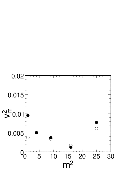
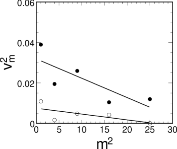
III.3 One Jet with Background

We shall now consider the case of one jet with background particles. A typical plot of $v_{m}^{2}$ vs $m^{2}$ for $p_{T}$ cut of 0.75 GeV for background particles and 10 jet particles is shown in the left panel of Fig(3). The plots for 0.5 and 1 GeV cuts are similar with $v_{m}^{2}$’s being smaller ( larger ) for 0.5 ( 1 ) GeV cut. We find that the flow coefficients are significantly larger than those obtained for an event without a jet, implying that the method is likely to work. Further, a reasonable linear fit to the data can be obtained. Both the with and without $p_{T}$-weighted flow coefficients are plotted in the left panel of Fig(3).

 

 

Figure 3: Plot for $v_{m}^{2}$ vs $m^{2}$ (left figure). The closed (open) symbols are for with (without) $p_{T}$ weight. The right figure shows the transverse momenta of the particles in a ’wagon-wheel’ plot. Each particle is represented by a line in the plot and the length and the direction give the transverse momentum and azimuthal angle of the particle.

Note that $v_{m}^{2}$ for $m=2$ is larger than 0.1. As mentioned earlier, $v_{2}^{2}$ for dynamical elliptic flow is expected to be 0.03 or less over a wide range of $p_{T}$ values starflow1 . Since the observed flow coefficient is order of magnitude larger than the expected dynamical flow value, we can definitely conclude that the analysis can be done even in the presence of non-zero elliptic flow. This is not to say that the dynamical collective flows cannot be determined by other means.

The right figure in Fig(3) shows the ’wagon-wheel’ plot of the same event. In this plot each line represents a particle in the event and the direction and the length of the line represents the azimuthal angle and the magnitude of transverse momentum of the particle respectively. One can clearly observe a cluster of particles in a small range of azimuthal angle near $\phi=7\pi/6$. These set of particles are responsible for the peculiar behavior of the flow coefficients seen in the left panel and these constitute a jet. In addition to this cluster, one can also observe few other clusters of fewer particles as well. These are essentially due to statistical fluctuations in the background. These fluctuations are responsible for the deviation from the expected linear behavior of the flow coefficients. However, one should note that in spite of these clusters, the linear pattern survives.

Table 1: The extracted values of number of jet particles, jet $p_{T}$ in GeV, opening angle in radians and error in these quantities. The errors are due to the error in obtaining slope and intercept from a linear fit to the square of the flow coefficients. The average over 3000 events is shown. The results for $p_{T}$ cuts of 0.5, 0.75 and 1.0 GeV are shown. The calculations are done for the jet opening angles of $\pi/6$ and $\pi/4$ radians. The computations are for 10 jet particles and jet $p_{T}$ of 18.26 GeV.

Input # of particles, jet $p_{T}$,	extracted values
$p_{T}$ cut and $\Delta\phi$	# of particles	jet $p_{T}$	$\Delta\phi$	$\Delta\phi$
			(with $p_{T}$ weight)	(without $p_{T}$ weight)
10, 18.26, 1.00, $\pi/6$	$10.52\pm 1.37$	$18.17\pm 1.75$	$0.43\pm 0.09$	$0.46\pm 0.08$
10, 18.26, 0.75, $\pi/6$	$11.60\pm 2.29$	$18.17\pm 2.47$	$0.46\pm 0.07$	$0.57\pm 0.008$
10, 18.26, 0.50, $\pi/6$	$14.11\pm 3.46$	$18.14\pm 3.11$	$0.56\pm 0.02$	$0.70\pm 0.10$
10, 18.26, 1.00, $\pi/4$	$10.31\pm 1.27$	$18.17\pm 1.65$	$0.54\pm 0.07$	$0.53\pm 0.08$
10, 18.26, 0.75, $\pi/4$	$11.44\pm 2.14$	$18.17\pm 2.31$	$0.53\pm 0.08$	$0.57\pm 0.04$
10, 18.26, 0.50, $\pi/4$	$14.05\pm 3.30$	$18.18\pm 2.85$	$0.54\pm 0.08$	$0.77\pm 0.16$
10, 18.26, 1.00, $\pi/8$	$10.56\pm 1.41$	$18.17\pm 1.80$	$0.39\pm 0.07$	$0.44\pm 0.06$
10, 18.26, 0.75, $\pi/8$	$11.63\pm 2.36$	$18.17\pm 2.55$	$0.45\pm 0.04$	$0.59\pm 0.03$
10, 18.26, 0.50, $\pi/8$	$14.23\pm 3.55$	$18.19\pm 3.18$	$0.51\pm 0.03$	$0.97\pm 0.37$

The results obtained after analyzing over 3000 events are summarized in Table - 1. The simulation is done for three different jet opening angles ( $\Delta\phi$ ) and three transverse momentum cuts are employed. The average of the extracted number of particles, jet transverse momentum and jet opening angle as well as the average estimated error is shown. Note that the error quoted is due to the uncertainty in the determination of the slope and intercept from $\chi^{2}$ fitting. Following conclusions can be drawn from these results.

• The extracted values of the opening angle $\Delta\phi$ are correlated with the corresponding input values. However, these are smaller for large opening angles. The errors in the extracted values are also large ( between 10 and 30 % ). The extracted opening angle values for without $p_{T}$-weight case are systematically higher for $p_{T}$ cut of 0.5 GeV. The agreement is better for smaller opening angles. The failure at the larger opening angle can be attributed to the failure of the expansion of the Bessel function in powers of $\Delta\phi^{2}m^{2}$ for larger $m$’s. One generally extracts larger slope and therefore larger opening angle if one uses fewer values of $m$ for fitting.

• For smaller $p_{T}$ cut the value of extracted opening angle is large and the error in it also equally large for without $p_{T}$ weighted values.

• Extracted values of number of jet particles agree better for larger $p_{T}$ cut. For the $p_{T}$ cut of 0.5 GeV the extracted number of jet particles is systematically larger by 40%. For 1 GeV cut, the agreement is very good. The error in the extracted values decreases almost linearly with $p_{T}$ cut.

• The extracted values of jet transverse momentum, on the other hand, agrees very well ( within 5% ) with the input value.

The reason for the $p_{T}$-weighted analysis working better than the constant weight can be understood as follows. Most of the background particles are having transverse momenta smaller than 1 GeV or so. Thus when one computes the $p_{T}$-weighted flow coefficients, the importance of the background particles in the flow coefficients is de-emphasized and large transverse momentum particles are given larger weight. Hence, to some extent, $p_{T}$ weighting plays the same role as that of transverse momentum cut. As a result the extracted $p_{T}$ of the jet does not appear to be sensitive to the transverse momentum cut applied in the analysis.

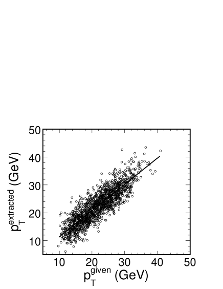
In our simulation of the jet event, the number of jet particles is fixed but the jet transverse momentum is not. This is because the transverse momentum of the jet particles is assigned statistically according to the transverse momentum distribution function $P(p_{T})$. Thus, although the jet transverse momentum is, on the average, given by the product of the average transverse momentum $<p_{T}>$ times the number of jet particles, the jet transverse momentum fluctuates, from event to event, about this number. This means that for a set of events with fixed number of jet particles, the jet transverse momentum is distributed over a range. If we consider the jets with different number of particles in a jet, we essentially generate a number of events with a broad distribution of jet transverse momenta. We can then look at the correlation between the input and extracted jet transverse momenta. Such a correlation between extracted and input jet transverse momentum is displayed in Fig(4). One can fit a nice straight line with the slope close to unity and the intercept close to zero, although the $\chi^{2}$ is rather large at 5.6.

 

Figure 4: Plot of extracted jet transverse momentum vs input transverse momentum. The graph shows a linear correlation between the two.

III.4 Two Jets with Background

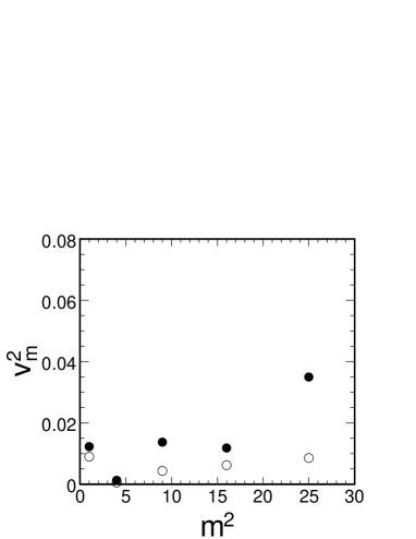
We have noted earlier that when we have two back-to-back jets, the flow coefficients show a distinct odd-even effect with the odd $v_{m}^{2}$’s being very small in comparison with those for even $m$. The suppression of the odd flow coefficients is maximum when the two jets have same opening angle and equal number of jet particles. We have also investigated the effect of varying the opening angle and number of particles of one of the jets. This, in some sense, is equivalent to partial quenching of one of the jets. The results of the investigation are shown in Fig (5). The closed symbols of left figure show the $v_{m}^{2}$ vs $m^{2}$ having different opening angle of both the jets. The open symbols are for both the jets having same opening angle.

 

 

Figure 5: Plot of $v_{m}^{2}$ vs $m^{2}$ (left figure). The closed (open) symbols are for with (without) $p_{T}$ weight for $p_{T}$ cut of 0.75 GeV. The figure on the right shows the transverse momenta of the particles in a ’wagon-wheel’ plot. Two back-to-back jets can be identified in the figure.

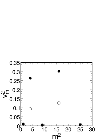
When the number of jet particles in one of the jets is reduced, the contribution of that jet to the flow coefficients decreases and naturally the plot starts looking like a single jet. The corresponding transverse momenta of the jet particles are shown in the ’wagon-wheel’ plot in Fig (5).

 

 

Figure 6: Plot of $v_{m}^{2}$ vs $m^{2}$ (left figure). The closed (open) symbols are for with (without) $p_{T}$ weight for $p_{T}=0.75$ GeV cut. The figure on the right shows the transverse momenta of the particles in a ’wagon-wheel’ plot. Two jets can be identified in the figure.

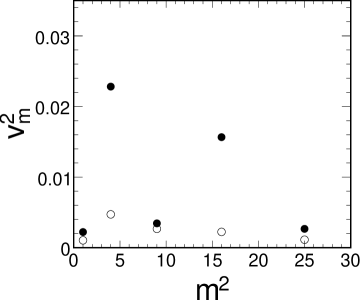
A few comments are in order at this stage. First, one does not really get back-to-back jets even in hadron-hadron collision because the partons have internal motion within a hadron and sometimes a scattered parton may emit another hard parton, thus producing a three-jet structure. In the first case, the angle between the two jets would not be $180^{o}$ but close to it. In that case, the odd flow coefficients will not vanish but would still be small. In the second case, we really do not have two jets so we should not expect to have the typical odd-even effect of two jets event. In case of nucleus-nucleus collision, one of the jets may be quenched or particles of one of the jets may scatter from the background. This would mean that the opening angle of this jet would be larger or there would be fewer particles in this jet. This means that as this effect becomes stronger, the structure of the event would go over from two jets event, with typical odd-even effect to single jet structure. In Fig(6), we have shown two jets event from HIJING event generators by switching on the jets. In this figure, the flow coefficient show a distinct odd-even structure in the plot of $v_{m}^{2}$ vs $m^{2}$, as we discussed above. In the next section we will discuss the events in HIJING by turning on the jet production in detail.

 

 

Figure 7: Plot of $v_{m}^{2}$ vs $m^{2}$ (left figure). The closed (open) symbols are for with (without) $p_{T}$ weight for $p_{T}=0.75$ GeV cut. The figure on the right shows the transverse momenta of the particles in a ’wagon-wheel’ plot. One jets can be identified in the figure. The extracted values of jet particles are $17.7\pm 4.4$, jet $p_{T}=29.6\pm 7.3$ GeV, $\Delta\phi=0.72\pm 0.34$( with $p_{T}$ weight) and $\Delta\phi=0.70\pm 0.32$ ( without $p_{T}$ weight).

 

 

Figure 8: Plot of $v_{m}^{2}$ vs $m^{2}$ (left figure). The closed (open) symbols are for with (without) $p_{T}$ weight for $p_{T}=0.75$ GeV cut. The figure on the right shows the transverse momenta of the particles in a ’wagon-wheel’ plot. This event shows no-jet by our method, though jets are present in this event, which is generated by HIJING.

III.5 HIJING Events with Jets

We now discuss the results for HIJING events with jets present. As mentioned earlier, high energy jets with large numbers of jet particles, which correspond to ( relatively ) hard collision of partons are rare. We are using HIJING parameters which allow maximum number of hard scatterings per nucleon-nucleon collision. It is not clear if this number is realistic but it does help in generating events having large energy jets having large number of jet particles. Of course most of the jets are mini-jets having few jet particles and our method is not expected to detect such mini-jets.

When an event has a single high energy jet with large number of particles ( and rest of the particles being produced by low energy jets and other background particles ), the flow coefficients are expected to have a typical behavior like those events considered above in Section 3.3 above. Further, when there are two almost back-to-back jets, the event would be similar to those discussed in Section 3.4 above. In other cases, the event is expected to look like the background only events discussed in Section 3.1 above. This is because, many low energy jets will have the azimuthal angle distribution of particles similar to that of background particles. Thus, by studying the flow coefficients we would be able to classify the HIJING events into three categories, namely, one jet events which have large flow coefficients, two jet events having oscillating flow coefficients and rest which have small flow coefficients which are almost random, not having any pattern.

We have analysed a few thousand HIJING events with jets switch on and we find that 50 to 60 % of the events can be classified as one or two jet events. The wagon-wheel plot as well as the plot of flow coefficients for one of the HIJING event identified as a single jet event is shown in Fig(7). Also similar plot for a typical event which has been classified as no-jet event by our method is displayed in Fig(8). There is a clear-cut correlation between the plot of flow coefficients ( which indicates whether the event would have jet structure or not ) and the wagon wheel plot ( which shows a jet on visual inspection ).

IV Conclusions

We have explored the possibility of identifying and characterizing the jet structure in a relativistic heavy ion collisions. The method exploits the fact that if the event has sufficiently large number of particles emitted in a narrow cone in azimuthal angle, the flow coefficients for such an event are abnormally large. Further, we have shown that in such a case, there is a linear relation between the square of the flow coefficients $v_{m}$ with $m^{2}$ and using this relation it is possible to estimate the number of jet particles, the jet opening angle and the jet transverse momentum. For the last quantity one has to compute the $p_{T}$ weighted flow coefficients. We have applied the method to simulated data having zero, one and two jets. We find that these three cases can be distinguished from the pattern of the flow coefficients. For the events with no jet, the flow coefficients are small. For one jet events, the flow coefficients are large and show the linear behavior discussed above. In case of the two jets, the odd and even flow coefficients fluctuate with the odd coefficients being small. We believe that from the observed behavior of the flow coefficients in an event, it would be possible to identify events in which one of the jet suffers quenching. We feel that this method can be used in LHC experiments to isolate collision events having one and two jets and possibly extract the properties of jets.

References

- (1) X.N.Wang and M.Gyulassy,Phys.Rev.Lett. 68 (1992) 1480.
- (2) M. Gyulassy, I. Vitev and X. -N. Wang, Phys. Rev. Lett. 86 (2001) 2537.
- (3) M. Gyulassy, Nucl. Phys. B571 (2000) 197.
- (4) M. Gyulassy, Nucl. Phys. A661 (1999) 637.
- (5) K. Adcox et al., [PHENIX Coll.], Nucl. Phys. A757 (2005) 184.
- (6) J. Adams et al. [STAR Coll.], Nucl. Phys. A757 (2005) 102.
- (7) B. Potter, Nucl. Phys. B540 (1999) 382.
- (8) R. K. Ellis, W. J. Stirling and B. R. Webber, QCD and Collider Physics (Cambridge University Press 1996).
- (9) X. N. Wang, Nucl. Phys. A702 (2002) 238.
- (10) G. C. Blazey et al., hep-ex/0005012.
- (11) S. C. Phatak and P. K. Sahu, Phys. Rev. C69 (2004) 024901.
- (12) A. M. Poskanzer and S. A. Voloshin, Phys. Rev. C58 (1998) 1671.
- (13) An alternate expansion is with and .
- (14) C. Pinkenberg et al. [E895 Collaboration], Phys. Rev. Lett. 83 (1999) 1295.
- (15) P. Danielewicz et al., Phys. Rev. C 38 (1998) 120.
- (16) N. Borghini, P. M. Dinh and J. -Y. Ollitrault, Phys. Rev. C64 (2001) 054901.
- (17) K. H. Ackermann et al. [STAR Collaboration], Phys. Rev. Lett. 86 (2001) 402.
- (18) H. Sorge, Phys. Rev. Lett. 82 (1999) 2048.
- (19) C. Alt et al. [NA49 Coll.], Phys. Rev. C68 (2003) 034903.
- (20) M. Isse, A. Ohnishi, N. Otuka, P. K. Sahu and Y. Nara, Phys. Rev. C72 (2005) 064908.
- (21) P. K. Sahu and W. Cassing, Nucl. Phys. A712 (2002) 357.
- (22) P. K. Sahu, W. Cassing, U. Mosel and A. Ohnishi, Nucl. Phys. A672 (2000) 376.
- (23) P. K. Sahu, A. Hombach, W. Cassing, M. Effenberger and U. Mosel, Nucl. Phys. A640 (1998) 493.
- (24) N. Borghini, P. M. Dinh and J. -Y. Ollitrault, Phys. Rev. C63 (2001) 054906.
- (25) P. F. Kolb, Phys. Rev. C68 (2003) 031902(R).
- (26) I. P. Lokhtin, L. I. Sarycheva, A. M. Snigirev, Eur. Phys. Journal C30 (2003) 103.
- (27) I.P. Lokhtin, L.I. Sarycheva, A.M. Snigirev, Physics Letters B537 (2002) 261.
- (28) A. Morsch (for the ALICE Collaboration), J. Phys. G31 (2005) S597.
- (29) Xin-Nian Wang and Miklos Gyulassy: Phys. Rev. D45 (1992) 844.
- (30) J. Adams et al. [STAR Collaboration], Phys. Rev. Lett. 92 (2001) 062301.