Transition from participant to spectator fragmentation in Au+Au reaction between 60 AMeV and 150 AMeV

Abstract

Using the quantum molecular dynamics approach, we analyze the results of the recent INDRA Au+Au experiments at GSI in the energy range between 60 AMeV and 150 AMeV. It turns out that in this energy region the transition toward a participant-spectator scenario takes place. The large Au+Au system displays in the simulations as in the experiment simultaneously dynamical and statistical behavior which we analyze in detail: The composition of fragments close to midrapidity follows statistical laws and the system shows bi-modality, i.e. a sudden transition between different fragmentation pattern as a function of the centrality as expected for a phase transition. The fragment spectra at small and large rapidities, on the other hand, are determined by dynamics and the system as a whole does not come to equilibrium, an observation which is confirmed by FOPI experiments for the same system.

I INTRODUCTION

Two decades after its discovery, the rich phenomenology of multifragmentation has been widely explored (for recent references see, e.g., indra1 ; indra2 ). It has been experimentally shown that in one single heavy ion collision many intermediate mass fragments (IMF’s) are produced, where IMF’s are defined as fragments with $3\leq Z\leq 25$. The upper limit is chosen to eliminate fission fragments. Nevertheless, some of the key questions are still not answered. One of these, perhaps the most central one in order to come to a better understanding, is the question how fragments are formed. There are two reasons for this. First of all, under the keyword multifragmentation two different processes are discussed which may be widely different in their physical origin. At low beam energies, the highest multiplicity of IMF’s is observed in central collisions. Fragments are formed from the matter in the geometrical overlap between projectile and target (participant matter). With increasing beam energy the multiplicity of IMF’s in central collisions decreases. At high beam energies, above several hundreds of AMeV, central collisions are that violent that only small nuclei, mainly up to mass $A=4$, survive and, therefore, the multiplicity of IMF’s is low. Here, the largest IMF multiplicity is found in semi-peripheral reactions, and the fragments originate from those nucleons which are NOT in the geometrical overlap zone of projectile and target, the so-called spectator matter. In this case, particles from the interaction zone penetrate into the spectator matter and cause its disintegration into IMF’s. The mean kinetic energy per nucleon of the fragments is lower than in central collisions at low beam energy alad . It is all but clear whether the two processes, the one forming fragments from hot (energy per particle well above the binding energy of fragment nucleons alad ) and dense matter and the other forming fragments from rather cold matter (energy per fragment below the binding energy alad ) and at around normal nuclear matter density, have the same physical origin.

Second, although completely different in their origin, statistical and dynamical models predict very similar results for several key observables. In the statistical or equilibrated source scenario fi ; bon95 ; ber ; QSM it is assumed that at a density which is a fraction of the normal nuclear matter density the interaction among the constituents suddenly stops (freezes out) and that the relative fragment abundances at that moment are given by the phase space at the freeze out volume. Thus this model assumes that at the latest at freeze out the system is in thermal or statistical equilibrium. The phase space is calculated either in a microcanonical or in a grand canonical approach. In either case, it is assumed that, at the end, the average thermal energy of the fragments is independent of the fragment size and, neglecting Coulomb interaction and an eventual collective flow, equals 3/2 $T$ in a grand-canonical formulation. For energies larger than 50 AMeV the mass yield of IMF’s follows a power law or an exponential function which can hardly be distinguished due to the small range of IMF masses.

The dynamical approach presented in ref.HI considers multifragmentation to be a fast process in which the nucleons do not have the time to come to equilibrium, similar to the shattering of glass. There the distribution of splinters follows also a power law although it is certainly not thermal. In the fragmentation process, the nucleons forming a fragment keep their momentum which they have initially due to Fermi motion. As shown by Goldhaber gol this fast fragmentation yields as well a mass independent average energy of the fragments of the order of 15 MeV and a spectrum similar to a thermal one. This means that single particle spectra cannot qualitatively distinguish between an already initially (due to the Fermi motion) present momentum distribution and a momentum distribution created by collisions in the expanding system. One can argue that the average energy should differ by a factor of two (the average energy of 15 MeV due to Fermi motion as compared to a maximal thermal energy (3/2 $T$) of 7.5 MeV because beyond a temperature of 5 MeV fragments are not stable anymore). If a transverse flow builds up during the expansion and in view of the additional Coulomb energy a distinction of the two slopes is only possible at high fragment kinetic energies. There the statistical error of the present experiments is too large for a distinction.

The scenario of a fast multifragmentation is also predicted by transport theories which describe the time evolution of the reaction starting from the initially separated projectile and target nuclei until the formation of the finally observed fragments. This models are either based on true n-body approaches har1 ; aic ; hartn ; reg ; AMD ; amdind or on the Boltzmann Uehling Uhlenbeck approach with fluctuating forcessur1 . In the former approach fragments are to a large extent initial correlations which have survived the heavy ion reaction. It is a challenge to understand why these initial-final state correlations produce seemingly the same results as the statistical models. The systems which have been investigated in these simulations so far are of moderate size. The recent Au+Au experiments of the INDRA collaboration at GSI in the beam energy range between 60 AMeV and 150 AMeV investigate really heavy systems (which may come closer to equilibrium than lighter systems) with one of the most advanced $4\pi$ detectors in the most interesting energy regime. In addition, the results can be compared with older experiments from the FOPI collaboration which cover a partially different phase space. Therefore it is possible to cross check the results and to control the filters. Putting both experiments together a very detailed picture of the interaction should emerge. This triggered a renewed effort to identify the origin of multifragmentation. For the experimental details of the INDRA experiment see ref. indra1 .

We start out in chapter two with an introduction to the Quantum Molecular Dynamics approach which we use to simulate the heavy ion reactions. Chapter 3 is devoted to the challenge to compare simulations with selected events. We will discuss in detail how the detector acceptance changes the 4$\pi$ particle distributions which are obtained in the simulation programs. There we discuss as well the importance to select the events in the same way as the experiments do. The much easier way to classify the theoretical simulation events according to the impact parameter picks events which can hardly be compared with an experimentally accessible event selection. In chapter 4 we discuss the global event structure and demonstrate that QMD produces well the experimental centrality classes. Chapters 5 and 6 are devoted to central collisions. Chapter 5 presents a comparison of the theory with details of the reaction, like particle multiplicities. Chapter 6 presents the new features obtained in the simulation: a) Midrapidity fragments are formed most probably in equal parts from projectile and target nucleons in contradiction to smaller systems reg and b) the dynamical properties of the fragment source are strongly dependent on the fragment mass. Hence mixing of the nucleons in some regions of phase space occurs but a kinetic equilibrium is not established. This is confirmed by the experiment. Chapter 7 is devoted to a study of the bi-modality in the QMD model. Chapters 8 and 9 discuss in detail the reaction mechanism as seen in the simulation. This study allows at the same time to identify the mechanism of the fragment production and to observe how fragments survive the hot central zone of the reaction. We see that in QMD fragments are surviving initial state correlations which have not been destroyed by binary collisions. This mode of multifragmentation is similar to percolation with a percolation parameter above the critical value. Finally we will draw our conclusions.

II THE QMD MODEL

The QMD model is a time dependent A-body theory to simulate the time evolution of heavy ion reactions on an event by event basis. It is based on a generalized variational principle. As every variational approach it requires the choice of a test wave function $\Phi$. In the QMD approach this is an A-body wave function with 6 A time dependent parameters if the nuclear system contains A nucleons.

To calculate the time evolution of the system we start out from the action

$$S=\int_{t_{1}}^{t_{2}}{\mathcal{L}}[\Phi,\Phi^{*}]dt$$

with the Lagrange functional

$${\mathcal{L}}=<\Phi|i\hbar\frac{d}{dt}-H|\Phi>$$

The total time derivative includes the derivation with respect to the parameters. The time evolution of the parameters is obtained by the requirement that the action is stationary under the allowed variation of the wave function. This leads to an Euler-Lagrange equation for each time dependent parameter.

The basic assumption of the QMD model is that a test wave function of the form

$$\Phi={\displaystyle\prod_{i=1}^{A_{c}+A_{p}}}\phi_{i}$$

with

$$\phi_{i}(\overrightarrow{r},t)=(\frac{2}{L\pi})^{3/4}e^{-(\overrightarrow{r}-\overrightarrow{r_{i}}(t))^{2}/4L}e^{i(\overrightarrow{r}-\overrightarrow{r_{i}}(t))\overrightarrow{p_{i}}(t)}e^{ip_{i}^{2}(t)t/2m}$$

is a good approximation to the nuclear wave function. This means that anti-symmetrization of the wave function AMD is not essential at the energies considered.

The time dependent parameters are $\overrightarrow{r_{i}}(t)$, $\overrightarrow{p_{i}}(t)$, L is fixed and equals about 1.08 fm².

Variation yields:

$$\dot{\overrightarrow{r_{i}}}=\frac{\overrightarrow{p_{i}}}{m}+\nabla_{\overrightarrow{p_{i}}}\sum_{j}<V_{ij}>=\nabla_{\overrightarrow{p_{i}}}<H>$$

$$\dot{\overrightarrow{p_{i}}}=-\nabla_{\overrightarrow{r_{i}}}\sum_{j\neq i}<V_{ij}>=-\nabla_{\overrightarrow{r_{i}}}<H>$$

with

$$<V_{ij}>=\int d^{3}rd^{3}r^{\prime}\phi_{i}^{*}(\overrightarrow{r}^{\prime})\phi_{j}^{*}(\overrightarrow{r})V(\overrightarrow{r}^{\prime},\overrightarrow{r})\phi_{i}(\overrightarrow{r}^{\prime})\phi_{j}(\overrightarrow{r}).$$

These are the (i=1..N, N=$A_{P}+A_{T}$) time evolution equations which are solved numerically. Thus the variational principle reduces the time evolution of the n-body Schroedinger equation to the time evolution equations of 6 ($A_{P}+A_{T}$) parameters to which a physical meaning can be attributed.

The nuclear dynamics of the QMD can also be translated into a semiclassical scheme. The Wigner distribution function $f_{i}$ of the nucleon i can be easily derived from the test wave functions (note that anti-symmetrization is neglected):

$$f_{i}(\overrightarrow{r},\overrightarrow{p},t)=\frac{1}{\pi^{3}\hbar^{3}}e^{-(\overrightarrow{r}-\overrightarrow{r_{i}}(t))^{2}/2L}e^{(\overrightarrow{p}-\overrightarrow{p_{i}}(t))^{2}(2L/\hbar^{2})}$$

and the total one body Wigner density is the sum of those of all nucleons. The expectation value of the potential can be calculated with the help of the wave function or of the Wigner density. Hence the expectation value of the total Hamiltonian reads

$$<H>=<T>+<V>$$

where $<T>={\displaystyle\sum_{i}\frac{p_{i}^{2}}{2m_{i}}}$ and $<V>={\displaystyle\sum_{i}\sum_{j>i}\int f_{i}(\overrightarrow{r},\overrightarrow{p},t)V^{ij}(\overrightarrow{r}^{\prime},\overrightarrow{r})f_{j}(\overrightarrow{r}^{\prime},\overrightarrow{p^{\prime}},t)d\overrightarrow{r}d\overrightarrow{r}^{\prime}d\overrightarrow{p}d\overrightarrow{p}^{\prime}}.$ The baryon-baryon potential $V_{ij}$ consists of Skyrme parametrization of the real part of the Brückner G-Matrix which is supplemented by an effective Coulomb interaction $V^{ij}_{Coul}$: $V^{ij}=G^{ij}+V^{ij}_{Coul}$. The former can be further subdivided into a part containing the contact Skyrme interaction and a contribution due to a finite range Yukawa-potential $V_{Yuk}^{ij}$. (In infinite matter the latter reduces to a contact interaction as well but in finite nuclei it acts differently):

$$V^{ij}(\overrightarrow{r}^{\prime},\overrightarrow{r}) = V_{Skyrme}^{ij}+V_{Yuk}^{ij}+V_{Coul}^{ij}$$

$$= V_{ij}=t_{1}\delta(\overrightarrow{r}^{\prime}-\overrightarrow{r})+t_{2}\delta(\overrightarrow{r}^{\prime}-\overrightarrow{r})\rho^{\gamma-1}(\frac{\overrightarrow{r}^{\prime}+\overrightarrow{r}}{2})+t_{3}\frac{e^{\left\{-|\overrightarrow{r}^{\prime}-\overrightarrow{r}|/\mu\right\}}}{|\overrightarrow{r}^{\prime}-\overrightarrow{r}|/\mu}+\frac{Z_{i}Z_{j}e^{2}}{|\overrightarrow{r}^{\prime}-\overrightarrow{r}|}$$

The range of the Yukawa-potential is chosen as $\mu=1.5$ fm. $Z_{i},Z_{j}$ are the effective charges ( $\frac{Z_{proj}}{A_{proj}}$ for projectile nucleons, $\frac{Z_{targ}}{A_{targ}}$ for target nucleons) of the baryons i and j. The real part of the Bruckner G-matrix is density dependent, which is reflected in the expression for $G^{ij}$. The expectation value of G for the nucleon i is a function of the interaction density $\rho_{int}^{i}$.

$$\rho_{int}^{i}(\overrightarrow{r_{i}})={\displaystyle\sum_{j\neq i}}\int d^{3}rd^{3}r^{\prime}\phi_{i}^{*}(\overrightarrow{r}^{\prime})\phi_{j}^{*}(\overrightarrow{r})\delta(\overrightarrow{r}^{\prime}-\overrightarrow{r})\phi_{i}(\overrightarrow{r}^{\prime})\phi_{j}(\overrightarrow{r})$$

Note that the interaction density has twice the width of the single particle density.

The imaginary part of the G-matrix acts like a collision term. In the QMD simulations we restrict ourselves to binary collisions (two-body level). The collisions are performed in a point-particle sense in a similar way as in VUU or in cascade calculations: Two particles may collide if they come closer than $r=\sqrt{\sigma/\pi}$ where $\sigma$ is a parametrization of the free NN - cross section. A collision does not take place if the final state phase space of the scattered particles is already occupied by particles of the same kind (Pauli blocking).

The initial values of the parameters are chosen in such a way that the nucleons give proper densities and momentum distributions of the projectile and target nuclei. Fragments are determined here by a minimum spanning tree procedure. At the end of the reaction all those nucleons are part of a fragment which have a neighbour at a distance $r_{frag}\leq 2.5$fm. $r_{frag}$ is a free parameter but it should not be smaller than the force range in order that bound particles are counted as part of the fragment. This radius is independent of the beam energy because in an expanding system two particles separate in coordinate space if they are not bound. Thus for each value of $r_{frag}$ one finds a time t after which the minimum spanning tree procedure gives same fragment pattern as long as the system is expanding. This time t depends on energy. For the simulations at 100 AMeV and 150 AMeV the fragment multiplicity has stabilized before 200 fm/c. At 60 AMeV the relative velocities are small for this heavy system and it does not really expand. Therefore at 200 fm/c the fragments are not clearly separated in coordinate space. In this case the cluster distribution depends on the value of $r_{frag}$. We have kept the standard value which gives a good overall description but the results have to be treated with more caution. The fragments have at 200 fm/c still some excitation energy.

For further details of the QMD model we refer to ref.aic ; hartn . To compare the QMD simulations with experimental data as realistically as possible we built up a data base of about 100 000 QMD events over a large impact parameter range. We have chosen a soft equation of state.

III Importance of the experimental filter for the comparison of experimental results and QMD simulations

A comparison between the results of the programs which simulate heavy ion reactions and the experiments is all but easy. On the computer the positions and momenta of all particles are known at the end of the reaction. In experiments this is not the case even for the most advanced 4$\pi$ detectors. In peripheral reactions the heavy residues disappear in the beam pipe or do not escape from target but even in the most central collisions the total charge of all measured fragments and light charged particles in a single event is not equal to the system charge but has instead a wide distribution. Particles hit the detector structure or their energy is below the detection threshold. In addition, the counters suffer from multiple hits which modify the particle identification. Therefore, theory and experiment can only be compared if one knows how the detector would see a theoretical event. The software replica of the detector which provides this information is called filter. Its importance for a physical interpretation of the experimental results can hardly be overestimated. For the experiments which we investigate here the filter which takes into account the effects which are discussed above has been provided by the INDRA collaboration filt .

If one is only interested in inclusive events, the filter serves only to remove those particles which are not observed and to disentangle double hits in a given detector segment. For many physics questions, and they include multifragmentation, peripheral reactions are of very limited interest. If one is interested in central events, it is difficult to underestimate the importance of a filter because it does not only correct the theoretical $4\pi$ simulation data for acceptance but also determines the experimental centrality class to which the event belongs.

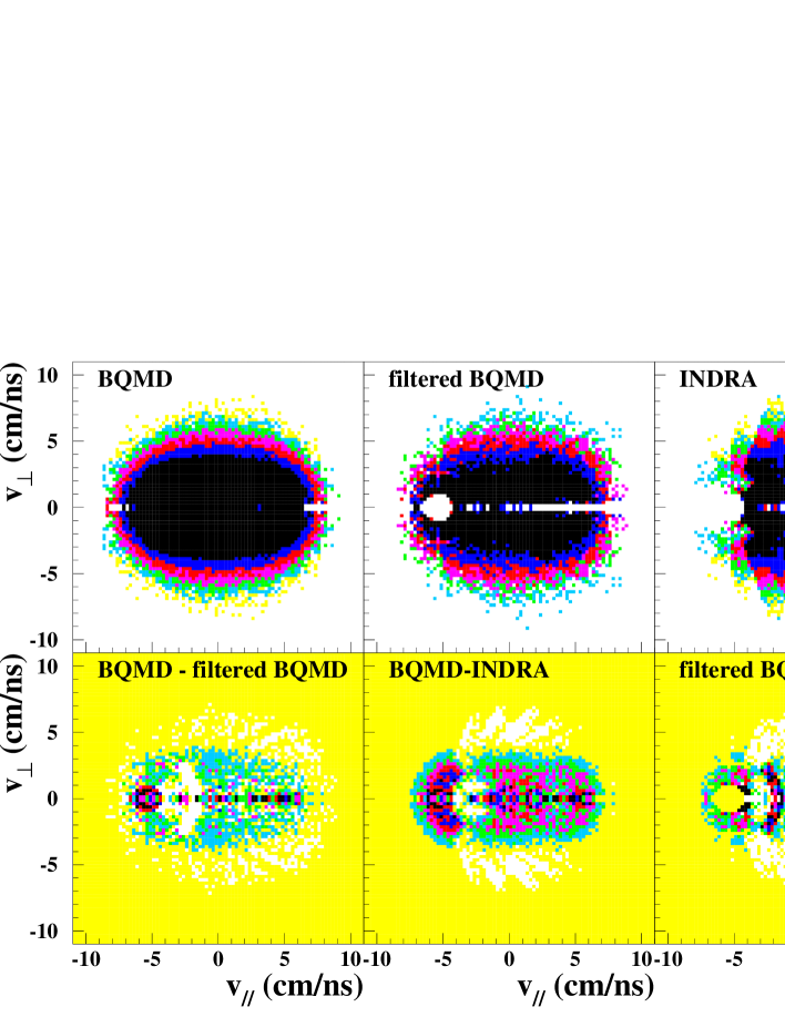
Figure 1: Comparison of non filtered (top left) and filtered (top middle) QMD distributions for Z=3 particles for the two most central bins with experimental results (top right) for the reaction Au+Au at 60 AMeV. In order to show how the filter modifies the events we display the difference between unfiltered and filtered QMD events (bottom left), between unfiltered simulations and experiment (bottom middle), as well as between filtered simulations and experiment (bottom right).

The influence of the filter on fragment yields is usually much larger than on light charged particles. How the filter modifies the raw simulation data on fragments is shown in fig.1 where we display the yield of central Au+Au reactions at 60 AMeV, the most critical energy, in the transverse velocity / longitudinal velocity plane in the center of mass, for particles with Z=3. Only those events in which the total observed charge $Z_{tot}$ is larger than 78% of the total charge of projectile and target are considered here. The top left (middle) figure shows the simulation events before (after) we have applied the INDRA filter. Top right one sees the experimental results. The suppressed particles are displayed in the left bottom part of the plot. We see that the filter suppresses particles in the entire $v_{long}-v_{trans}$ plane. On the first view this is astonishing because usually one expects that in forward direction the large majority of particles is seen in the detectors. The suppression is strongest at small transverse momenta. The difference between filtered events and data is displayed in the figure bottom right. Although the filtered QMD events give a fragment distribution which comes closer to the INDRA data than the unfiltered events (compare the middle and right figures in the bottom row) the agreement is not at all perfect. We see that in the simulations there are too many fragments. The excess is concentrated along an ellipse around midrapidity. This surplus appears at relatively high center of mass energies. This effect is especially pronounced for heavy fragments. There the filter creates fragments close to the beam velocity. Therefore, if one averages over all events, the filtered simulation events show less stopping than the true events. In view of the above discussion this is due to too little stopping in the simulations in this heavy system subsequently amplified by the filter. This lack of stopping has not been observed for the smaller Xe+Sn system at 50 AMeV reg . The filter suppresses many more fragments with negative center of mass velocity ($v_{cm}$) than with positive $v_{cm}$. Hence the filtered QMD events are no longer symmetric. Because, as we will see later, the simulation events produce very well the $E_{trans12}$ distribution ($E_{trans12}$ is the total transverse energy of all particles with charge Z= 1,2) and hence the number of hard NN scatterings this lack of stopping is due to the mean field. Therefore the fragment pattern will not be influenced substantially.

In the past, theoretical results for a given impact parameter have often been directly compared with data which have been selected according to their multiplicity or transverse energy amdind . This may yield, as we show now, erroneous results. In the experiment, the most central events are selected by requiring that $E_{trans12}>1246(3313)$ MeV at 60 (150) AMeV which corresponds to a cross section of $\sigma=\pi$(1fm)${}^{2}.$. Because of the finite resolution in impact parameter, the so-defined event class is different from the truly most central events with $b\leq 1$ fm which give the same cross section (fig.2).

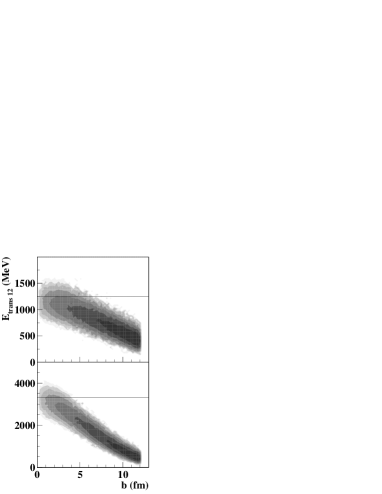
Figure 2: The correlation between impact parameter and $E_{trans12}$ for Au+Au reactions at 60 AMeV (top) and 150 AMeV (bottom) according to the QMD. The events above the cut in $E_{trans12}$ correspond to a geometrical cross section of $\sigma=\pi$(1fm)${}^{2}.$

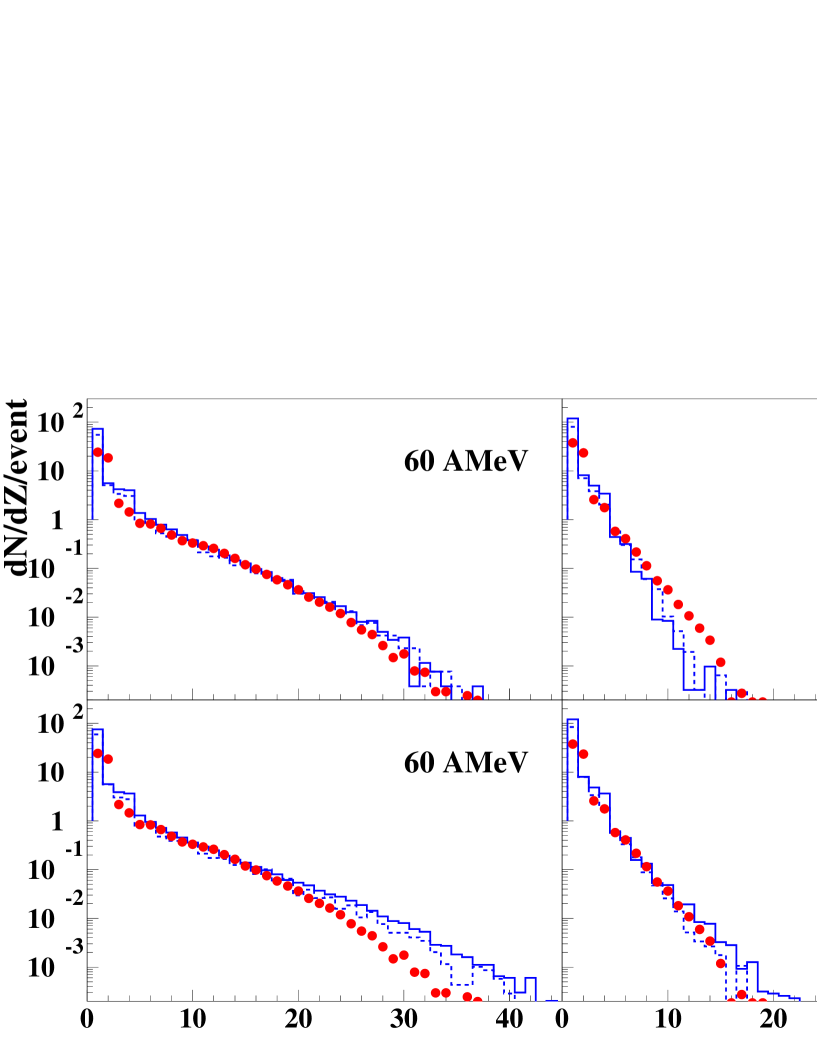
Figure 3: The fragment yield of simulated events with $b\leq 1$ fm (top) and $E_{trans12}\geq 1246(3313)$ MeV (bottom) for Au+Au reactions as compared to the experimental data which have been selected by $E_{trans12}$. Full (dashed) lines correspond to unfiltered (filtered) QMD events.

Therefore it is not astonishing that physical quantities for the two different choices of centrality differ as well. As an example we present in fig. 3 the fragment distributions for the reaction Au+Au at 60 AMeV and 150 AMeV. With decreasing $E_{trans12}$ a smaller number of violent nucleon-nucleon collisions have taken place and therefore heavier fragments can survive. We see therefore a less steep fragment yield for the $E_{trans12}$ selection than for the impact parameter selection, especially for the large fragments. The number of binary collisions is inversely correlated with the impact parameter and therefore also the probability that the initial-final state correlations, which will be discussed in section IX, become destroyed. The figure shows that quantitative comparisons require a cut in a variable which is experimentally accessible. As we will see later, in the reaction at 60 AMeV, projectile and target form almost a compound system although in momentum space the equilibration is not perfect. Consequently, at the end of the calculation the nucleons remain very close in coordinate space. This makes it very difficult to determine the fragments in the simulation events and the systematical error is much larger than at higher energies where the fragments are clearly separated in coordinate space at the end.

IV global event structure

Figure 4: The transverse energy distribution $dN/E_{trans12}$ for Au+Au reactions at 60 AMeV (left) and 150 AMeV (right). The full line are the unfiltered the dashed line the filtered QMD results. The QMD results are compared with the data. The vertical lines show the experimental centrality cuts for central events.

In the analysis of the Au+Au reaction the energy of light particles (Z= 1,2) ($E_{trans12}$) has been used for the event selection luk . This differs from the event selection criteria applied by the FOPI collaborations for the same reactions. We have, therefore, first of all, to check whether we can reproduce that quantity. If not, it will not be meaningful to compare the simulations with the INDRA data for selected centrality bins. In fig.4 we display the ($E_{trans12}$) distributions, for unfiltered (full line) and filtered (dashed line) QMD events as well as for the INDRA data. The normalization is arbitrary because in our simulation the maximal impact parameter is $b_{max}=12$ fm. The transverse energy distribution of semi-peripheral and central collisions are well reproduced. Please note that the $E_{trans12}$ distribution is also modified by the filter: The filter reduces $<E_{trans12}>$ by 13 (23)% at 60 (150) AMeV.

V Fragment distributions, multiplicities and spectra

After having seen that the transverse energy distribution of the light charged particles in the filtered simulations agrees well with that of the INDRA data the next question is whether also fragments are reasonably reproduced. In figs. 5 and 6 we display the multiplicity distribution of

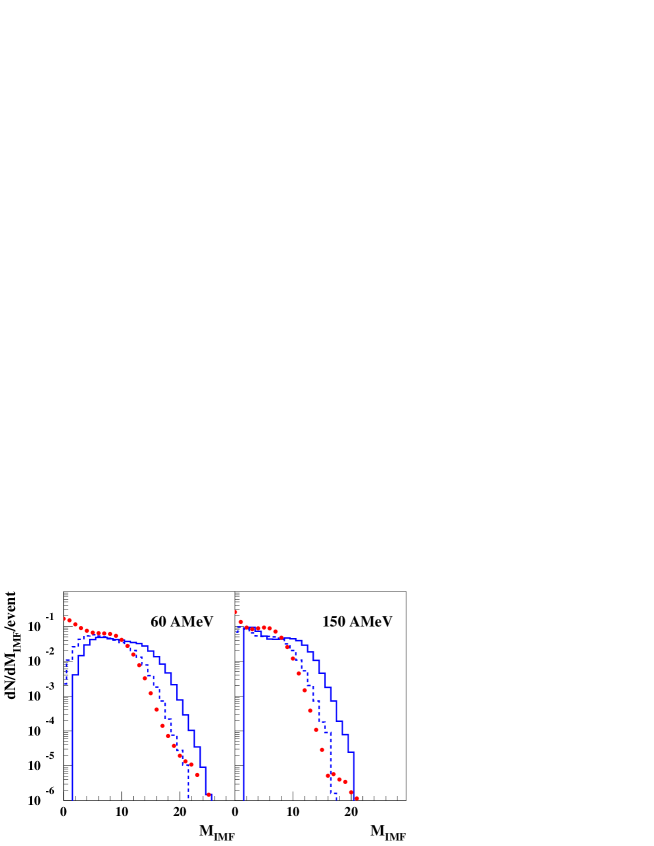
Figure 5: Multiplicity distributions of intermediate mass fragments. We compare for all events unfiltered (full line) and filtered (dashed line) QMD simulations with Au+Au data (60 AMeV left and 150 AMeV right).

intermediate mass fragments ($3\leq Z\leq 25$). Fig.5 displays the distribution for all impact parameters, fig.6 shows the distribution for central events selected according to the experimental cut in $E_{trans12}$. These central events correspond to a geometrical cross section of 3.14 fm². We see, first of all, that the filter reduces the fragment multiplicity considerably and brings the distribution close to the experimental one. In fig.5 one sees the lack of events with a low multiplicity, a consequence of the fact that we have stopped the simulations at b=12 fm. For central Au+Au reactions at 60 AMeV the filtered QMD events give the right form of the distribution but over-predict slightly the multiplicity. At 150 AMeV the form as well as the absolute value is well reproduced. Fig.8 shows the fragment yield and fig.8 the charge of the heaviest fragment for central reactions in Au+Au at 60 AMeV (top), 100 AMeV (middle) and 150 AMeV (bottom). Again we see that these distributions are well described at 100 and 150 AMeV despite the considerable changes of this distribution between these two energies. At 60 AMeV we see that we overpredict the fragment yield above Z= 25. This points once more to the difficulty to identify the medium mass fragments in the simulations at this energy due to their very small relative momentum.

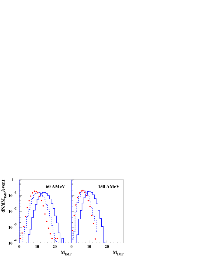
Figure 6: Multiplicity distribution of intermediate mass fragments. We compare for central events unfiltered (full line) and filtered (dashed line) QMD simulations with data (60 AMeV left and 150 AMeV right).

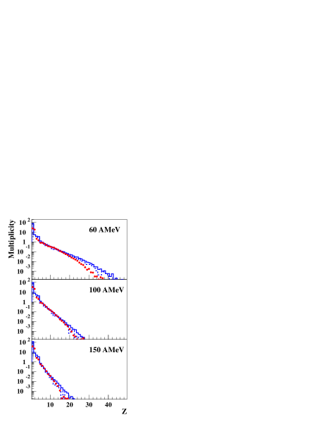
Figure 7: Fragment distribution. We compare for central events unfiltered (full line) and filtered QMD (dashed) simulations with data.

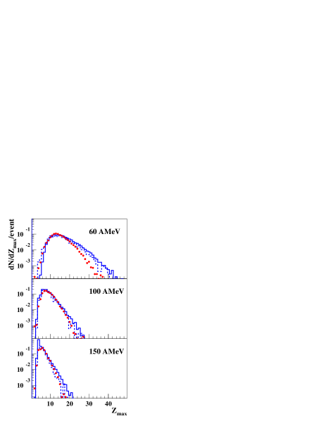
Figure 8: Distribution of the heaviest fragment. We compare for central events unfiltered (full line) and filtered QMD (dashed) simulations with data.

The energy distribution for the Z=3 and Z=5 fragments is shown in fig.9 for 60 AMeV and 150 AMeV. The slope is well reproduced by the QMD simulation in all cases but deviations occur at small $E_{cm}$ energies for Z=5 at 150 AMeV. Experimentally the peak is close to the Coulomb barrier, whereas in the simulations the fragments are less stopped. This transparency is also seen for larger fragments.

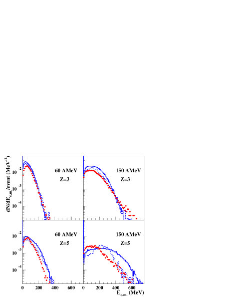
Figure 9: Energy distribution of Z=3 and Z=5 fragments from central events, left for 60 AMeV, right for 150 AMeV.

VI Is there an equilibrated source in central collisions?

As said in the introduction, there are two different approaches to

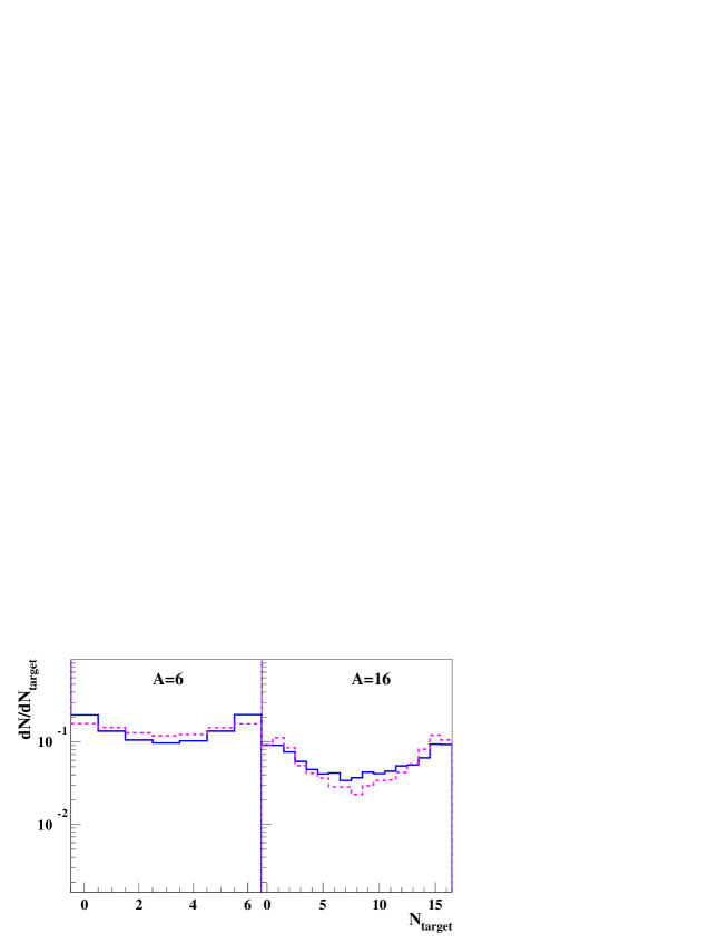
Figure 10: QMD prediction for the composition of fragments in terms of nucleons which have been initially in the target for A=6 (left) and and A=16 (right) in central Au+Au collisions ($b\leq 3\$fm). The full(dashed) line shows the distribution for 60 (150) AMeV.

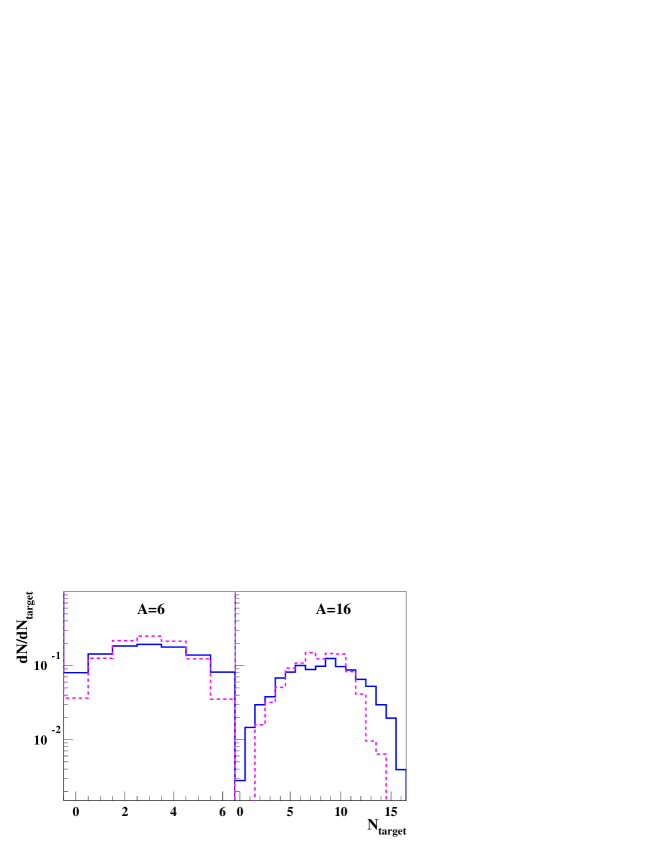
Figure 11: QMD predictions for the composition of mid-rapidity fragments in terms of nucleons which have been initially in the target for A=6 (left) and A=16 (right) in central Au+Au collisions ($b\leq 3\$ fm). The full(dashed) line shows the distribution for 60 (150) AMeV.

describe multifragmentation. If the statistical picture were correct, we would expect that in central collisions the nucleons in a fragment come in almost equal parts from projectile and target. For the system 50 AMeV Xe+Sn, the dynamical calculations showed that fragments are dominated either by projectile or by target nucleons and only in rare cases fragments are formed in which both are present with about the same weight goss .

Figure 12: QMD predictions of the correlation between the fraction of entrained target nucleons and the longitudinal fragment velocity in the center of mass for fragments with $6\leq Z\leq 10$ in central Au+Au reactions

This situation is different for the heavier Au+Au system. Fig.10 shows that in central collisions fragments of every mixture of projectile and target nucleons can be observed. Thus there exist fragments with the same number of projectile and target nucleons. This is true for both energies and for different fragment sizes. If we concentrate on fragments which are finally observed at midrapidity ($60^{\circ}\leq\theta_{cm}\leq 120^{\circ}$), fig.11, we see this effect to be enhanced.

Figure 13: $R=\frac{<y^{2}x>}{<y^{2}z>}$ as a function of the fragment charge for central events in Au +Au reactions at 150 AMeV measured by the INDRA and the FOPI collaboration info . The data are compared with the results of the QMD calculation.

Here fragments composed of a similar number of projectile and target nucleons dominate. Thus central Au+Au collisions show complete mixing and therefore statistical models can be employed to study the fragment yields or fragment multiplicities. Does this mean that the system has also reached equilibrium in the dynamical variables? To study this question we investigate the correlation between the composition of a fragment and its velocity in the center of mass system. If equilibrium had been obtained we would see a flat distribution because in equilibrium all nucleons have the same distribution independent of their origin. The result of the QMD calculations, displayed in fig.12, shows, on the contrary, a strong correlation even at midrapidity where complete mixing has been observed. Thus the dynamical degrees of freedom have not attained equilibrium.

To look further into this question we calculate the mean squared rapidity variances in the impact parameter direction, $<y^{2}_{x}>$, and in longitudinal direction, $<y^{2}_{z}>$ for Au+Au at 150 AMeV. In a system in which the dynamical degrees of freedom are equilibrated we expect a ratio $R={<y^{2}_{x}>}/{<y^{2}_{z}>}=1.$ QMD as well as both experiments, FOPI and INDRA, show that global thermalization is not achieved. Fig.13 displays the results. We see that protons are close to an equilibrium in the dynamical variables $(R\approx 0.9)$ but for fragments the value of R is well below 1. Even more, the ratio is a function of the fragment charge and decreases rapidly. In QMD this is understandable: As we will see the majority of fragments are surviving initial state correlations and the fragments are not decelerated substantially in longitudinal direction. Therefore their kinetic energy is, in first approximation, proportional to their atomic number A. In terms of purely thermal models this means that the source properties depend on the fragments mass. In order to make two independent 4$\pi$ experiments comparable info , both, the ALADIN/INDRA as well as the FOPI group, have made substantial efforts to determine the most central events. To determine central events one plots all events as a function of a certain centrality definition ($E_{rat},E_{trans12}..$) and takes then those events with corresponds to a cross section $\sigma<\pi\cdot 4$ fm² assuming that the total reaction cross section is known. It is impossible to model this criterion precisely in QMD. Therefore we have taken in the QMD events an impact parameter cut of $b=2$ fm (see fig. 3).

VII Bi-modality

If a finite system undergoes a first order phase transition bi-modality Fran is observed. It may even exist if a sizable fraction of the initial momentum is not relaxed fg as it is the case in heavy ion reactions. Bi-modality in systems with a phase transition means that for the same value of the control parameter the two phases, the ordered (liquid) and disordered (gas) one, are present. Experimentally, the control parameter of the phase transition is very difficult to access, if at all, and so one has to connect it to some experimentally observable quantity.

In order to study whether a liquid-gas phase transition can be observed in heavy ion reactions it has been suggested in ref. tam to study quasi-projectile decay sorted by quasi-target temperature, estimated from the total transverse energy of light particles emitted at backward angles in the c.m. frame. If a system is bi-modal in the same event class a liquid-like phase (events with one large fragment) and a gas-like phase (events with no large fragment) co-exist.

To quantify the bi-modality one may define as in ref. tam

$$a_{2}=(Z_{max}-Z_{max-1})/(Z_{max}+Z_{max-1})$$ (1)

where $Z_{max}$ is the charge of the largest fragment, while $Z_{max-1}$ is the charge of the second largest fragment, both observed in the same event in the forward hemisphere. If the system shows bi-modality we will observe in the same event class two types of events: One with a large $a_{2}$ (one big fragment with some very light ones) the other with small $a_{2}$ (two similarly sized fragments). Events with intermediate values of $a_{2}$ should be rare.

In the INDRA Au+Au experiments bi-modality has been indeed observed: In the same $E_{trans12}$ bin the distribution of the largest fragment shows two well separated maxima and $a_{2}$ as a function of $E_{trans12}$ varies very rapidly tam . The question is whether this observation can only be explained by a phase transition in a finite size system or whether alternative explanations can be advanced.

As will be discussed in a separate paper, simulation programs like QMD show as well bi-modality lza . As an example we display in fig. 14 $Z_{max}$ for filtered events at 150 AMeV. We made sure that also the unfiltered events have qualitatively the same structure. The bin $1419$ MeV $\leq E_{trans12}<1892$ MeV shows the presence of two types of events with quite different $Z_{max}$ as may be inferred from the right figure in the bottom row.

Figure 14: $Z_{max}$ as a function of the asymmetry parameter for the different experimental centrality bins for filtered QMD events at 150 AMeV.

If one studies the origin of the bi-modality in QMD simulations one realizes that at large impact parameters the momentum transfer between projectile and target is not sufficient to decelerate the nuclei substantially. At the end of the reaction we find two excited heavy remnants. At small impact parameters the stopping is not complete but the decelerated projectile and target remnants do not separate anymore. They remain connected by a bridge of matter from nucleons originating from the overlap zone as will be discussed in section VIII. At the end of the reaction this connected matter fragments. The break points are given by local instabilities. Therefore small fragments of quite different sizes are formed. This general behavior, that between projectile and target a bridge of matter is formed in heavy ion collisions at intermediate impact parameters has already been found in BUU calculations abuu .

The transition between the two reaction scenarios is rather sharp. Therefore we see a sudden increase of the $a_{2}$ value if we increase the impact parameter (fig. 15 right). Because the stopping and the impact parameter are strongly correlated we observe a similar increase if we plot $a_{2}$ as a function of $E_{trans12}$ as shown in fig. 15 left. Due to the increase of the nucleon-nucleon cross section with energy for a given impact parameter the momentum transfer depends on the beam energy . Therefore the value of b for which this transition takes place varies with the beam energy. On the contrary, the value of $E_{trans12}$, which measures directly the energy transfer, remains constant as observed also in the INDRA experiments.

Figure 15: The most probable $a_{2}$ in unfiltered QMD simulations as a function of $E_{trans12}/E_{cm}$ (left) and as a function of the impact parameter (right). As in experiment we see in both cases a fast transition.

VIII The Dynamics of the Reaction

VIII.1 Transition between participant and spectator fragmentation

To study the evolution of the reaction mechanism from participant to spectator dominated multifragmentation we use semicentral reactions $6\leq b\leq 8$ fm and medium mass fragments ($10\leq A\leq 20$). For this purpose we use now the fact that in the QMD simulations one knows the position and momentum of all particles at any given time point and therefore it is possible to study the history of those nucleons which are finally part of the different fragments. The color coding shows where the nucleons are, independent of whether these nucleons will finally be part of a fragment. The size of the squares gives the percentage of the nucleons (as compared to all nucleons) which end up finally in fragments of the selected class (here $10\leq A\leq 20$). We plot these both distributions for different time steps, on the right hand side for the reaction at 60 AMeV and on the left hand side for 150 AMeV in fig. 16. This figure is supplemented by fig. 17 which shows the initial and final momentum distribution using the same coding. We see, first of all, that at both energies the initial distribution of those nucleons which end finally up in fragments is different from that of all nucleons. This means that strong initial-final state correlations are present which we study now in detail.

Figure 16: QMD predictions of the distribution of all nucleons (colors) and those nucleons which belong finally to a fragment $\textrm{10}\leq A\leq\textrm{20}$ (boxes) for collisions $6\geq b\geq$8 fm for Au + Au at 150 AMeV (left) and 60 AMeV (right) from t= 0 (top) to t=200 fm/c(bottom)

Figure 17: QMD prediction of the momentum space distribution of all nucleons (colors) and those nucleons which belong finally to a fragment $\textrm{10}\leq A\leq\textrm{20}$ (boxes) for collisions $6\geq b\geq$8 fm for Au + Au at 150 AMeV (left) and 60 AMeV (right) at t= 0 (top) and t=200 fm/c(bottom)

In coordinate space the nucleons which form finally fragments $10\leq A\leq 20$ are located toward the reaction partner. At 150 AMeV one sees clearly that they come from the spectator matter. The time evolution for both energies is rather different and best seen if one compares the positions at 80fm/c of 60 AMeV with those at 40fm/c of 150 AMeV. At 60 AMeV we observe neck formation as at lower energies and the future fragment nucleons are concentrated in the neck, i.e. in the center of the reaction. At 150 AMeV the nucleons show a completely different behavior. The future fragment nucleons are those which are not in the geometrical overlap of projectile and target. This is a clear indication that between 60 AMeV and 150 AMeV the transition between participant and spectator fragmentation takes place, a transition which was believed to take place at considerably higher energies and has been observed at energies above 400 AMeV Schuet .

In addition to the initial-final state correlations in coordinate space, there are also similar correlations in momentum space. At 150 AMeV future fragment nucleons have a transverse momentum away from the reaction zone (and thus the observed transverse fragment velocity is partially due to the selection of the fragment nucleons neba ). At 60 AMeV the correlation are less important but nucleons with a smaller longitudinal momentum have a higher chance to be part of a IMF than those with a larger longitudinal momentum.

Figure 18: Momentum space distribution of all nucleons (colors) and those nucleons which belong finally to a fragment $1\textrm{0}\leq A\leq\textrm{20}$ (boxes) for central collisions $0\geq b\geq 4$ fm for Au + Au at 150 AMeV (left) and 60 AMeV (right) at t= 0 (top) and t=200 fm/c (bottom).

Central collisions are rather similar to the semicentral ones at both energies. Again the fragment nucleons come dominantly from the overlap zone at 60 AMeV and from the spectator matter at 150 AMeV. Therefore we show only the momentum space distributions which are displayed in fig.18. The average deceleration is of course much stronger as compared to the semicentral reactions but the fragments at 150 AMeV, coming from the spectator matter, are less influenced by this. They have still a quite large momentum. However, the matter at midrapidity is now that dense that some fragments are created forming the midrapidity source discussed above. The in-plane flow seen in semicentral collisions has almost disappeared, as expected.

Figure 19: Multiplicity of intermediate mass fragments as a function of the impact parameter for Au+Au reactions at 60 AMeV, 100 AMeV and 150 AMeV. The full (dashed) line shows unfiltered (filtered) QMD events.

This transition between participant and spectator fragmentation is also visible if one plots the multiplicity of IMF’s as a function of the impact parameter, as done in fig. 19. Whereas at 60 AMeV the multiplicity peaks at $b=0$, at 150 AMeV semicentral events show a higher multiplicity. The filter modifies this observation which agrees with the data tsang ; luka only slightly.

VIII.2 Small IMF’s come from many sources

For semicentral collisions the initial-final correlations of those nucleons which end up in $1\textrm{0}\leq A\leq\textrm{20}$ fragments are almost identical to that of $\textrm{6}\leq A\leq\textrm{10}$ fragments. Therefore we do not display them. A difference can be observed in central collisions. The time evolution in coordinate space is presented in fig.20 whereas that in momentum space is presented in fig.21.

Figure 20: Distribution of all nucleons (colors) and those nucleons which belong finally to a fragment $\textrm{6}\leq A\leq\textrm{10}$ (boxes) for central collisions $0\geq b\geq 4$ fm for Au + Au at 150 AMeV (left) and 60 AMeV (right) from t= 0 (top) to t=200 fm/c (bottom)

Figure 21: Momentum space distribution of all nucleons (colors) and those nucleons which belong finally to a fragment $\textrm{6}\leq A\leq\textrm{10}$ (boxes) for central collisions $0\geq b\geq 4$ fm for Au + Au at 150 AMeV (left) and 60 AMeV (right) at t= 0 (top) and t=200 fm/c(bottom)

Here, at 150 AMeV, in addition to the fragments from the spectator matter a midrapidity source develops (seen clearly in the second row of fig.20) which finally creates a bridge between target and projectile spectator fragments, seen in the bottom row, similar to what we have seen for large fragments at 60 AMeV. This is reflected, of course, in momentum space (fig.21) where we see - in contradistinction to the $1\textrm{0}\leq A\leq\textrm{20}$ data - a midrapidity source. It has never been observed before in simulations of smaller systems that this midrapidity source, which reminds on the neck formation at lower energies, emits fragments of this size. Also the initial-final state correlations in coordinate space are much weaker than for the larger fragment class, $1\textrm{0}\leq A\leq\textrm{20}$. We see that quite a few of these fragments come from the participant matter.

IX How fragments can survive the high density zone

In section VI we have seen that part of the fragments are made of nucleons which have traversed the reaction zone. How this can happen we have shown in ref. goss for the system Xe+Sn. There we have found that fragments are made of nucleons which have passed the reaction zone without having had collisions with a large transverse momentum transfer. Nucleons with similar momenta which are close in coordinate space suffer the potential interaction in the same way and therefore are collectively deviated by potential gradients. Therefore they leave collectively the interaction zone without the initial correlation among them being destroyed. Therefore in QMD calculations fragments at forward and backward rapidity present those initial state correlations which have not been destroyed by hard binary collisions. If these collisions become more frequent, for example by increasing the beam energy and by this reducing the influence of the Pauli blocking, less fragments are observed, because more of the initial state correlations have been destroyed.

Here we explore whether this mechanism remains valid even for the large Au+Au system. To study this question we make use of the fact that we know the position and momentum of all nucleons during the whole reaction. This allows to trace back the history of all nucleons and especially of those which are finally part of a fragment i which contains A nucleons. For these nucleons we define three quantities, the average momentum

$$\vec{P}^{i}(t)=\frac{1}{A}{\displaystyle\sum_{j=1}^{A}}\vec{p}_{j}(t),$$ (2)

the position of the center of mass of the fragment

$$\vec{R}^{i}(t)=\frac{1}{A}{\displaystyle\sum_{j=1}^{A}}\vec{r}_{j}(t),$$ (3)

and the average transverse (with respect to the beam momentum) kinetic energy of the fragment nucleons in the fragment rest system

$$\Delta^{i}(t)={\displaystyle\sum_{j=1}^{A}}\frac{(p_{j}^{\perp}(t)-P^{i\perp}(t))^{2}}{2m{A}}.$$ (4)

$\Delta^{i}(t)$ is sometimes sloppily called ”fragment temperature”. The finite value at t = 0 is due to the Fermi motion. We compare now this ”fragment temperature” with the environment. The environment is defined by those nucleons which are at the same time closer than 2.5 fm to the center of the fragment $\vec{R}^{i}(t)$ and also are not belonging to the fragment i. For those nucleons we define as well the average kinetic energy

$$\Delta^{env}_{i}(t)={\displaystyle\sum_{j=1}^{B}}\frac{(p_{j}^{\perp}(t)-P^{i\perp}_{env}(t))^{2}}{2m{B}}.$$ (5)

$P^{i\perp}_{env}(t)$ is the mean transverse momentum of the B nucleons of the environment. The number of nucleons in the environment changes during the reaction. At the very end of the reaction there is usually no nucleon left in the environment because all fragments and single nucleons are well separated in coordinate space. $\Delta^{env}_{i}(t)$ can sloppily be called ”temperature of the environment”. If the fragments are only created at freeze out when the system is in thermal equilibrium we would expect that before freeze out there is no difference between the “fragment temperature” and the “temperature of the environment”. This is due to the very fundamental fact that if a system is in thermal equilibrium all two or more body correlations are lost and therefore eventually existing correlations before freeze out cannot play a role for the production of the fragments at freeze out. In other words, every nucleon has the same chance to be finally part of the fragment i and therefore the nucleons of the environment and the fragment nucleons should have the same properties.

The result of the simulations, averaged over all M fragments i of the size Z = 3, is displayed in fig 22. We see a quite different time evolution of $\Delta$ and $\Delta^{env}$. When passing the reaction zone, where the density is high, $\Delta^{env}$ increases strongly whereas $\Delta$ remains almost constant. The fragment nucleons do not take part in the heating of the system. At the end of the reaction $\Delta^{env}$ becomes smaller because the high relative momentum particles have already left the environment. Only at the end of the reaction $\Delta$ increases because the fragments leave the interaction zone with a deformed shape, as can be directly seen in the simulations. By regaining their spherical shape the (negative) binding energy increases and - due to energy conservation - the (positive) kinetic energy of nucleons in fragments has to increase as well in order to conserve the total energy. At this late stage the fragments are separated, there are no environment nucleons around, therefore the ”temperature of the environment” is 0. Thus we see that the mechanism we have found for the smaller Xe+Sn system goss is still valid for the large Au+Au system. The mean free path of the Pauli blocked cross section for large transverse momentum transfer is still well below the diameter of the system and therefore initial-final state correlations can survive.

Figure 22: Time Evolution of the central density, of $\Delta$ and of the binding energy Ep of Z=3 fragments during the reaction.

X conclusion

Using the QMD model we have investigated multifragmentation data in Au+Au reactions between 60 AMeV and 150 AMeV obtained by the INDRA collaboration. We observe that in this energy range the transition between fragmentation of participant matter and fragmentation of spectator matter takes place. We see for the first time that midrapidity fragments are dominantly formed of an equal number of projectile and target nucleons, as required if the system comes to equilibrium. This explains the success of statistical approaches in reproducing particle multiplicities in this phase space region. This mixing appears although the particle momentum does not equilibrate. Nucleons coming from the projectile (target) carry still a fraction of their initial collective momentum, especially if they end up in fragments. In fragments at midrapidity, which on average contain the same number of nucleons from projectile and target, these ”memory effects” compensate and do not influence the fragment momentum. Free nucleons come closest to equilibrium because in order to be free they have usually suffered collisions with a large momentum transfer. A common source of all fragments cannot be identified, the source properties depend on the fragment size. This observation has been confirmed now independently from the data of the INDRA and the FOPI collaboration. Without passing through a filter theory and experiment cannot be compared. After filtering the QMD simulations describe well the energy dependent event centrality, the multiplicity distribution of fragments, the fragment yield and the distribution of the largest fragment. It describes as well the energy distribution of the smaller fragments. Even for this large system, forward emitted fragments are initial state correlations in coordinate and/or momentum space which are not destroyed during the reaction by collisions with a large momentum transfer, similar to the observations for much smaller systems. Thus for the largest system explored so far, the system comes close to equilibrium but non-equilibrium effects still dominate outside a small midrapidity zone.

References

- (1) A LeFèvre et al. Nucl. Phys. A735 (2004) 219.
-
(2)
J. Łukasik it et al. PLB 566 (2003) 76;
J.D. Frankland et al. Phys. Rev. C71 034607 (2005). - (3) G.J. Kunde at al, Phys. Rev. Lett 74, 38 (1995)
- (4) M.E. Fischer, Physics 3, 255 (1967).
- (5) J.P. Bondorf, A.S. Botvina, A.S. Iljinov, I.N. Mishustin, K. Sneppen, Phys. Rep. 257 133 (1995).
- (6) D.H.E. Gross, Rep. Prog. Phys. 53, 605 (1990), and references therein.
- (7) D. Hahn and H. Stöcker, Nucl. Phys. A 476, 718 (1988).
-
(8)
J. Aichelin and J. Hüfner,
Phys. Lett. B 136 (1984) 15;
J. Aichelin, J. Hüfner, and R. Ibarra Phys. Rev. C 30 (1984) 107. - (9) A.S. Goldhaber Phys. Lett. B53 (1974) 306.
- (10) C. Hartnack et al., Phys. Lett. B506 261 (2001).
- (11) J. Aichelin, Phys. Rep. 202 (1991) 233.
- (12) C. Hartnack et al. Eur. Phys. J. A 1 (1998) 151.
- (13) R. Nebauer et al. Nucl. Phys. A658, 67 (1999).
- (14) A. Ono, H. Horiuchi Phys. Rev. C53, 2958 (1996).
- (15) A. Ono et al., Phys. Rev. C 66, 014603 (2002).
-
(16)
Y. Abe, S. Ayik, P.G. Reinhard, E. Suraud, Phys.Rep. 275, 49
(1996)
S. Ayik, E. Suraud, M. Belkacem, D. Boilley, Nucl.Phys. A545, 35C (1992)
Akira Ohnishi, Jorgen Randrup, Phys.Lett. B394, 260 (1997)
A. Guarnera, P. Chomaz, M. Colonna, J. Randrup, Phys.Lett.B403, 191 (1997) -
(17)
D. Cussol and O. Lopez, privat communication;
A. Trzcinski et al. Nucl. Instr. and Meth. A501 (2003) 367;
J. Pouthas et al., Nucl. Instrum. Methods A357, 418 (1995);
J. Pouthas et al., Nucl. Instrum. Methods A 369, 222 (1996). -
(18)
J. Lukasik et al., Phys. Lett B608, 223 (2005);
W. Trautmann et al., in Proceedings of XLII International Winter Meeting on Nuclear Physics, Bormio, Italy, 2004, ed. by I. Iori, Ricerca Scientifica ed Educazione Permanente Suppl. #123 (Milano 2004), p. 272; nucl-ex/0404025. - (19) P.B. Gossiaux and J. Aichelin, Phys. Rev. C56 (1997) 2109.
- (20) A. Andronic, J. Łukasik, W. Reisdorf, and W. Trautmann, to be published in Eur. Phys. J. A.
- (21) Ph. Chomaz, F. Gulminelli, Physica A 330, 451 (2003).
- (22) F. Gulminelli and Ph. Chomaz, Nucl. Phys. A734, 581 (2004).
-
(23)
M. Pichon et al. (INDRA collaboration), Nucl. Phys. A 749
(2004) 93c;
M. Pichon et al. (INDRA collaboration), nucl-ex/0602003. - (24) A. LeFèvre, K. Zbiri and J. Aichelin, to be published.
- (25) J. Aichelin, Phys. Lett. B 175, 120 (1986).
- (26) M.B. Tsang et al., Phys. Rev. Lett 71, 1502 (1993).
- (27) J. Łukasik et al., Phys. Lett. B566 ,76 (2003).
- (28) A. Schüttauf et al., Nucl. Phys. A607, 457 (1996)
-
(29)
R. Nebauer et al., Nucl. Phys. A650, 65 (1999);
C. Hartnack et al., Phys. Rev. C56, 2109 (1994).