Eccentricity fluctuations and elliptic flow at RHIC

Abstract

Fluctuations in nucleon positions can affect the spatial eccentricity of the overlap zone in nucleus-nucleus collisions. We show that elliptic flow should be scaled by different eccentricities depending on which method is used for the flow analysis. These eccentricities are estimated semi-analytically. When $v_{2}$ is analyzed from 4-particle cumulants, or using the event plane from directed flow in a zero-degree calorimeter, the result is shown to be insensitive to eccentricity fluctuations.

1. Introduction

Elliptic flow, $v_{2}$, is one of the key observables in nucleus-nucleus collisions at RHIC Ackermann:2000tr . It originates from the almond shape of the overlap zone (see Fig. 1) which produces, through unequal pressure gradients, an anisotropy in the transverse momentum distribution Ollitrault:1992bk , the so-called $v_{2}\equiv\left\langle\cos 2\phi\right\rangle$, where $\phi$’s are the azimuthal angles of the detected particles with respect to the reaction plane.

Preliminary analyses of $v_{2}$ in Cu-Cu collisions at RHIC  Masui:2005aa ; Manly:2005zy ; Wang:2005ab , presented at the QM’2005 conference, reported values surprisingly large compared to theoretical expectations, almost as large as in Au-Au collisions. It was shown by the PHOBOS collaboration Manly:2005zy that fluctuations in nucleon positions provide a natural explanation for this large magnitude. The idea is the following: The time scale of the nucleus-nucleus collision at RHIC is so short that each nucleus sees the nucleus coming in the opposite direction in a frozen configuration, with nucleons located at positions whose probabilities are determined according to the nuclear wave function. Fluctuations in the nucleon positions result in fluctuations in the almond shape and orientation (see Fig. 1), and hence in larger values of $v_{2}$.

In this Letter, we discuss various definitions of the eccentricity of the overlap zone. We show that estimates of $v_{2}$ using different methods should be scaled by appropriate choices of the eccentricity. We then compute the effect of fluctuations on the eccentricity semi-analytically to leading order in $1/N$, where $N$ is the mean number of participants at a given centrality. A similar study was recently performed by S. Voloshin on the basis of Monte-Carlo Glauber calculations Voloshin:2006gz .

2. Eccentricity scaling and fluctuations

Elliptic flow is determined by the initial density profile. Although its precise value depends on the detailed shape of the profile, most of the relevant information is encoded in three quantities: 1) the initial eccentricity of the overlap zone, $\varepsilon$, which will be defined more precisely below; 2) the density $n$, which determines pressure gradients through the equation of state (by density, we mean the particle density, $n$, at the time when elliptic flow develops; this time is of the order of the transverse size $R$. Quite remarkably, the density thus defined varies little with centrality, and has almost the same value in Au-Au and Cu-Cu collisions at the same colliding energy per nucleon Bhalerao:2005mm ); 3) the system transverse size $R$, which determines the number of collisions per particle. $v_{2}$ scales like $\varepsilon$ for small $\varepsilon$, that is, $v_{2}=\varepsilon f(n,R)$.

This proportionality relation is only approximate. However, hydrodynamical calculations Bhalerao:2005mm show that it is a very good approximation in practice for nucleus-nucleus collisions. Eccentricity scaling holds for integrated flow as well as for the differential flow of identified particles. In the latter case, the function $f(n,R)$ also depends on the mass, transverse momentum and rapidity of the particle.

Eccentricity scaling of $v_{2}$ is generally believed to be a specific prediction of relativistic hydrodynamics. In the form above, the scaling is expected to be more general: it does not require thermalization, as implicitly assumed by hydrodynamics. If thermalization is achieved, that is, if the system size $R$ is much larger than the mean free path $\lambda$, then the scaling is stronger: $v_{2}/\varepsilon$ no longer depends on $R$, but only on the density $n$ Bhalerao:2005mm .

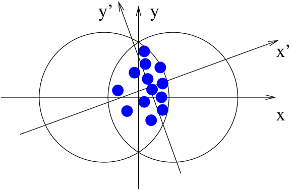
Figure 1: Schematic view of a collision of two identical nuclei, in the plane transverse to the beam direction ($z$-axis). The $x$- and $y$-axes are drawn as per the standard convention. The dots indicate the positions of participant nucleons. Due to fluctuations, the overlap zone could be shifted and tilted with respect to the $(x,y)$ frame. $x^{\prime}$ and $y^{\prime}$ are the principal axes of inertia of the dots.

The standard definition of the eccentricity is Sorge:1998mk

$$\varepsilon_{\rm s}=\frac{\left\langle y^{2}-x^{2}\right\rangle}{\left\langle y^{2}+x^{2}\right\rangle},$$ (1)

where $(x,y)$ is the position of a participant nucleon in the coordinate system defined in Fig. 1. Throughout this paper, $\left\langle...\right\rangle$ denotes an ensemble average: here, it means an average over participant nucleons and over many collision events of the same impact parameter. This standard eccentricity applies to most hydrodynamic calculations: indeed, most hydrodynamic calculations (with the exception of Ref. Socolowski:2004hw ) use smooth, event-averaged initial conditions, with an initial entropy density proportional to the density of participants Kolb:2003dz . The charged multiplicity then scales like the number of participants, as observed experimentally. (Adding a component proportional to the number of binary collisions, as argued in Kharzeev:2000ph , does not change the eccentricity significantly).

It was recently argued Drescher:2006pi that the Color Glass Condensate picture of heavy-ion collision leads to a different definition of the eccentricity, which may be significantly larger than the standard eccentricity. This interesting possibility will not be considered further here.

Now, because of the event-by-event fluctuations in the participant nucleon positions Miller:2003kd , the eccentricity driving elliptic flow in a given event is that defined by the principal axes $(x^{\prime},y^{\prime})$ of the distribution of participant nucleons, see Fig. 1. This “participant eccentricity” $\varepsilon_{\rm part}$ can be written as Manly:2005zy

$$\varepsilon_{\rm part}=\frac{\sqrt{(\sigma_{y}^{2}-\sigma_{x}^{2})^{2}+4\sigma_{xy}^{2}}}{\sigma_{y}^{2}+\sigma_{x}^{2}},$$ (2)

where

$$\sigma_{x}^{2} = \{x^{2}\}-\{x\}^{2}$$ (3)

$$\sigma_{y}^{2} = \{y^{2}\}-\{y\}^{2}$$ (4)

$$\sigma_{xy} = \{xy\}-\{x\}\{y\},$$ (5)

and $\{...\}$ denotes the average over all participants in one collision event (sample average). Our basic assumption in this paper is that in each event, the elliptic flow $v_{2}$ is proportional to the participant eccentricity $\varepsilon_{\rm part}$.

Experimentally, elliptic flow is analyzed by selecting events in a centrality class. The quantities which drive elliptic flow, namely, the density $n$, the transverse size $R$, the eccentricity $\varepsilon_{\rm part}$, fluctuate from one event to the other. This causes dynamical fluctuations of $v_{2}$. The effect of impact parameter fluctuations was carefully studied in Adler:2002pu and was shown to be small. In this paper, we focus on fluctuations in the positions of participant nucleons. It will be shown below that fluctuations in the eccentricity $\varepsilon_{\rm part}$ dominate over fluctuations in size and density.

3. To each method its own eccentricity

Since the reaction plane is not known exactly on an event-by-event basis, $v_{2}$ is measured indirectly using azimuthal correlations. Several methods have been used, which yield different estimates of $v_{2}$. We argue that these estimates are affected in different ways by fluctuations of $v_{2}$:

• The event-plane method Poskanzer:1998yz has been implemented by the STAR Ackermann:2000tr , PHOBOS Back:2002gz and PHENIX Adler:2003kt collaborations at RHIC. The event plane is an estimate of the reaction plane; it is defined as the plane spanned by the collision axis and the major axis of the ellipse formed by the transverse momenta of outgoing particles. It corresponds to the $x^{\prime}$ axis defined by the participants (Fig. 1), up to statistical fluctuations which are taken care of by the analysis (this is the so-called “event-plane resolution”). Outgoing particles are then individually correlated to this event plane. The corresponding estimate of $v_{2}$ will be denoted by $v_{2}\{{\rm EP2}\}$. Another method determines $v_{2}$ from two-particle azimuthal correlations between outgoing particles Adcox:2002ms . The corresponding estimate is usually denoted by $v_{2}\{2\}$, and is defined by an equation of the type $v_{2}\{2\}=\sqrt{\left\langle\cos 2(\phi_{1}-\phi_{2})\right\rangle}$. Both methods are essentially equivalent (see Sec. III.C.2 of Ref. Borghini:2000sa ). If $v_{2}$ fluctuates, both yield the rms value of $v_{2}$ Adler:2002pu : $v_{2}\{2\}\simeq v_{2}\{{\rm EP2}\}=\sqrt{\left\langle v_{2}^{2}\right\rangle}$. Since $v_{2}$ in each event scales with $\varepsilon_{\rm part}$, one expects $v_{2}\{2\}\simeq v_{2}\{{\rm EP2}\}\propto\varepsilon\{2\}$, where $\varepsilon\{2\}$ is defined by Miller:2003kd

  $$\varepsilon\{2\}\equiv\sqrt{\left\langle\varepsilon_{\rm part}^{2}\right\rangle}.$$ (6)

  This scaling differs from that proposed in Ref. Manly:2005zy , $v_{2}\propto\left\langle\varepsilon_{\rm part}\right\rangle$.

• Four-particle cumulants of azimuthal correlations Borghini:2001vi can be used to reduce the bias from nonflow correlations. The corresponding estimate of $v_{2}$ is denoted by $v_{2}\{4\}$. It involves a combination of 2-particle and 4-particle correlations, i.e., the 2nd and 4th moments of the distribution of $v_{2}$, $\left\langle v_{2}^{2}\right\rangle$ and $\left\langle v_{2}^{4}\right\rangle$. Assuming again that $v_{2}$ scales with $\varepsilon_{\rm part}$ in each event, one obtains $v_{2}\{4\}\propto\varepsilon\{4\}$, where $\varepsilon\{4\}$ is defined by Miller:2003kd :

  $$\varepsilon\{4\}\equiv\left(2\left\langle\varepsilon_{\rm part}^{2}\right\rangle^{2}-\left\langle\varepsilon_{\rm part}^{4}\right\rangle\right)^{1/4}.$$ (7)

• An alternative method determines the event-plane from directed flow Adams:2003zg , determined in a zero-degree calorimeter (ZDC) which detects spectator neutrons. Particles in the central rapidity region are then correlated to this event plane. This last estimate of $v_{2}$ is denoted by $v_{2}\{{\rm ZDC}\}$ Wang:2005ab . It differs from the previous ones in that the reference direction (the event plane) is determined by spectator neutrons from the projectile, rather than by participants. The direction defined by spectator neutrons is the $x$-axis, not the $x^{\prime}$-axis (see Fig. 1), up to fluctuations in spectator positions which are taken care of by the analysis. Therefore, the relevant eccentricity for this analysis is the reaction-plane eccentricity

  $$\varepsilon_{\rm RP}\equiv\frac{\sigma_{y}^{2}-\sigma_{x}^{2}}{\sigma_{y}^{2}+\sigma_{x}^{2}},$$ (8)

  and $v_{2}\{{\rm ZDC}\}$ should scale correspondingly like

  $$v_{2}\{{\rm ZDC}\}\propto\left\langle\varepsilon_{\rm RP}\right\rangle.$$ (9)

This estimate of $v_{2}$ is also unbiased by nonflow correlations because it involves a 3-particle correlation (instead of a 2-particle correlation in the standard event-plane method), and also because the ZDC calorimeter has a wide rapidity gap with the central rapidity detector.

4. Computing the fluctuations

We now compute the eccentricities entering Eqs. (6), (7) and (9), namely, $\varepsilon\{2\}$, $\varepsilon\{4\}$ and $\left\langle\varepsilon_{\rm RP}\right\rangle$, to leading order in the fluctuations.

To that end, we write each sample average (over one event) entering Eq. (3) as the sum of an ensemble average and a fluctuation, e.g., $\{x^{2}\}=\left\langle x^{2}\right\rangle+~{}\delta_{x^{2}}$, where $\delta_{x^{2}}$ is the fluctuation. We choose the coordinate system in Fig. 1, where $\left\langle x\right\rangle=\left\langle y\right\rangle=\left\langle xy\right\rangle=0$. Substituting in Eq. (2) and retaining terms to second order in the $\delta$’s gives

$$\varepsilon_{\rm part}=\varepsilon_{\rm s} + \frac{\delta_{y^{2}}-\delta_{x^{2}}}{\left\langle r^{2}\right\rangle}-\varepsilon_{\rm s}\frac{\delta_{y^{2}}+\delta_{x^{2}}}{\left\langle r^{2}\right\rangle}-\frac{\delta_{y}^{2}-\delta_{x}^{2}}{\left\langle r^{2}\right\rangle}$$ (10)

$$+ \frac{2\delta_{xy}^{2}}{\varepsilon_{\rm s}\left\langle r^{2}\right\rangle^{2}}-\frac{\delta_{y^{2}}^{2}-\delta_{x^{2}}^{2}}{\left\langle r^{2}\right\rangle^{2}}$$

$$+ \varepsilon_{\rm s}\frac{\delta_{y}^{2}+\delta_{x}^{2}}{\left\langle r^{2}\right\rangle}+\varepsilon_{\rm s}\frac{(\delta_{y^{2}}+\delta_{x^{2}})^{2}}{\left\langle r^{2}\right\rangle^{2}},$$

where $\left\langle r^{2}\right\rangle=\left\langle x^{2}+y^{2}\right\rangle$. The reaction plane eccentricity $\varepsilon_{\rm RP}$ is given by a similar expression, except for the fifth term on the right-hand side (rhs) proportional to $\delta_{xy}^{2}$ which does not appear in $\varepsilon_{\rm RP}$. The 2nd and 3rd terms on the rhs of Eq. (10) are linear and the remaining 5 terms are quadratic in fluctuations. In an obvious notation Eq. (10) can be rewritten as

$$\varepsilon_{\rm part}=\varepsilon_{\rm s}+\sum_{i=1}^{2}A_{i}\delta_{i}^{(1)}+\sum_{i=1}^{5}B_{i}\delta_{i}^{(2)},$$ (11)

where $\delta_{i}^{(1)}$ are linear and $\delta_{i}^{(2)}$ are quadratic in $\delta$’s. $\varepsilon_{\rm RP}$ is given by a similar expression, with one less quadratic term. It is now straightforward to derive the expressions for $\left\langle\varepsilon_{\rm part}\right\rangle,\left\langle\varepsilon^{2}_{\rm part}\right\rangle,\left\langle\varepsilon^{4}_{\rm part}\right\rangle$, etc. We get

$$\left\langle\varepsilon_{\rm part}\right\rangle = \varepsilon_{\rm s}+\left\langle B_{i}\delta_{i}^{(2)}\right\rangle$$

$$\left\langle\varepsilon_{\rm part}^{2}\right\rangle = \varepsilon_{\rm s}^{2}+\left\langle(A_{i}\delta_{i}^{(1)})^{2}\right\rangle+2\varepsilon_{\rm s}\left\langle B_{i}\delta_{i}^{(2)}\right\rangle$$

$$\left\langle\varepsilon_{\rm part}^{4}\right\rangle = \varepsilon_{\rm s}^{4}+6\varepsilon_{\rm s}^{2}\left\langle(A_{i}\delta_{i}^{(1)})^{2}\right\rangle+4\varepsilon_{\rm s}^{3}\left\langle B_{i}\delta_{i}^{(2)}\right\rangle,$$

where we have retained terms to second order in the $\delta$’s and used $\left\langle\delta_{i}^{(1)}\right\rangle=0$; summation over the repeated index is understood.

The averages on the rhs of Eqs. (Eccentricity fluctuations and elliptic flow at RHIC) are easily computed by using the following identity, which holds for $N$ independent participant nucleons

$$\left\langle\delta_{f}\delta_{g}\right\rangle=\frac{\left\langle fg\right\rangle-\left\langle f\right\rangle\left\langle g\right\rangle}{N},$$ (13)

where $f$ and $g$ are any functions of $x$ and $y$. We get

$$\varepsilon\{2\}^{2} = \varepsilon_{\rm s}^{2}+$$ (15)

$$\frac{\left\langle r^{4}\right\rangle}{N\left\langle r^{2}\right\rangle^{2}}\left(1+3\varepsilon_{\rm s}^{2}+4\varepsilon_{\rm s}\frac{\left\langle r^{4}\cos 2\phi\right\rangle}{\left\langle r^{4}\right\rangle}\right),$$

$$\varepsilon\{4\}^{4}=\varepsilon_{\rm s}^{4}+\frac{2\left\langle r^{4}\right\rangle}{N\left\langle r^{2}\right\rangle^{2}}\left(\varepsilon_{\rm s}^{4}-\varepsilon_{\rm s}^{2}\frac{\left\langle r^{4}\cos 4\phi\right\rangle}{\left\langle r^{4}\right\rangle}\right),$$ (16)

and

$$\left\langle\varepsilon_{\rm RP}\right\rangle=\varepsilon_{\rm s}+\frac{\left\langle r^{4}\right\rangle}{N\left\langle r^{2}\right\rangle^{2}}\left(\varepsilon_{\rm s}+\frac{\left\langle r^{4}\cos 2\phi\right\rangle}{\left\langle r^{4}\right\rangle}\right),$$ (17)

where $(r,\phi)$ are the polar coordinates in the $(x,y)$ plane.

Figure 2: Standard eccentricity $\varepsilon_{\rm s}$, participant eccentricities $\varepsilon\{2\}$ and $\varepsilon\{4\}$, and reaction-plane eccentricity $\left\langle\varepsilon_{\rm RP}\right\rangle$, vs the number of participant nucleons for a Au-Au collision (top) and a Cu-Cu collision (bottom).

The number of participants, $N$, and the moments of their distribution, $\left\langle r^{4}\right\rangle$, $\left\langle r^{4}\cos 2\phi\right\rangle$, …, are easily computed numerically in the Glauber model with Woods-Saxon distribution of participants. The parameters of our Glauber calculation are the same as in Ref. Kharzeev:2000ph , with one minor difference: we neglect fluctuations in the number of participants, i.e., we assume a one-to-one relation between impact parameter and number of participants. Orders of magnitude of the various coefficients involved are $\left\langle r^{4}\right\rangle/\left\langle r^{2}\right\rangle^{2}\sim 1.4-2$, $\left\langle r^{4}\cos 2\phi\right\rangle/\left\langle r^{4}\right\rangle\sim-\varepsilon_{\rm s}$, $\left\langle r^{4}\cos 4\phi\right\rangle/\left\langle r^{4}\right\rangle\sim\varepsilon_{\rm s}^{2}$. Numerical results for the various eccentricities as a function of the number of participants are given in Fig. 2 for Au-Au and Cu-Cu collisions.

The standard eccentricity $\varepsilon_{\rm s}$ vanishes for the most central as well as for the most peripheral collisions as expected. On the other hand, $\varepsilon\{2\}$ rises steeply as $N$ decreases; this is due to the $1/N$ contribution of the fluctuations, see Eq. (15). This contribution originates from the $\delta_{y^{2}}-\delta_{x^{2}}$ and $\delta_{xy}^{2}$ terms in Eq. (10). The number of participants $N$ being smaller for the Cu-Cu collision than for the Au-Au collision, the magnitude of the fluctuations is relatively larger in the former case.

The 4-cumulant $\varepsilon\{4\}$ is only slightly larger than $\varepsilon_{\rm s}$, down to low values of $N$. This is because the $1/N$ term in Eq. (16) is multiplied by a term of order $\varepsilon_{\rm s}^{4}$, As a result, the relative difference between $\varepsilon\{4\}$ and $\varepsilon_{\rm s}$ is only of order $1/N$. Similarly, the reaction plane eccentricity, $\left\langle\varepsilon_{\rm RP}\right\rangle$, is almost equal to $\varepsilon_{\rm s}$.

We have considered so far the fluctuations in the eccentricity of the overlap zone. We now briefly discuss fluctuations in the size or the transverse area of the overlap zone, $S\sim 2\pi\sigma_{x}\sigma_{y}$. They can be calculated exactly in the same way as fluctuations in the eccentricity. The result is

$$\frac{\left\langle S^{2}\right\rangle-\left\langle S\right\rangle^{2}}{\left\langle S\right\rangle^{2}}=\frac{1}{4N}\left(\frac{\left\langle y^{4}\right\rangle}{\left\langle y^{2}\right\rangle^{2}}+\frac{\left\langle x^{4}\right\rangle}{\left\langle x^{2}\right\rangle^{2}}+\frac{2\left\langle x^{2}y^{2}\right\rangle}{\left\langle x^{2}\right\rangle\left\langle y^{2}\right\rangle}-4\right).$$ (18)

Numerically, these fluctuations are found to be practically negligible. The reason why eccentricity fluctuations are important is that the $1/N$ term in Eq. (15) must be compared with $\varepsilon_{\rm s}^{2}$, which is itself a small number.

5. Discussion

We have shown that the values of $v_{2}$ analyzed with different methods should be scaled by different eccentricities: $v_{2}\{{\rm EP2}\}$ (standard $v_{2}$), $v_{2}\{4\}$ and $v_{2}\{{\rm ZDC}\}$ should be scaled respectively by $\varepsilon\{2\}$, $\varepsilon\{4\}$ and $\left\langle\varepsilon_{\rm RP}\right\rangle$, defined in Eqs. (6), (7) and (9).

Our most important result is that $\varepsilon\{4\}$ and $\left\langle\varepsilon_{\rm RP}\right\rangle$ are almost equal to the standard eccentricity, while $\varepsilon\{2\}$ is strongly affected by fluctuations for small systems and/or peripheral collisions. An important contribution to the fluctuations comes from the angle between the $x^{\prime}$-axis and the $x$-axis in Fig. 1, i.e., from the angle of tilt of the participant ellipse relative to the reaction plane. This effect was neglected in Ref. Miller:2003kd and first taken into account in Ref. Manly:2005zy . The ZDC analysis eliminates the effect of the tilt angle by measuring the eccentricity in the (x,y) axes; in the case of the 4-cumulant analysis, most of the fluctuations happen to cancel in the subtraction of Eq. (7).

Our results show that higher-order estimates of elliptic flow, $v_{2}\{4\}$ and $v_{2}\{\rm ZDC\}$, are not only insensitive to nonflow effects, but also, to a large extent, to fluctuations in the participant eccentricity. This is confirmed by transport calculations Zhu:2005qa , and explains the observed agreement between $v_{2}\{4\}$ and $v_{2}\{\rm ZDC\}$ in Au-Au collisions Wang:2005ab .

Fluctuations in the participant eccentricity, on the other hand, tend to increase the value of the standard, event-plane $v_{2}$. We have estimated this increase quantitatively, assuming independent nucleons. Within this simple model, fluctuations account for less than one half of the observed difference between $v_{2}\{2\}$ and $v_{2}\{4\}$ in Au-Au collisions Wang:2005ab . The remaining difference can be (at least partly) ascribed to nonflow effects. Nonflow effects are clearly seen in the different $p_{T}$-dependences of $v_{2}\{2\}$ and $v_{2}\{4\}$, which cannot be explained by fluctuations.

However, one should be aware that estimates of the participant eccentricity are model dependent: in particular, Monte-Carlo Glauber calculations Manly:2005zy ; Voloshin:2006gz generally yield higher fluctuations. The difference is the following: in a Monte-Carlo Glauber, each nucleon is modelled as black disk of transverse area $\sigma$, and a nucleon from nucleus A is a participant if it overlaps with at least a nucleon from nucleus B, and vice-versa. Participant nucleons are therefore correlated, and the black-disk approximation maximizes these correlations. Due to such correlations, which are neglected in our calculation, our estimate of the participant eccentricity can be considered a lower bound. Quantitatively, correlations can increase the effect of fluctuations by a factor up to 2: if the participant nucleons can only be found in pairs of overlapping disks, this amounts to replacing $N$ by $N/2$ (the number of pairs) in Eqs. (15-17).

Finally, let us compare our results with the recent Monte-Carlo Glauber calculations of Ref. Voloshin:2006gz . The results are in qualitative agreement with ours: $\varepsilon\{4\}$ is much closer to $\varepsilon_{\rm s}$ than to $\varepsilon\{2\}$ for moderate centralities. For large impact parameters, however, $\varepsilon\{4\}$ is almost equal to $\varepsilon\{2\}$. This means that the participant eccentricity, although much larger than the standard eccentricity, fluctuates little from one event to the other. This intriguing behaviour could be a consequence of the strong correlations mentioned above, and deserves further investigation.

To summarize, the elliptic flow scaled by the eccentricity of the overlap zone, $v_{2}/\varepsilon$, is an important observable at RHIC as well as LHC, because if it is found to be independent of the system size, one has a strong pointer toward thermalization. We have discussed various definitions of $v_{2}$ and $\varepsilon$ and studied how they are affected by fluctuations in nucleon positions. We have shown that when $v_{2}$ is analyzed using 4-particle cumulants or the event-plane from directed flow in a ZDC calorimeter, the resulting estimate essentially scales with the standard eccentricity, and is insensitive to the fluctuations in the participant eccentricity considered by PHOBOS Manly:2005zy .

References

- (1) K. H. Ackermann et al. [STAR Collaboration], Phys. Rev. Lett. 86, 402 (2001).
- (2) J. Y. Ollitrault, Phys. Rev. D 46, 229 (1992).
- (3) H. Masui [PHENIX Collaboration], nucl-ex/0510018.
- (4) S. Manly et al. [PHOBOS Collaboration], nucl-ex/0510031.
- (5) G. Wang [STAR Collaboration], nucl-ex/0510034.
- (6) S. A. Voloshin, nucl-th/0606022.
- (7) R. S. Bhalerao, J. P. Blaizot, N. Borghini and J. Y. Ollitrault, Phys. Lett. B 627, 49 (2005).
- (8) H. Sorge, Phys. Rev. Lett. 82, 2048 (1999).
- (9) O. J. Socolowski, F. Grassi, Y. Hama and T. Kodama, Phys. Rev. Lett. 93, 182301 (2004).
- (10) P. F. Kolb and U. W. Heinz, nucl-th/0305084.
- (11) D. Kharzeev and M. Nardi, Phys. Lett. B 507, 121 (2001).
- (12) T. Hirano, U. W. Heinz, D. Kharzeev, R. Lacey and Y. Nara, Phys. Lett. B 636, 299 (2006); A. Kuhlman, U. W. Heinz and Y. V. Kovchegov, Phys. Lett. B 638, 171 (2006); H. J. Drescher, A. Dumitru, A. Hayashigaki and Y. Nara, nucl-th/0605012.
- (13) M. Miller and R. Snellings, nucl-ex/0312008.
- (14) C. Adler et al. [STAR Collaboration], Phys. Rev. C 66, 034904 (2002).
- (15) A. M. Poskanzer and S. A. Voloshin, Phys. Rev. C 58, 1671 (1998); J. Y. Ollitrault, nucl-ex/9711003.
- (16) B. B. Back et al. [PHOBOS Collaboration], Phys. Rev. Lett. 89, 222301 (2002).
- (17) S. S. Adler et al. [PHENIX Collaboration], Phys. Rev. Lett. 91, 182301 (2003).
- (18) K. Adcox et al. [PHENIX Collaboration], Phys. Rev. Lett. 89, 212301 (2002).
- (19) N. Borghini, P. M. Dinh and J. Y. Ollitrault, Phys. Rev. C 63, 054906 (2001).
- (20) N. Borghini, P. M. Dinh and J. Y. Ollitrault, Phys. Rev. C 64, 054901 (2001).
- (21) J. Adams et al. [STAR Collaboration], Phys. Rev. Lett. 92, 062301 (2004).
- (22) X. l. Zhu, M. Bleicher and H. Stoecker, Phys. Rev. C 72, 064911 (2005).