Configuration mixing calculation for complete low-lying spectra with the mean-field Hamiltonian

Abstract

We propose a new theoretical approach to ground and low-energy excited states of nuclei extending the nuclear mean-field theory. It consists of three steps: stochastic preparation of many Slater determinants, the parity and angular momentum projection, and diagonalization of the generalized eigenvalue problems. The Slater determinants are constructed in the three-dimensional Cartesian coordinate representation capable of describing arbitrary shape of nuclei. We examine feasibility and usefulness of the method by applying the method with the BKN interaction to light $4N$-nuclei, ¹²C, ¹⁶O, and ²⁰Ne. We discuss difficulties of keeping linear independence for basis states projected on good parity and angular momentum and present a possible prescription.

I Introduction

One of the goals in the microscopic nuclear many-body theory is the ab-initio nuclear structure calculation starting with a fixed Hamiltonian. Indeed, recent Green’s function Monte-Carlo calculation with a bare nucleon-nucleon (NN) interaction is a milestone in this direction GFMC1 ; GFMC2 ; GFMC3 ; GFMC4 ; GFMC5 . However, these ab-initio calculations are still limited to nuclei with mass number less than around twelve and to the lowest energy state for each parity and angular momentum. The no-core shell model NCSM utilizes unitary transformation to accommodate the short-range correlations. These introduce effective NN interactions (without phenomenological adjustments), however their applications are also limited to light nuclei near the closed configurations. Systematic description of ground and excited states in nuclei in a wide mass region requires development of a new computational approach.

One of difficulties of the nuclear many-body problem is due to the strong short-range correlation. This forbids a naive mean-field approach using the bare NN interaction. In order to overcome this difficulty, effective NN interactions have been extensively developed in history of the nuclear theory RS . Namely, the short-range behavior of two-body correlation is effectively renormalized in the interaction. Then, nuclear many-body wave functions should take account of long-range correlations only. Most of microscopic nuclear structure models adopt the effective interactions; e.g., nuclear mean-field models SHF1 ; SHF2 ; Gogny ; RMF , shell models shellmodel1 ; shellmodel2 , cluster models cluster , etc. The success of these models indicates that a variety of low-lying modes of excitation are governed by nothing but the long-range correlations. In the present study, we aim for developing a new method to treat the whole correlation of long range beyond the mean field, utilizing the effective interaction for the mean-field models.

To test our theory, we will apply the method to light $N=Z$ even-even nuclei. There are a variety of nuclear models for light nuclei. Yet, the existing models are not satisfactory in some respects. The shell model nicely describes spectroscopic properties of light nuclei. However, since the model space is truncated to a specific shell, states very different from the ground state, which require a wider space, cannot be described adequately. A classic example is the second $J^{\pi}=0^{+}$ state in ¹⁶O. Although this is the lowest-lying excited state of this doubly closed-shell nucleus, the shell model fails. The state has been successfully described by the cluster model. The nuclear cluster models have provided a fruitful description of many light nuclei, especially for those states lying close to the threshold. The antisymmetrized molecular dynamics (AMD), which was first utilized for study of heavy-ion collision AMD , is an extension of the microscopic cluster model successful to describe shell-model-like states as well AMD_VAAMP1 ; AMD_VAAMP2 . However, the model space of the AMD is a superposition of small number of Slater determinants whose orbitals are restricted to a Gaussian form. These models, the shell model and the AMD, are applicable to either light nuclei or those near the closed configuration. In contrast, the nuclear mean-field theory has been successful to describe nuclei of a wide mass region with a few parameters associated with the (density-dependent) effective nuclear force. The theory provides a reasonable description with a single Slater determinant for total binding energy, radius, and deformation of ground states. However, the superposition of multiple Slater is often required. For example, when the mean-field solution violates symmetries of the original Hamiltonian, one should superpose many Slater determinants to restore the symmetry (“projection”) RS . The symmetry restoration is crucial for many properties of light nuclei. Recently, we have developed a method of the parity (angular momentum) projection before (after) variation, and have shown that the mean-field model is capable of describing some typical cluster structures in light nuclei PPSHF . In this paper, we intend to further extend the method to a kind of complete calculation of the long-range correlations, to obtain energies and wave functions for the ground and low-lying excited states starting from a nuclear mean-field Hamiltonian.

Our method has some resemblance to the generator coordinate method (GCM) HW ; RS and the Mote Carlo shell model (MCSM) MCSM . In the GCM, the generator coordinate is adopted a priori, under a certain physical intuition, to describe specific long-range correlations; e.g., quadrupole and octupole correlation. In most practical calculations, the coordinate is limited to one dimension. Our method stochastically take into account all the important correlations. In the MCSM, basis states are stochastically generated and selected, then the diagonalization of the Hamiltonian is performed in the space spanned by those states. This concept is very similar to ours, but we use the mean-field-model Hamiltonian and our model space is much wider than that of the shell model,

The paper is organized as follows. In Sec. II, we present the outline of our method. Its details are described in the following sections; Selection of Slater determinants and the parity and angular momentum projection are shown in Secs. III and IV, respectively. In Sec. V, we discuss configuration mixing calculation and how to avoid numerical instability caused by the overcompleteness of a selected basis and numerical errors. Then, we test the accuracy of our approach by taking ${}^{16}{\rm O}$ as an example. In Sec. VI, we compare numerical results of ${}^{12}{\rm C}$ and ${}^{20}{\rm Ne}$ to experimental data. The summary is given in Sec. VII.

II Formalism

In this section, we present the outline of our method to illustrate its essence. Roughly speaking, our method consists of three steps;

1. Generation and selection of Slater determinants (S-det’s) important for ground and low-lying excited states.

2. Parity and angular momentum projection.

3. Configuration mixing (diagonalization of the Hamiltonian).

Each of these steps is not as straightforward as it first looks. For the step (1), since the short-range correlation is renormalized in the effective interaction, we should be careful not to adopt a S-det involving components with very high momentum. For the step (2), since there is no symmetry restriction on the wave function, we need to carry out the projection with respect to the full three-dimensional Euler angles. The diagonalization in (3) is cursed by the well-known overcompleteness problem of non-orthogonal basis and also by accumulated numerical errors in the step (2). We will present prescriptions to overcome these problems in Secs. III, IV, and V, respectively.

Following the prescription given in Sec. III, many S-det’s are stochastically generated, then those important for low-energy excitations are selected. Single-particle wave functions in each S-det are represented in the three-dimensional (3D) Cartesian coordinate space without any symmetry restriction. The selected S-det’s form a basis set, $\{|{\Phi_{n}}\rangle;n=1,\cdots,N\}$. We then make parity and angular momentum projection for each S-det. The Hamiltonian and the norm kernels for the fixed parity ($\pi=\pm$) and angular momentum $(J,K)$, where $K$ indicates its body-fixed component, are given by

$$\left\{\begin{array}[]{c}H_{nK,n^{\prime}K^{\prime}}^{J(\pm)}\\ N_{nK,n^{\prime}K^{\prime}}^{J(\pm)}\end{array}\right\}=\langle\Phi_{n}|\left\{\begin{array}[]{c}H\\ 1\end{array}\right\}{\hat{P}}^{\pm}{\hat{P}}^{J}_{KK^{\prime}}|\Phi_{n^{\prime}}\rangle.$$ (1)

Here, $\hat{H}$ is the many-body Hamiltonian with effective interaction, ${\hat{P}}^{\pm}$ is the parity projection operator, and ${\hat{P}}^{J}_{KK^{\prime}}$ is the angular momentum projection operator. Finally, we solve the following generalized eigenvalue problem,

$$\sum_{n^{\prime}K^{\prime}}(H^{J(\pm)}_{nK,n^{\prime}K^{\prime}}-E^{J(\pm)}N^{J(\pm)}_{nK,n^{\prime}K^{\prime}})g_{n^{\prime}K^{\prime}}=0.$$ (2)

If the space spanned by the set of the S-det’s, $\{|{\Phi_{n}}\rangle;n=1,\cdots,N\}$, is approximately complete for the long-range correlation, we should obtain a convergent solution for the ground and the low-lying excited states. Note that this is merely an outline of the method. As a matter of fact, in order to avoid the zero eigenvalues of the norm kernels, we will screen the selected basis states and modify Eqs. (2). This prescription will be given in Sec. V.

To demonstrate applicability of our method, we show numerical calculations employing the simplified mean-field Hamiltonian, the so-called BKN force BKN . The BKN force consists of two-body plus three-body forces. The two-body force consists of those of zero-range part ($t_{0}$), finite-range Yukawa part ($V_{\text{Y}}$), and the Coulomb part ($V_{\text{C}}$). The three-body term is a zero-range force ($t_{3}$). The Hamiltonian is given by

$$H=\sum_{i=1}^{A}\left(-\frac{\hbar^{2}}{2m}\right)\nabla_{i}^{2}++\frac{1}{2}\sum_{ij}V^{(2)}(ij)+\frac{1}{6}\sum_{ijk}V^{(3)}(ijk),$$ (3)

where

$$V^{(2)}(ij)=t_{0}\delta(\vec{r}_{i}-\vec{r}_{j})+V_{\text{Y}}(\vec{r}_{i}-\vec{r}_{j})+V_{\text{C}}(\vec{r}_{i}-\vec{r}_{j}),$$

$$V^{(3)}(ijk)=t_{3}\delta(\vec{r}_{i}-\vec{r}_{j})\delta(\vec{r}_{j}-\vec{r}_{k}).$$

The BKN interaction assumes that all nucleons have a charge $e/2$, and four nucleons with different spin and isospin occupy the same spatial orbital. To express the orbital wave functions, we employ a grid representation discretizing 3D Cartesian coordinate. Grid points inside a sphere of 8 fm are adopted with grid spacing of 0.8 fm.

III Preparation of basis

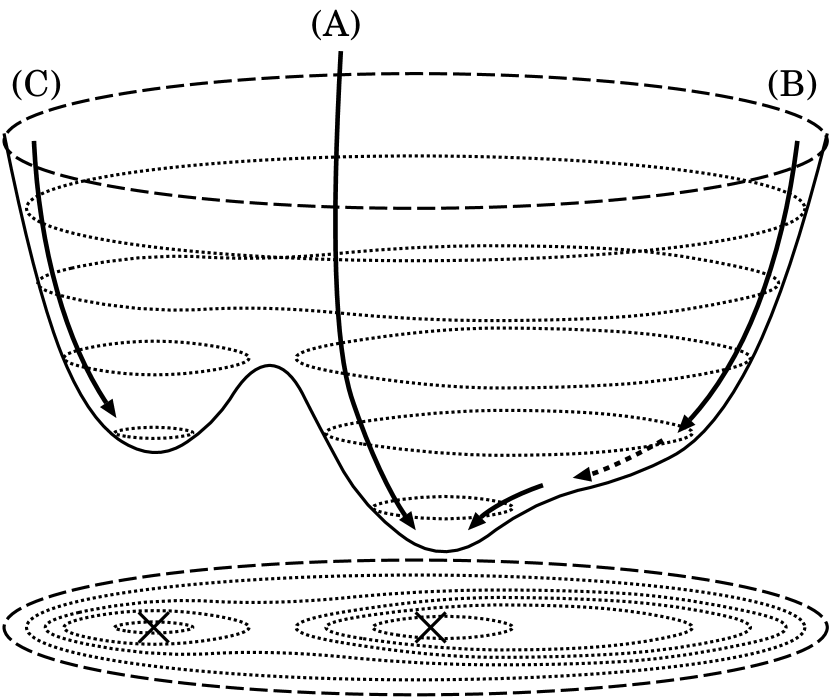
Figure 1: Schematic picture of the energy surface. Two crosses represents minima of the energy surface. Three paths, (A), (B) and (C), show imaginary-time trajectories starting from different initial S-det’s. The dotted arrow of (B) indicates the trajectory (B) passes through a shoulder state.

III.1 Generation and selection of S-det’s

The first step is to prepare a set of S-det’s that span the space necessary for low-lying states with the full long-range correlations. We make use of the imaginary-time method starting from initial configurations which are generated stochastically. The imaginary-time method is often used to obtain self-consistent solutions. Instead, we utilize it for generating many kinds of low-energy collective surfaces. We pick up S-det’s on the way to the self-consistent solutions before reaching minima, and employ them in the configuration mixing calculation.

Figure 1 shows a schematic picture of the imaginary-time calculations starting from different initial configurations. The imaginary-time iteration has a property suitable for generating the basis to calculate the long-range correlations. It quickly removes high-energy components of the wave function in a early stage of the iteration. The S-det is expected to rapidly fall onto a potential energy surface important for low-energy modes of excitation. This is the very property we want, because we should exclude S-det’s which take account of the short-range correlation in the Hamiltonian. Therefore, we simply dispose all the S-det’s generated in the first few hundred iterations of the imaginary-time evolution, then select S-det’s after the rate of energy decrease becomes relatively slow.

A series of S-det’s generated with the imaginary-time calculation starting from an arbitrary initial state eventually converge to a self-consistent solution; either the Hartree-Fock ground state (path (A) and (B) in Fig. 1) or local minima solutions (path (C) in Fig. 1). During the iterations, it sometimes happens that the configuration changes very slowly and the state stays almost unchanged for a long period of the iterations (a part presented by the dotted arrow of path (B)). This is called a shoulder state. Although these shoulder states are not self-consistent solutions, they may play an important role for the low-lying excitation spectra and the ground-state correlation.

We repeat the imaginary-time iteration many times starting from different initial configurations. We construct the initial S-det’s by a stochastic procedure: The single-particle orbitals of the initial S-det are in a Gaussian form whose centers are randomly chosen. After generating large number of imaginary-time trajectories, we may expect that those S-det’s span the complete space for calculation of the long-range correlations.

Figure 2 is an example of the actual imaginary-time calculations for ¹⁶O, showing the energy expectation value, $E(N_{\text{it}})=\langle{\Phi(N_{\text{it}})}|H|{\Phi(N_{\text{it}})}\rangle$, as a function of the iteration number, $N_{\text{it}}$. The path is similar to (B) in Fig. 1, passing through a shoulder state. In $N_{\text{it}}<100$, the energy expectation value decreases very rapidly. From $N_{\text{it}}=200$ to 1500, the energy decreases very slowly, corresponding to a shoulder state. We have found that this shoulder state corresponds to the cluster structure of ¹²C+$\alpha$, which is considered as a dominant component of the first excited state of ¹⁶O in the cluster model studies. The dashed and dash-dotted curves are the energy expectation value after parity projection, $E^{(\pm)}(N_{\text{it}})=\langle{\Phi^{(\pm)}(N_{\text{it}})}|H|{\Phi^{(\pm)}(N_{\text{it}})}\rangle/\langle\Phi^{(\pm)}(N_{\text{it}})|\Phi^{(\pm)}(N_{\text{it}})\rangle$, where $|{\Phi^{(\pm)}(N_{\text{it}})}\rangle=P^{\pm}|{\Phi(N_{\text{it}})}\rangle$.

Figure 2: An example of the imaginary-time evolution in ${}^{16}{\rm O}$ started from a randomly generated S-det. Solid line indicates energy expectation value of the S-det, $|{\Phi(N_{\text{it}})}\rangle$, as a function of iteration number, $N_{\text{it}}$. Snapshots of the density distribution at every 500 iterations are shown. The dashed and the dash-dotted line indicate energy of even and odd parity component of the S-det, respectively. The imaginary-time step of $\Delta\tau=0.001$ $\hbar/$MeV is adopted in the calculation.

III.2 Selection of S-det’s

During the imaginary-time iterations of $N_{\rm total}$ steps, S-det’s for every $N_{\text{s}}$ iterations are taken as candidates of the basis states. Thus, the S-det’s at $N_{\text{it}}^{\text{c}}=N_{\text{s}},2N_{\text{s}},\cdots,k_{\text{n}}N_{\text{s}}$ are nominated first. The number of S-det’s taken from a single path is $k_{\text{n}}=N_{\rm total}/N_{\rm s}$. The typical numbers are $N_{\rm s}=50$ and $N_{\text{total}}=2000$, leading to $k_{\rm n}=40$. However, we cannot include all these S-det’s in the basis set of the configuration mixing calculation, because too many S-det’s lead to a numerical instability caused by the overcompleteness. Thus, we need to reduce their number. Here, we impose two additional constraints on those candidates:

1. $E(N_{\text{it}}^{\text{c}})<E_{\text{HF}}+30$ MeV.

2. Overlap between any pair of selected S-det’s must be less than 0.7 (see below for details).

The condition (a) means that the energy expectation value of each S-det, $E(N_{\text{it}}^{\text{c}})=\langle{\Phi(N_{\text{it}}^{\text{c}})}|H|{\Phi(N_{\text{it}}^{\text{c}})}\rangle$, should not be so large because we are interested in low-lying states and the long-range correlations only. In the present work, we adopt the cut-off energy as 30 MeV above the Hartree-Fock ground-state energy.

The second condition is directly related to the linear independence among the S-det’s. In order to determine whether to include a candidate in the basis set, we examine the overlaps between the new S-det (candidate) and all the S-det’s which have been already included in the basis set. If the maximum of the absolute values of the overlap is less than a certain value, we add the candidate to the set of basis states. Since we make parity and angular momentum projection later, it is desirable to check this condition for projected wave functions. However, it costs too much to achieve angular momentum projection at this stage. Instead, we examine the overlap for different configurations produced by the interchange and the inversion of the Cartesian axes. These transformations correspond to 24 choices of the coordinate system, and are easily realized in the 3D Cartesian coordinate representation. The condition (b) for adding a new S-det $|{\Phi(N_{\text{it}}^{\text{c}})}\rangle$ to the selected basis set $\{|{\Phi_{n}}\rangle;n=1,\cdots,M\}$ is expressed by

$$\frac{|\langle{\Phi(N_{\text{it}}^{\rm c})}|P^{\pm}{\hat{R}}^{i}|{\Phi_{n}}\rangle|}{|\langle{\Phi(N_{\text{it}}^{\rm c})}|P^{\pm}|{\Phi(N_{\text{it}}^{\rm c})}\rangle\langle{\Phi_{n}}|P^{\pm}|{\Phi_{n}}\rangle|^{\frac{1}{2}}}<0.7,$$

$$\quad\quad\quad\mbox{ for }n=1,\cdots,M,$$ (4)

where $\hat{R}^{i},i=1\cdots 24$ are special rotations and inversions corresponding to permutation of the axes $(x,y,z)$.

In practice, the Hartree-Fock state $|{\Phi_{\text{HF}}}\rangle$ is always selected first. Then, we start the examination of constraints (a) and (b) for generated S-det’s $|{\Phi(N_{\text{it}}^{\text{c}})}\rangle$ in the ascending order of the energy expectation value. Here, we employ not the energy expectation values with respect to the S-det, but those with respect to the states projected onto negative parity, $P^{-}|{\Phi(N_{\text{it}}^{\text{c}})}\rangle$. This makes it easier to select exotic deformations which often appear in the negative-parity excited states. For the case in Fig. 2, states at $N_{\text{it}}\approx 2000$ are examined first. Since those around $N_{\text{it}}\approx 500$ also show local minima in the energy surface of negative parity, they are also nominated with high priority.

The number of S-det’s satisfying the criteria (a) and (b) are typically from zero to three in a single trajectory of the imaginary-time evolution. Apparently, larger the number of selected S-det’s, $M$, more difficult it becomes to find the $(M+1)$-th S-det to satisfy the condition (b). In actual calculations, about 100 imaginary-time trajectories will be repeatedly generated to obtain about fifty S-det’s which satisfy these conditions.

IV Parity and angular momentum projection

IV.1 Projection with respect to 3D Euler angles

For each S-det in a set $\{|{\Phi_{n}}\rangle;n=1,2,\cdots,N$ } which are generated and selected in Sec. III. we perform the parity and angular momentum projection. Since we construct wave functions employing the 3D Cartesian coordinate representation without any restrictions on the spatial symmetries, the full three-dimensional angular momentum projection is necessary. The three Euler angles, $(\alpha,\beta,\gamma)$, are abbreviated as $\Omega$. The angular momentum projection operator $P^{J}_{MK}$ is given as usual by

$$P^{J}_{MK}=\frac{2J+1}{8\pi^{2}}\int\!d\Omega D^{J*}_{MK}(\Omega){\hat{R}}(\Omega),$$ (5)

where $D^{J}_{MK}(\Omega)$ is the Wigner’s $D$-function and $\hat{R}(\Omega)$ is the rotation operator.

Quantities necessary for solving a generalized eigenvalue equation in Sec. V are matrix elements of the norm and Hamiltonian kernels. For two S-det’s, $|{\Phi_{n}}\rangle$ and $|{\Phi_{n^{\prime}}}\rangle$, we calculate matrix elements for parity and angular momentum projected wave functions.

$$\left\{\!\!\begin{array}[]{c}N^{J(\pm)}_{nK,n^{\prime}K^{\prime}}\\ H^{J(\pm)}_{nK,n^{\prime}K^{\prime}}\end{array}\!\!\right\} \equiv \langle{\Phi_{n}}|P^{\pm\dagger}P^{J\dagger}_{MK}\left\{\!\!\begin{array}[]{c}1\\ {\hat{H}}\end{array}\!\!\right\}P^{J}_{MK^{\prime}}P^{\pm}|{\Phi_{n^{\prime}}}\rangle=\langle{\Phi_{n}}|\left\{\!\!\begin{array}[]{c}1\\ {\hat{H}}\end{array}\!\!\right\}P^{J}_{KK^{\prime}}P^{\pm}|{\Phi_{n^{\prime}}}\rangle$$ (12)

$$= \frac{2J+1}{16\pi^{2}}\int\!d\Omega D^{J*}_{KK^{\prime}}(\Omega)\times\langle{\Phi_{n}}|e^{-i\alpha{\hat{J}}_{z}}\left\{\!\!\begin{array}[]{c}1\\ {\hat{H}}\end{array}\!\!\right\}(1\pm{\hat{P}})e^{-i\beta{\hat{J}}_{y}}e^{-i\gamma{\hat{J}}_{z}}|{\Phi_{n^{\prime}}}\rangle,$$ (15)

where $K$ and $K^{\prime}$ specifies quantum numbers for body-fixed component of the angular momentum operator. Since the rotation operator commutes with the Hamiltonian, we apply rotations of angles $\beta$ and $\gamma$ to the ket vector $|{\Phi_{n^{\prime}}}\rangle$ and the rotation of $\alpha$ to the bra vector $\langle{\Phi_{n}}|$ in the practical calculations. The parity projection operator is given by $P^{\pm}=(1/2)(1\pm{\hat{P}})$, where ${\hat{P}}$ is the space inversion operator.

The parity transformation and rotation of the S-det, $|{\Phi}\rangle=\det\{|{\phi_{k}}\rangle\}/\sqrt{A!}$, are achieved by the corresponding transformation of their single-particle orbitals, $|{\phi_{k}}\rangle$, $k=1,\cdots,A$. The rotation of finite angle is realized by successive rotations of a small angle. For instance, for a rotation of angle $\alpha$ around $z$-axis,

$$|{\phi_{k}^{\alpha}}\rangle\equiv e^{-i\alpha\hat{j}_{z}}|{\phi_{k}}\rangle=\left(e^{-i\Delta\alpha\hat{j}_{z}}\right)^{N_{\text{div}}}|{\phi_{k}}\rangle,\quad\Delta\alpha=\alpha/N_{\text{div}}.$$ (16)

Each small-angle rotation is performed using the Taylor expansion of the rotation operator;

$$|{\phi^{\alpha+\Delta\alpha}_{k}}\rangle = e^{-i\Delta\alpha\hat{j}_{z}}|{\phi^{\alpha}_{k}}\rangle$$ (17)

$$\approx \sum^{N_{\text{max}}}_{k=0}\frac{(-i\Delta\alpha\hat{j}_{z})^{k}}{k!}|{\phi^{\alpha}_{k}}\rangle,$$

where $N_{\text{max}}=4$ gives an accurate result. We usually employ $\Delta\alpha=2\pi/360$.

The integrand of Eq. (15) is the overlap/Hamiltonian matrix element between two different S-det’s, $e^{-i\alpha\hat{J}_{z}}|{\Phi_{n}}\rangle$ and $(\hat{P})e^{-i\beta\hat{J}_{y}}e^{-i\gamma\hat{J}_{z}}|{\Phi_{n^{\prime}}}\rangle$. These matrix elements are simply expressed in terms of the interstate density matrix defined in Appendix.

IV.2 Numerical details of the projection

We here discuss numerical accuracy of the 3D angular momentum projection. Numerical error in the matrix elements of Eq. (15) may cause a serious trouble when we solve the generalized eigenvalue problem of Eq. (2). For instance, the norm matrix, $N_{nK,n^{\prime}K^{\prime}}^{J\pm}$, should be positive definite, however, in practice, calculated norm matrix suffers from many negative eigenvalues though their absolute values are small.

The finite difference approximation for the angular momentum and the finite-order expansion for the rotation operator in Eq. (17) are good approximation. We have examined the identity of the single-particle orbitals before and after rotating over $2\pi$. The overlap between these two single-particle wave functions is very close to unity, with error less than $10^{-4}$. Therefore, the error in each rotated wave function is relatively small. However, it seems that these numerical errors are accumulated during the 3D integration over Euler angles, $0\leq\alpha<2\pi$, $0\leq\beta<\pi$, and $0\leq\gamma<2\pi$.

The numerical integration is carried out using the trapezoidal rule with the finite-number discretization. Figure 3 shows the norm eigenvalues calculated for $J^{\pi}=3^{-}$ in ¹⁶O. Fifty Slater determinants are generated in the procedure explained in Sec. III, thus the dimension of the norm matrix is 350 ($=7\times 50$ where 7 is the number of different $K$ quantum numbers). The eigenvalues of norm matrix $N^{3(-)}_{nK,n^{\prime}K^{\prime}}$ are plotted in descending order. The left three panels show the eigenvalues when the number of grid points of the angle $\beta$ is varied from 20 to 80 while those for $\alpha$ and $\gamma$ are fixed at 20. For the right panels, we vary the number for $\alpha$ and $\gamma$ from 10 to 40, being fixed at 20 for $\beta$. The norm eigenvalues are converged for $\alpha$ and $\gamma$ if we adopt 15 or more grid points for their discretization. In contrast, the convergence with respect to $\beta$ is rather slow and we still have about 70 negative eigenvalues with 80 grid points. Apparently, it is desirable to have larger number of grid points for the discretization of $\beta$ angle. However, we must make a compromise and sacrifice some accuracy, because the calculation for the Hamiltonian kernels in Eq. (15) are very demanding in the 3D rotation. In the present work, we employ discretization of 15 grid points for $\alpha$ and $\gamma$ and 20 points for $\beta$. Even with this discretization, we need to evaluate 4,500 matrix elements for each pair of the S-det’s.

A price of sacrificing the accuracy is a complication of solving the eigenvalue problem, due to appearance of negative norm. In Sec V, we will explain how to cope with this difficulty.

Figure 3: Eigenvalues of norm matrix for $J^{\pi}=3^{-}$ in ¹⁶O. The horizontal line indicates the sequential number according to the magnitude of the eigenvalues. The top, middle and bottom panels show those of No. 1 to 200, 200 to 320, and 320 to 350, respectively. The norm matrix is calculated with various discretization on Euler angles. In the left panels, $\beta$ is discretized into 20 (squares), 40 (circles), and 80 (triangles) points, while $\alpha$ and $\gamma$ are discretized into 20 points. In the right panels, $\alpha$ and $\gamma$ are discretized into 10 (squares), 20 (circles), and 40 (triangles) points, while $\beta$ is into 20 points.

V Configuration mixing; energy spectra of ¹⁶O

V.1 Zero- and negative-norm problem

Although we collect a set of linearly independent S-det’s in the procedure explained in Sec. III, the linear independence is often lost after the parity and angular momentum projection. This will lead to number of eigenvalues of the norm matrix close to zero. Moreover, the numerical error in the angular momentum projection even produces the negative eigenvalues. In order to solve the eigenvalue equation (2), we must remove states which cause the zero and negative eigenvalues. In this section, we give a possible prescription for this.

For each angular momentum state $J$, we reduce the dimension of the configuration space as follows. We first diagonalize the norm matrix in different $K$ states for each S-det. This is the diagonalization of $(2J+1)\times(2J+1)$ matrix,

$$\sum_{K^{\prime}=-J}^{J}N^{J(\pm)}_{nK,nK^{\prime}}v^{n\nu}_{K^{\prime}}=\lambda_{n\nu}^{J(\pm)}v^{n\nu}_{K}.$$ (18)

Here the eigenstates are labeled by $\nu$. After the $K$-diagonalization, the basis is specified by the label $\nu$, instead of $K$. The collected basis states are denoted as $\{|{\Psi_{n\nu}^{J(\pm)}}\rangle\}_{n,\nu,J}$;

$$|{\Psi_{n\nu}^{J(\pm)}}\rangle_{M}=\sum_{K}v^{n\nu}_{K}P^{J}_{MK}P^{\pm}|{\Phi_{n}}\rangle,\quad M=-J,\cdots,J.$$ (19)

The magnetic quantum number in the laboratory frame, $M$, is a trivial conserved quantity simply giving the $(2J+1)$-fold degeneracy for each state, thus omitted hereafter. At this stage, we exclude states whose eigenvalues $\lambda_{n\nu}^{J(\pm)}$ are smaller than $10^{-2}$. A small eigenvalue will appear when, for example, the S-det is an approximate eigenstate of a specific $K$ quantum number. In the case of $J^{\pi}=3^{-}$ of ¹⁶O, we have 350 configurations constructed from fifty S-det’s, among which about one hundred configurations have $\lambda_{n\nu}^{J(\pm)}$ less than $10^{-2}$ and are discarded.

Although the states in $\{|{\Psi_{n\nu}^{J(\pm)}}\rangle\}_{n,\nu,J}$ are truncated according to the norm eigenvalues, in order to avoid numerical instability, we need to reduce the number furthermore. For this purpose, we consider a following “normalized” norm matrix,

$${\tilde{N}}^{J(\pm)}_{n\nu,n^{\prime}\nu^{\prime}}\equiv\frac{N^{J(\pm)}_{n\nu,n^{\prime}\nu^{\prime}}}{\left(N^{J(\pm)}_{n\nu,n\nu}\right)^{1/2}\left(N^{J(\pm)}_{n^{\prime}\nu^{\prime},n^{\prime}\nu^{\prime}}\right)^{1/2}},$$ (20)

which is constructed so as to make the diagonal elements ${\tilde{N}}^{J(\pm)}_{n\nu n\nu}$ equal to unity. We make a further selection according to the magnitude of eigenvalues of this matrix, $\tilde{\lambda}_{i}$, obtained by solving

$$\sum_{n^{\prime}\nu^{\prime}}{\tilde{N}}^{J(\pm)}_{n\nu,n^{\prime}\nu^{\prime}}u^{i}_{n^{\prime}\nu^{\prime}}=\tilde{\lambda}_{i}u^{i}_{n\nu},$$ (21)

for each parity and angular momentum sector. The existence of small eigenvalue, $\tilde{\lambda}_{i}\ll 1$, indicates a strong overcompleteness of the basis set. We impose the condition on the eigenvalues, that the smallest eigenvalue, $\tilde{\lambda}_{\text{min}}$, must be greater than $10^{-3}$. This is done by the following procedure. First, we calculate eigenvalues of $2\times 2$ matrix of ${\tilde{N}}^{J(\pm)}_{n\nu,n^{\prime}\nu^{\prime}}$ for all possible pairs of $(|{\Psi_{n\nu}^{J(\pm)}}\rangle,|{\Psi_{n^{\prime}\nu^{\prime}}^{J(\pm)}}\rangle)$. If the smaller eigenvalue is less than $10^{-3}$, we remove one of them according to the magnitude of its diagonal element (remove $|{\Psi_{n^{\prime}\nu^{\prime}}}\rangle$ if ${\tilde{N}}^{J(\pm)}_{n^{\prime}\nu^{\prime},n^{\prime}\nu^{\prime}}<{\tilde{N}}^{J(\pm)}_{n\nu,n\nu}$). The number of basis states, $\{|{\Psi_{n\nu}^{J(\pm)}}\rangle\}$ surviving these screenings is now denoted as $N_{\rm sc}$. For the $J^{\pi}=3^{-}$ states of ¹⁶O, $N_{\text{sc}}$ is of order of one hundred. If the $\tilde{\lambda}_{\text{min}}$ of the $N_{\text{sc}}\times N_{\text{sc}}$ matrix, ${\tilde{N}}^{J(\pm)}_{n\nu,n^{\prime}\nu^{\prime}}$, is larger than $10^{-3}$. we can proceed to the configuration mixing calculation to solve Eq. (24). Otherwise, we will further reduce the number of states: We diagonalize the matrix ${\tilde{N}}^{J(\pm)}_{n\nu,n^{\prime}\nu^{\prime}}$ in a space spanned by the basis except for a single state, $|{\Psi_{m\mu}^{J(\pm)}}\rangle$. This is the diagonalization of the $(N_{\rm sc}-1)\times(N_{\rm sc}-1)$ matrix. We do this $N_{\text{sc}}$ times for all possible $|{\Psi_{m\mu}^{J(\pm)}}\rangle$, in order to find the one, $|{\Psi_{m\mu}^{J(\pm)}}\rangle_{\text{ex}}$, for which the minimum eigenvalue of the remaining $(N_{\rm sc}-1)\times(N_{\rm sc}-1)$ matrix becomes the largest. This state, $|{\Psi_{m\mu}^{J(\pm)}}\rangle_{\text{ex}}$, is removed from the basis set. This process is repeated and the number of basis is reduced one by one, until all the eigenvalues, ${\tilde{\lambda}}_{i}$ ($i=1,\cdots,N_{\text{b}}^{J(\pm)}$), becomes larger than $10^{-3}$. In the case of $J^{\pi}=3^{-}$ in ¹⁶O, several dozens of configurations of $|{\Psi_{m\mu}^{3(-)}}\rangle$ are discarded in this screening, so that the final number of the basis states is $N_{\text{b}}^{3(-)}\approx 50$. Note that $N_{\text{b}}^{J(\pm)}$ is the number of states in $\{|{\Psi_{n\nu}^{J(\pm)}}\rangle\}$, thus the number of adopted S-det’s (that of $|{\Phi_{n}}\rangle$) is in general less than $N_{\text{b}}^{J(\pm)}$.

In order to check numerical accuracy and stability, it is convenient to define a “normalized” norm eigenstate corresponding to an eigenvalue $\tilde{\lambda}_{i}$ as

$$|{\Psi^{JM(\pm)}_{i}}\rangle_{M}\equiv\frac{1}{\sqrt{\tilde{\lambda}_{i}}}\sum_{n\nu}\frac{u^{i}_{n\nu}}{\sqrt{N^{J(\pm)}_{n\nu,n\nu}}}\sum_{K}v^{n\nu}_{K}P^{J}_{MK}P^{\pm}|{\Phi_{n}}\rangle.$$ (22)

Using these states as a basis, we calculate the norm and Hamiltonian kernel matrices,

$$\tilde{N}^{J(\pm)}_{ij}\equiv\langle\Psi_{i}^{J(\pm)}|\Psi_{j}^{J(\pm)}\rangle,\quad\quad\tilde{H}^{J(\pm)}_{ij}\equiv\langle{\Psi_{i}^{J(\pm)}}|H|{\Psi_{j}^{J(\pm)}}\rangle,$$ (23)

and solve the generalized eigenvalue equation

$$\sum_{j=1}^{N_{\text{b}}^{J(\pm)}}\left\{{\tilde{H}}^{J(\pm)}_{ij}-E^{J(\pm)}{\tilde{N}}^{J(\pm)}_{ij}\right\}\tilde{g}_{j}^{J(\pm)}=0.$$ (24)

We obtain the energy eigenvalues $E^{J(\pm)}$ and the eigenvectors $\tilde{g}_{i}^{J(\pm)}$.

Figure 4: Energies and norm eigenstates of $J^{\pi}$=$0^{+}$ states (left) and $3^{-}$ states (right) in ${}^{16}{\rm O}$. The top panels show calculated energy $E^{J(\pm)}$ of Eq. (24) as a function of dimension of the adopted model space. The middle and bottom panels show $\tilde{\lambda}_{i}$ and $\tilde{E}_{i}^{J(\pm)}=\tilde{H}_{ii}^{J(\pm)}$, respectively. See text for details.

V.2 Quality of solutions

In this section, we examine quality of solutions obtained by diagonalizing Eq. (24) and how “complete” the selected basis is. Let us emphasize again that we do not intend to obtain the exact eigenstates of a given Hamiltonian. The exact ground state of a Hamiltonian with the zero-range interaction such as Eq. (3) perhaps leads to an unphysical solution. Instead, we aim to take into account correlations of its long-range part only. Therefore, we examine whether the method can produce convergent results for low-lying states.

Let us suppose that we have selected $N_{\text{b}}^{J(\pm)}$ basis states for specific parity and angular momentum, $(J,M,\pm)$. We solve Eq. (21) to obtain eigenvalues, $\tilde{\lambda}_{i}$, and vectors, $u_{n\nu}^{i}$, then construct the norm eigenstates of Eq. (22), $|{\Psi_{i}^{J(\pm)}}\rangle$. First, the states $\{|{\Psi_{i}^{J(\pm)}}\rangle\}$ are sorted according to the magnitude of their norm eigenvalues, $\tilde{\lambda}_{i}$. Thus, the eigenstates are arranged in sequence of $\tilde{\lambda}_{1}>\tilde{\lambda}_{2}>\cdots>\tilde{\lambda}_{N_{\text{b}}}$. The middle and bottom panels in Fig. 4 show distributions of $\tilde{\lambda}_{i}$ and the diagonal elements of the Hamiltonian, $\tilde{E}_{i}^{J(\pm)}=\tilde{H}_{ii}^{J(\pm)}$, respectively, for $J^{\pi}=0^{+}$ (left) and $3^{-}$ states (right) in ¹⁶O. In this calculation, there are 19 basis states for $J^{\pi}=0^{+}$ and 53 for $J^{\pi}=3^{-}$ for which all the norm eigenvalues are larger than $10^{-3}$. The $\tilde{\lambda}_{i}$ decrease linearly in the logarithmic scale. An interesting thing is the fact that the energy expectation values, $\tilde{E}_{i}^{J(\pm)}$, are closely correlated with the norm eigenvalues $\tilde{\lambda}_{i}$. The energies $\tilde{E}_{i}^{J(\pm)}$ roughly show a monotonic increase with $i$, as $\tilde{\lambda}_{i}$ decrease. This may justify the screening process to discard states with small norm eigenvalues, because those states possess large energy expectation values and are expected not to play a significant role for low-energy excitations.

The top panels in Fig. 4 show resultant energy eigenvalues, $E^{J(\pm)}$, obtained by the diagonalization of Eq. (24). The horizontal axis indicates the number of basis states included in the calculation, which is increased one by one from left to right; $\{|{\Psi_{1}^{J(\pm)}}\rangle\}$, $\{|{\Psi_{1}^{J(\pm)}}\rangle,|{\Psi_{2}^{J(\pm)}}\rangle\}$, $\cdots$, $\{|{\Psi_{1}^{J(\pm)}}\rangle,\cdots,|{\Psi_{N_{\text{b}}}^{J(\pm)}}\rangle\}$. Calculated spectra for $J^{\pi}=0^{+}$ and $3^{-}$ states in ¹⁶O are shown in the left and right panels, respectively. As is seen in the figure, low-energy spectra become almost invariant with respect to the inclusion of new basis states. In other words, energies of the ground and low-lying states are insensitive to the inclusion of states with small norm eigenvalues. These convergent behaviors suggest that the long-range correlations for low-lying states are taken into account in the calculation.

To further examine the completeness of the basis states, we check the identity of results produced with different sets of basis states (initially generated with different random numbers). If our prescription provides a complete set of basis for the long-range correlations of the Hamiltonian, the energy spectra should not depend on the initial S-det’s from which the imaginary-time iteration started. In Fig. 5, excitation energies in the ¹⁶O nucleus calculated with four different sets of S-det’s are compared. In these four independent calculations, different seeds for the random number were used in preparing the initial S-det’s. The energies of the lowest and the next lowest states for each parity and angular momentum $(J^{\pi})$ coincide to each other in reasonable accuracy. For example, negative-parity excitations of $1^{-}$, $2^{-}$, and $3^{-}$ states appear below 15 MeV, and there are no other states in this energy region. The results become less reliable for higher states in each $J^{\pi}$ sector. The second $0^{+}$ state (first excited $0^{+}$) appears around $15\sim 17$ MeV in all calculations. However, excitation energy of the third (second excited) $0^{+}$ state in the bottom-left panel is notably higher than the other three.

Figure 5: Excitation energies of ¹⁶O. Symbols at the bottom of each panel indicate the quantum numbers, $J^{\pi}$. Results of calculations employing four different sets of Slater determinants are displayed.

The excitation energy of the second $0^{+}$ state is much higher than the experimental value (6.05 MeV). The three negative-parity excited states with $J^{\pi}=3^{-}$, $1^{-}$, and $2^{-}$, are observed at 6.13, 7.12, and 8.87 MeV, respectively. Since the BKN interaction adopted in the present work, which does not contain the spin-orbit interaction, is too simple to give a quantitative description of nuclear structure, one should not seriously take these discrepancies between the calculation and the experiment.

We also perform the same examination for other nuclei discussed below, ¹²C and ²⁰Ne. The final number of basis states $N_{\text{b}}^{J(\pm)}$ and behavior of the convergence is similar to those of ¹⁶O. The comparison of results among sets of basis generated with different random numbers may provide a useful information about reliability of calculations. From these analysis, we may judge how many eigenstates in each $J^{\pi}$ sector can be trusted.

Before finishing this section, let us comment on the cut-off value of the norm eigenvalues. In the bottom panels of Fig. 4, the energy expectation values become somewhat scattered as the norm eigenvalues, $\tilde{\lambda}_{i}$, approach to $10^{-3}$. This may be an indication of the numerical instability. In fact, if we include basis functions with $\tilde{\lambda}_{i}<10^{-3}$, the configuration mixing leads to unphysical solutions. For instance, if we set a cut-off of $\tilde{\lambda}_{i}>10^{-4}$, the ground state becomes completely different from the Hartree-Fock state and its energy is unreasonably lowered by the diagonalization of the Hamiltonian. It is most likely that this problem originates from the numerical error in evaluating the matrix elements, especially in the angular momentum projection.

VI Energy spectra of ¹²C and ²⁰Ne

Figure 6: Calculated and experimental excitation energy spectra of ${}^{20}{\rm Ne}$. Symbols at the bottom of each panel indicate the quantum numbers, $J^{\pi}$.

Figure 7: The same as Fig. 6 but for ${}^{12}{\rm C}$.

The BKN interaction of Eq. (3) is adopted for testing our new method. As we have mentioned before, one should not expect a quantitative description of the low-lying spectra. However, the present calculation gives a reasonable description for some excited states of light nuclei, especially for those composed of the $LS$-closed clusters. In this section, we present calculated energy spectra of ²⁰Ne and ¹²C nuclei. In these nuclei, there appear the $LS$-closed clusters in the ground and excited states ($\alpha$+¹⁶O for ²⁰Ne and 3$\alpha$ for ¹²C). In this paper, we restrict our discussion on the energy spectra in these $N=Z$ even-even nuclei. A detailed discussion on the structure of excited states including information on the transition matrix elements will be given in our next work employing a realistic Skyrme interaction.

Figure 6 shows calculated energy spectra (left panel) and those in measurement (right) in ²⁰Ne. It has been well-known that the $K^{\pi}=0^{+}$ ground state band and the $K^{\pi}=0^{-}$ negative-parity band starting with $1^{-}$ state at 5.785 MeV constitute a kind of inversion doublet band of the $\alpha$-¹⁶O cluster structure. This inversion doublet bands are reasonably described in our calculation. In the measurement, the lowest negative parity band is the $K^{\pi}=2^{-}$ band at 4.968 MeV. In our calculation, it is around 9 MeV, reflecting the importance of the spin-orbit splitting of $p$ and $d$ orbitals for this excitation.

We next discuss results for ¹²C whose spectra are shown in Fig. 7. Again, the calculation (left panel) is compared with measured spectra (right). The calculation produce the ground state rotational band, but its moment of inertia is significantly larger than the observed values. In the negative parity, our calculation produces $3^{-}$ state in the lowest energy, also $1^{-}$ and $2^{-}$ states at low excitation energies. These are qualitatively in agreement with experiments. In the positive parity excited states, the calculation indicates two $0^{+}$ states around 10 and 12 MeV. These may correspond to the measured states around 8 and 10 MeV.

In Refs. PPHF , we have reported the variation after parity projection calculation employing the BKN interaction. The angular momentum projection after variation is achieved in the calculation employing Skyrme force PPSHF ; PhD:Ohta ; PPSHF-P . A part of results presented in this section coincide fairly well with these variation after parity projection calculations. This suggests that the variation after parity projection gives a dominant correlation for a certain class of states (with clustering) in ¹²C and ²⁰Ne.

VII Summary

In this paper, we report our attempt to develop a new computational method to include all the long-range correlations beyond the mean-field approximation. We aim at a systematic description of the ground and low-lying excited states using a mean-field Hamiltonian, without assuming their structure a priori.

First, we stochastically generate many Slater determinants. The single-particle orbitals are expressed on the three-dimensional Cartesian grid representation. In order to remove high-energy components in those states, we use the imaginary-time iteration method. The imaginary-time evolution produces many trajectories important for low-energy modes of excitation. We select some of these states to keep the linear independence. We then project them on good parity and angular momentum, and perform configuration mixing calculation. The BKN interaction is utilized to examine feasibility and difficulty of the method. We have found that there is a numerical difficulty to achieve the configuration mixing calculation. The eigenvalues of the norm matrix can be close to zero, when the selected states are overcomplete. In the practical calculations, a small numerical error in the angular momentum projection results in the occurrence of negative eigenvalues of the norm matrix. We eliminate states responsible for these zero and negative eigenvalues before solving the generalized eigenvalue problem.

We show calculated results for some light $4N$ nuclei, ¹²C, ¹⁶O, and ²⁰Ne. In these nuclei, appearances of various cluster states are known in excited states. Our calculation provides reasonable excitation energies for $\alpha+^{16}$O states of ²⁰Ne and $3\alpha$ states of ¹²C for which the spin-orbit interaction, which is not included in the BKN force, does not play an important role.

The results calculated with different sets of random numbers are approximately identical to each other. However, the discrepancy becomes more evident for states at higher energies. In the present level of accuracy, we may predict the lowest and possibly the second lowest states in each parity and angular momentum sector. Improvement in numerical accuracy, especially in the three-dimensional angular momentum projection, is desired for future work with more realistic interactions.

*

Appendix A Matrix elements between non-orthogonal Slater determinants

In this appendix, we present useful expressions for calculating matrix elements such as the integrand of Eq. (15). In general, we discuss transition amplitude of an operator $\hat{O}$ between two different S-det’s, $\langle{\Phi}|\hat{O}|{\Psi}\rangle$. The S-det’s are expressed in terms of orthonormal single-particle orbitals, $|{\Phi}\rangle=\det\{|{\phi_{i}(j)}\rangle\}/\sqrt{A!}$ and $|{\Psi}\rangle=\det\{|{\psi_{i}(j)}\rangle\}/\sqrt{A!}$, with $\langle\phi_{i}|\phi_{j}\rangle=\langle\psi_{i}|\psi_{j}\rangle=\delta_{ij}$. Here, we assume $|{\Phi}\rangle$ and $|{\Psi}\rangle$ are not orthogonal to each other. To calculate these matrix elements, it is convenient to define following orbitals,

$$|{\tilde{\psi}_{i}}\rangle=\sum_{j}|{\psi_{j}}\rangle(B^{-1})_{ji}$$ (25)

where the matrix $B$ is defined by $B_{ij}=\langle\phi_{i}|\psi_{j}\rangle$. The overlap matrix element is given by the determinant of $B$, $\langle\Phi|\Psi\rangle=\det B$. It can be easily confirmed that $|{\tilde{\psi}_{i}}\rangle$ are bi-orthogonal to $|{\phi_{j}}\rangle$, having

$$\langle\phi_{i}|\tilde{\psi}_{j}\rangle=\delta_{ij}.$$ (26)

We also note that the S-det constructed from $|{\tilde{\psi}_{i}}\rangle$ is proportional to $|{\Psi}\rangle$,

$$|{\tilde{\Psi}}\rangle\equiv\frac{1}{\sqrt{A!}}\det\left\{\tilde{\psi}_{i}(j)\right\}=\frac{|{\Psi}\rangle}{\langle\Phi|\Psi\rangle}.$$ (27)

Since the S-det $|{\Psi}\rangle$ is now represented by single-particle orbitals $|{\tilde{\psi}_{i}}\rangle$ which have a bi-orthogonal property (26), the matrix elements $\langle{\Phi}|\hat{O}|{\Psi}\rangle$ can be expressed in a familiar form very similar to that of the expectation value, $\langle{\Phi}|\hat{O}|{\Phi}\rangle$. Suppose that, the expectation value of the operator $\hat{O}$, $\langle\Phi|\hat{O}|\Phi\rangle$, is expressed as a functional of the density matrix, $\rho_{ij}(\Phi)=\langle{\Phi}|c_{j}^{\dagger}c_{i}|{\Phi}\rangle$,

$$O[\rho(\Phi)]=\langle{\Phi}|\hat{O}|{\Phi}\rangle.$$ (28)

Then, the matrix element between $|{\Phi}\rangle$ and $|{\Psi}\rangle$ is expressed as

$$\langle{\Phi}|\hat{O}|{\Psi}\rangle=\langle{\Phi}|\hat{O}|{\tilde{\Psi}}\rangle\langle\Phi|\Psi\rangle=O[\tilde{\rho}(\Phi\Psi)]\langle\Phi|\Psi\rangle,$$ (29)

where the interstate density $\tilde{\rho}(\Phi\Psi)$ is defined by

$$\tilde{\rho}_{ij}(\Phi\Psi)=\langle{\Phi}|c_{j}^{\dagger}c_{i}|{\tilde{\Psi}}\rangle.$$ (30)

Therefore, the matrix element between two S-det’s, $\langle{\Phi}|\hat{O}|{\Psi}\rangle$, is given by $O[\rho]\times\det B$, where the density matrix $\rho$ is replaced by the interstate density matrix (30).

References

- (1) B. S. Pudliner, V. R. Pandharipande, J. Carlson, and R. B. Wiringa, Phys. Rev. Lett. 74, 4396 (1995).
- (2) B. S. Pudliner, V. R. Pandharipande, J. Carlson, S. C. Pieper, and R. B. Wiringa, Phys. Rev. C 56, 1720 (1997).
- (3) R. B. Wiringa, S. C. Pieper, J. Carlson, and V. R. Pandharipande, Phys. Rev. C 62, 014001 (2000).
- (4) S. C. Pieper, V. R. Pandharipande, R. B. Wiringa, and J. Carlson, Phys. Rev. C 64, 014001 (2001).
- (5) S. C. Pieper, K. Varga and R. B. Wiringa, Phys. Rev. C 66, 044310 (2002).
- (6) P. Navrátil, J. P. Vary, and B. R. Barrett, Phys. Rev. Lett. 84, 5728 (2000); Phys. Rev. C 62, 054311 (2000).
- (7) P. Ring and P. Schuck, The Nuclear Many-Body Problem (Springer-Verlag, Berlin, 1980).
- (8) D. Vautherin and D. M. Brink, Phys. Rev. C 5, 626 (1972).
- (9) D. Vautherin, Phys. Rev. C 7, 296 (1973).
- (10) J. Dechargé and D. Gogny, Phys. Rev. C 21, 1568 (1980).
- (11) J. D. Walecka, Ann. Phys. 83, 491 (1974).
- (12) M. G. Mayer and J. H. D. Jensen, Elementary Theory of Nuclear Shell Structure, (Wiley, New York, 1955). Nuclear Shell Theory, (Academic Press, New York, 1963).
- (13) A. de-Shalit and I. Talmi, Nuclear Shell Theory (Academic Press, New York, 1963).
- (14) K. Ikeda et al., Prog. Theor. Phys. Suppl. 68 (1980).
- (15) A. Ono, H. Horiuchi, T. Maruyama and A. Ohnishi, Prog. Theor. Phys. 87, 1185 (1992).
- (16) Y. Kanada-En’yo and H. Horiuchi, Prog. Theor. Phys. Suppl. 142, 205 (2001).
- (17) Y. Kanada-En’yo, Phys. Rev. Lett 81, 5291 (1998).
- (18) H. Ohta, K. Yabana, and T. Nakatsukasa, Phys. Rev. C 70, 014301 (2004).
- (19) D. L. Hill and J. A. Wheeler, Phys. Rev. 89, 1102 (1953).
- (20) T. Otsuka, M. Honma, T. Mizusaki, N. Shimizu and Y. Utsuno, Prog. Part. Nucl. Phys. 47 319 (2001).
- (21) P. Bonche, S. Koonin, and J. W. Negele, Phys. Rev. C 13, 1226 (1976).
- (22) S. Takami, K. Yabana, and K. Ikeda, Prog. Theor. Phys. 96, 407 (1996).
- (23) H. Ohta, Ph.D. thesis, University of Tsukuba, 2005
- (24) H. Ohta, T. Nakatsukasa, and K. Yabana, Eur. Phys. J. A 25 s01, 549 (2005); J. Phys. Conf. Ser. 20, 211 (2005).