Collective modes in relativistic npe matter at finite temperature

Abstract

Isospin and density waves in neutral neutron-proton-electron (npe) matter are studied within a relativistic mean-field hadron model at finite temperature with the inclusion of the electromagnetic field. The dispersion relation is calculated and the collective modes are obtained. The unstable modes are discussed and the spinodals, which separate the stable from the unstable regions, are shown for different values of the momentum transfer at various temperatures. The critical temperatures are compared with the ones obtained in a system without electrons. The largest critical temperature, 12.39 MeV, occurs for a proton fraction $y_{p}=0.47$. For $y_{p}=0.3$ we get $T_{cr}$=5 MeV and for $y_{p}>0.495$ $T_{cr}\lesssim 8$ MeV. It is shown that at finite temperature the distillation effect in asymmetric matter is not so efficient and that electron effects are particularly important for small momentum transfers.

PACS number(s): 21.60.-n,21.60.Ev,21.65.+f,24.10.Jv,71.10.Ay

I Introduction

In order to describe compact-star matter at low densities, besides protons and neutrons, the electrons (and possibly neutrinos if they are trapped) must be introduced. Electrons neutralize the proton charge and thus suppress the diverging Coulomb contribution to the energy. This composite matter is expected to undergo phase transitions associated to the nuclear liquid-gas phase transition but strongly modified by the Coulomb interaction and the presence of electrons. Phase transitions in asymmetric matter are related with the instability regions limited by the spinodal sections instabilities1 ; previous . These very same instabilities are responsible for nucleation processes gotas and the possible existence of a non-homogeneous phase. At low nuclear matter densities, which are the densities of relevance in the present work, a competition between the long-range Coulomb repulsion and short-range nuclear attraction can lead to the formation of matter known as nuclear pasta pasta . The competition of these two forces, normally acting on different scales, is called frustration. This novel state of matter, the nuclear pasta, can appear in different structures and its properties have important consequences in the crust of neutron stars and in the core-collapse of supernova horo2 ; wata04 ; maru ; hpbp . Not only the equation of state of stellar matter has to be understood, but also the neutrino mean free path in the medium has to be well described. In fact, neutrino interactions are crucial in the dynamics of the core-collapse supernovae because they carry most of the energy away. It has been shown that the neutrino opacity is affected by nucleon-nucleon interactions due to coherent scattering off density fluctuations sawyer . Both single particle and collective contribution have to be taken into account. In rbp it was shown that coherent neutrino scattering from non-uniform hadron-quark matter or hadron matter with and without kaon condensed phase would greatly reduce the neutrino mean-free path. A similar effect at low densities could allow enough energy transfer in order to revive the supernova shock. Recent semiclassical simulations of the linear response of nuclear non-homogenous matter at low densities, the so called nuclear pasta, to neutrinos in hpbp ; horo2 have shown that coherence effects reduce the mean free path of neutrinos. In these simulations electrons are not modeled explicitly, but their effect is included through a modified Coulomb interaction between the protons through a screening length. Neutrinos will loose energy by exciting collective nuclear modes or plasmon modes. However in previous1 it has been shown that the behavior of the electrons depends on the wavelength of the perturbation. In ksg low energy nuclear collective excitations of Wigner-Seitz cells containing nuclear clusters immersed in a gas of neutrons have been obtained. In that paper, the electron motion was not included. Including the electron contribution will likely affect the results for large clusters.

In previous1 we have investigated the influence of the electromagnetic interaction and the presence of electrons on the unstable modes of nuclear matter and compared the dynamical instability region with the thermodynamical one. This investigation was performed in the framework of a relativistic mean field hadronic model within the Vlasov formalism npp91 ; npp93 ; previous . In particular, in previous1 , it has been studied the role of isospin and the modification of the distillation phenomenon due to the presence of the Coulomb field and electrons. These calculations were performed at $T=0$ MeV.

In the present work the effect of dynamical instabilities including the Coulomb field are investigated at finite $T$. Understanding the mixed phase of neutral matter at finite temperature is important to determine the behavior of neutrinos emitted in a supernova explosion.

II The Vlasov equation formalism

We consider a system of baryons, with mass $M$ interacting with and through a isoscalar-scalar field $\phi$ with mass $m_{s}$, a isoscalar-vector field $V^{\mu}$ with mass $m_{v}$ and an isovector-vector field $\mathbf{b}^{\mu}$ with mass $m_{\rho}$. We also include a system of electrons with mass $m_{e}$. Protons and electrons interact through the electromagnetic field $A^{\mu}$. The lagrangian density reads:

$$\mathcal{L}=\sum_{i=p,n}\mathcal{L}_{i}+\mathcal{L}_{e}\mathcal{\,+L}_{{\sigma}}\mathcal{+L}_{{\omega}}\mathcal{+L}_{{\rho}}\mathcal{+L}_{A},$$ (1)

where the nucleon Lagrangian reads

$$\mathcal{L}_{i}=\bar{\psi}_{i}\left[\gamma_{\mu}iD^{\mu}-M^{*}\right]\psi_{i},$$ (2)

with

$$iD^{\mu} = i\partial^{\mu}-g_{v}V^{\mu}-\frac{g_{\rho}}{2}{\vec{\tau}}\cdot\vec{b}^{\mu}-e\frac{1+\tau_{3}}{2}A^{\mu},$$ (3)

$$M^{*} = M-g_{s}\phi,$$ (4)

and the electron Lagrangian is given by

$$\mathcal{L}_{e}=\bar{\psi}_{e}\left[\gamma_{\mu}\left(i\partial^{\mu}+eA^{\mu}\right)-m_{e}\right]\psi_{e}.$$ (5)

The isoscalar part is associated with the scalar sigma ($\sigma$) field, $\phi$, and the vector omega ($\omega$) field, $V_{\mu}$, while the isospin dependence is coming from the isovector vector rho ($\rho$) field, $b_{\mu}^{i}$ (where $\mu$ is the 4 dimensional space-time indices and $i$ the 3D isospin direction indices). The associated Lagrangians are

$$\mathcal{L}_{{\sigma}} = +\frac{1}{2}\left(\partial_{\mu}\phi\partial^{\mu}\phi-m_{s}^{2}\phi^{2}-\frac{1}{3}\kappa\phi^{3}-\frac{1}{12}\lambda\phi^{4}\right)$$

$$\mathcal{L}_{{\omega}} = -\frac{1}{4}\Omega_{\mu\nu}\Omega^{\mu\nu}+\frac{1}{2}m_{v}^{2}V_{\mu}V^{\mu}$$

$$\mathcal{L}_{{\rho}} = -\frac{1}{4}\vec{B}_{\mu\nu}\cdot\vec{B}^{\mu\nu}+\frac{1}{2}m_{\rho}^{2}\vec{b}_{\mu}\cdot\vec{b}^{\mu}$$

$$\mathcal{L}_{A} = -\frac{1}{4}F_{\mu\nu}F^{\mu\nu}$$

where $\Omega_{\mu\nu}=\partial_{\mu}V_{\nu}-\partial_{\nu}V_{\mu}$ , $\vec{B}_{\mu\nu}=\partial_{\mu}\vec{b}_{\nu}-\partial_{\nu}\vec{b}_{\mu}-g_{\rho}(\vec{b}_{\mu}\times\vec{b}_{\nu})$ and $F_{\mu\nu}=\partial_{\mu}A_{\nu}-\partial_{\nu}A_{\mu}$. The model comprises the following parameters: three coupling constants $g_{s}$, $g_{v}$ and $g_{\rho}$ of the mesons to the nucleons, the nucleon mass $M$, the electron mass $m_{e}$, the masses of the mesons $m_{s}$, $m_{v}$, $m_{\rho}$, the electromagnetic coupling constant $e=\sqrt{4\pi/137}$ and the self-interacting coupling constants $\kappa$ and $\lambda$. We have used the set of constants identified as NL3 taken from nl3 . For this case, the saturation density that we refer as $\rho_{0}$ is 0.148 fm^-3. In the above lagrangian density $\vec{\tau}$ is the isospin operator.

Denoting by

$$f({\bf r},{\bf p},t)_{\pm}=\mbox{diag}(f_{p\pm},\,f_{n\pm},\,f_{e\pm})$$

the distribution functions of particles (+) at position $\mathbf{r}$, instant $t$ and momentum $\mathbf{p}$ and of antiparticles (-) at position $\mathbf{r}$, instant $t$ and momentum $-\mathbf{p}$ and the corresponding one-body hamiltonian by

$$h_{\pm}=\mbox{diag}\left(h_{p\pm},h_{n\pm},h_{e\pm}\right)$$ (6)

where

$$h_{i\pm}=\pm\sqrt{({\bf p}-{\boldsymbol{\cal V}_{i}})^{2}+{M^{*}}_{i}^{2}}+{\cal V}_{0i}.$$

For protons and neutrons, $i=p,n$, we have

$${\cal V}_{0i}=g_{v}V_{0}+\frac{g_{\rho}}{2}\,\tau_{i}b_{0}+e\,A_{0}\frac{1+\tau_{i}}{2},$$

$${\boldsymbol{{\cal V}_{i}}}=g_{v}{\mathbf{V}}+\frac{g_{\rho}}{2}\,\tau_{i}{\mathbf{b}}+e\,{\mathbf{A}}\frac{1+\tau_{i}}{2},$$

$$M^{*}_{p}=M^{*}_{n}=M^{*}=M-g_{s}\phi,$$

$\tau_{i}=1$ (protons) or -1 (neutrons), and for electrons, $i=e$, we have

$${\cal V}_{0e}=-e{A}_{0},\,\,\,{\boldsymbol{{\cal V}_{e}}}=-e\,{\mathbf{A}},\,\,\,M^{*}_{e}=m_{e}.$$

The time evolution of the distribution functions is described by the Vlasov equation

$$\frac{\partial f_{i\pm}}{\partial t}+\{f_{i\pm},h_{i\pm}\}=0,\qquad\;i=p,\,n,\,e,$$ (7)

where $\{,\}$ denote the Poisson brackets. From Hamilton’s equations we derive the equations describing the time evolution of the fields $\phi$, $V^{\mu}$, $A^{\mu}$ and the third component of the $\rho$-field $b_{3}^{\mu}=(b_{0},\mathbf{b})$, which are given in the Appendix A.

The state which minimizes the energy of asymmetric npe matter is characterized by the distribution functions

$$f_{0i\pm}=\frac{1}{1+e^{(\epsilon\mp\nu_{i})/T}}\quad i=p,n$$ (8)

with $\epsilon=\sqrt{p^{2}+{M^{*}}^{2}}$,

$$\nu_{i}=\mu_{i}-g_{v}V_{0}-\frac{g_{\rho}}{2}\,\tau_{i}b_{0}-e\,A_{0}\frac{1+\tau_{i}}{2},$$ (9)

and

$$f_{0e\pm}=\frac{1}{1+e^{(\epsilon_{0e}\mp\mu_{e})/T}}$$ (10)

with $\epsilon_{0e}=\sqrt{p^{2}+m_{e}^{2}},$ and by the constant mesonic fields which obey the following equations

$$m_{s}^{2}\phi_{0}+\frac{\kappa}{2}\phi_{0}^{2}+\frac{\lambda}{6}\phi_{0}^{3}=g_{s}\rho_{s}^{(0)}$$

$$m_{v}^{2}\,V_{0}^{(0)}\,=\,g_{v}j_{0}^{(0)},$$

$$m_{\rho}^{2}\,b_{0}^{(0)}\,=\,\frac{g_{\rho}}{2}j_{3,0}^{(0)}\;,$$

$$V^{(0)}_{i}\,=b_{i}^{(0)}\,=\,A_{0}^{(0)}\,=\,A_{i}^{(0)}\,=\,0.$$

Collective modes in the present approach correspond to small oscillations around the equilibrium state. These small deviations are described by the linearized equations of motion and, therefore, collective modes are given as solutions of those equations. To construct them, let us define:

$$f_{i\pm}\,=\,f_{0i\pm}+\delta f_{i\pm}\;,$$

$$\phi\,=\,\phi_{0}+\delta\phi\;,$$

$$V_{0}\,=\,V_{0}^{(0)}+\delta V_{0}\;,\;\;\;V_{i}\,=\,\delta V_{i}\;,$$

$$b_{0}\,=\,b_{0}^{(0)}+\delta b_{0}\;,\;\;\;b_{i}\,=\,\delta b_{i}\;,$$

$$A_{0}\,=\,\delta A_{0}\;,\;\;\;A_{i}\,=\,\delta A_{i}.$$ (11)

As in npp91 ; previous ; instabilities2 we express the fluctuations of the distribution functions in terms of the generating functions

$$S_{\pm}({\mathbf{r}},{\mathbf{p}},t)=\mbox{diag}\left(S_{p\pm},\,S_{n\pm},\,S_{e\pm}\right),$$

such that

$$\delta f_{\pm}=\{S_{\pm},f_{0\pm}\}=\{S_{\pm},p^{2}\}\frac{df_{0\pm}}{dp^{2}}.$$

In terms of the generating functions, the linearized Vlasov equations for $\delta f_{i\pm}$

$$\frac{d\delta f_{i\pm}}{dt}+\{\delta f_{i\pm},h_{0i\pm}\}+\{f_{0i\pm},\delta h_{i\pm}\}=0$$

are equivalent to the following time evolution equations

$$\frac{\partial S_{e\pm}}{\partial t} + \{S_{e\pm},h_{0e\pm}\}=\delta h_{e\pm}=-e\left[\delta{A}_{0}\mp\frac{{\bf p}\cdot\delta{\mathbf{A}}}{\epsilon_{0e}}\right],$$

$$\frac{\partial S_{i\pm}}{\partial t}+\{S_{i\pm},h_{0i\pm}\}=\delta h_{i\pm}=\mp\frac{g_{s}\,M^{*}}{\epsilon}\delta\phi+\delta{\cal V}_{0i}\mp\frac{{\bf p}\cdot\delta\boldsymbol{\cal V}_{i}}{\epsilon},$$ (12)

$i=p,n$, where

$$\delta{\cal V}_{0i}=g_{v}\delta V_{0}+\tau_{i}\frac{g_{\rho}}{2}\,\delta b_{0}+e\,\frac{1+\tau_{i}}{2}\,\delta A_{0},$$

$$\delta\boldsymbol{\cal V}_{i}=g_{v}\delta{\mathbf{V}}+\tau_{i}\frac{g_{\rho}}{2}\,\delta{\mathbf{b}}+e\,\frac{1+\tau_{i}}{2}\,\delta{\mathbf{A}},$$

with $h_{0i\pm}\,=\pm\epsilon+{\cal V}^{(0)}_{0i}$, $i=p,n$ and $h_{0e\pm}\,=\pm\epsilon_{0e}$ . The linearized equations of the fields are shown in the Appendix B.

Of particular interest on account of their physical relevance are the longitudinal modes, with momentum ${\bf k}$ and frequency $\omega$, described by the ansatz

$$\left(\begin{array}[]{c}S_{j\pm}({\bf r},{\bf p},t)\\ \delta\phi\\ \delta B_{0}\\ \delta B_{i}\end{array}\right)=\left(\begin{array}[]{c}{\cal S}_{\omega\pm}^{j}(p,{\rm cos}\theta)\\ \delta\phi_{\omega}\\ \delta B_{\omega}^{0}\\ \delta B_{\omega}^{i}\end{array}\right){\rm e}^{i(\omega t-{\bf k}\cdot{\bf r})}\;,$$

where $j=e,\,p,\,n$, $B=V,\,b,A$ represents the vector fields and $\theta$ is the angle between ${\bf p}$ and ${\bf k}$. For these modes, we get $\delta V_{\omega}^{x}=\delta V_{\omega}^{y}=0\,$, $\delta b_{\omega}^{x}=\delta b_{\omega}^{y}=0\,$ and $\delta A_{\omega}^{x}=\delta A_{\omega}^{y}=0\,$. Calling $\delta V_{\omega}^{z}=\delta V_{\omega}$, $\delta b_{\omega}^{z}=\delta b_{\omega}$ and $\delta A_{\omega}^{z}=\delta A_{\omega}$, we will have

$$\delta{\cal V}_{i,z}=\delta{\cal V}_{\omega}^{i}{\rm e}^{i(\omega t-{\bf k}\cdot{\bf r})},\qquad\delta{\cal V}_{0i}=\delta{\cal V}_{\omega}^{0i}{\rm e}^{i(\omega t-{\bf k}\cdot{\bf r})},$$

and the equations of motion become

$$i(\omega\mp\frac{kp\cos\theta}{\epsilon_{0e}}){\cal S}_{\omega\pm}^{e}\,=\,-e\left[\delta{A}_{\omega}^{0}\mp\frac{p\cos\theta}{\epsilon_{0e}}\delta{A}_{\omega}\right]\;,$$ (13)

$$i\left(\omega\mp\frac{kp\cos\theta}{\epsilon}\right){\cal S}_{\omega\pm}^{i}\,=\,\mp g_{s}\frac{M^{*}}{\epsilon}\delta\phi_{\omega}\mp\frac{p\cos\theta}{\epsilon}\delta{\cal V}_{\omega}^{i}+\delta{\cal V}_{\omega}^{0i}$$ (14)

$$\left(\omega^{2}-k^{2}-m^{2}_{s,eff}\right)\delta\phi_{\omega}\,=\,4ig_{s}kM^{*}\sum_{i=p,n}\delta\rho_{si}$$ (15)

$$\left(\omega^{2}-k^{2}-m_{v}^{2}\right)\delta V_{\omega}^{0}\,=\,4ig_{v}k\sum_{i=p,n}\delta\rho_{i}$$ (16)

$$\left(\omega^{2}-k^{2}-m_{\rho}^{2}\right)\delta b_{\omega}^{0}\,=\,4i\frac{g_{\rho}}{2}k\sum_{i=p,n}\tau_{i}\delta\rho_{i}$$ (17)

$$\left(\omega^{2}-k^{2}\right)\delta A_{\omega}^{0}\,=\,4iek\sum_{i=p,e}(-1)^{n_{i}}\delta\rho_{i},$$ (18)

where, $n_{p}=0,\,n_{e}=1$, and, from the continuity equation for the density currents, we get for the components of the vector fields

$$\omega\delta V_{\omega}^{0}\,=\,k\,\delta V_{\omega}$$ (19)

$$\omega\delta b_{\omega}^{0}\,=\,k\,\delta b_{\omega}\;.$$ (20)

$$\omega\delta A^{0}\,=\,k\,\delta A_{\omega}\;.$$ (21)

In the above equations we have defined

$$m^{2}_{s,eff}=m_{s}^{2}+\kappa\phi_{0}+\frac{\lambda}{2}\phi_{0}^{2}+g_{s}^{2}{d\rho_{s}^{0}},$$ (22)

with

$${d\rho_{s}^{0}}=\frac{2}{(2\pi)^{3}}\int d^{3}p\,\left[(f_{0i+}+f_{0i-})\frac{p^{2}}{\epsilon_{i}^{3}}\right],$$

$$\delta\rho_{si}=\int\frac{d^{3}p}{(2\pi)^{3}}\frac{p\cos\theta}{\epsilon}\left[S_{\omega i+}\frac{df_{0i+}}{dp^{2}}+S_{\omega i-}\frac{df_{0i-}}{dp^{2}}\right],$$

$$\delta\rho_{i}=\int\frac{d^{3}p}{(2\pi)^{3}}p\cos\theta\left[S_{\omega i+}\frac{df_{0i+}}{dp^{2}}-S_{\omega i-}\frac{df_{0i-}}{dp^{2}}\right],$$

$$\frac{df_{0i\pm}}{dp^{2}}=\frac{1}{2\epsilon T}f_{0i\pm}(f_{0i\pm}-1).$$

III Solutions for the eigenmodes and the dispersion relation

The solutions of eqs. (13)—(21) form a complete set of eigenmodes which may be used to construct a general solution for an arbitrary longitudinal perturbation.

Substituting the set of equations (15-21) into (13) and (14) we get a set of equations for the unknowns $S_{\omega\pm}^{i}$ which lead to the following matricial system

$$\left(\begin{array}[]{ccccc}a_{11}&a_{12}&a_{13}&a_{14}&a_{15}\\ a_{21}&a_{22}&a_{23}&a_{24}&0\\ a_{31}&a_{32}&a_{33}&a_{34}&a_{35}\\ a_{41}&a_{42}&a_{43}&a_{44}&0\\ 0&0&a_{53}&0&a_{55}\\ \end{array}\right)\left(\begin{array}[]{c}\rho^{S}_{\omega p}\\ \rho^{S}_{\omega n}\\ \rho_{\omega p}\\ \rho_{\omega n}\\ \rho_{\omega e}\end{array}\right)=0.$$

The coefficients $a_{ij}$ are defined in the Appendix C. The amplitudes $\rho^{S}_{\omega i}$ and $\rho_{\omega i}$ are functions of the quantities $S_{\omega\pm}^{i}$ given in Appendix C, Eqs. (44) and (45). The dispersion relation is obtained from the determinant of the matrix of the coefficients, namely

$$\left|\begin{array}[]{ccccc}a_{11}&a_{12}&a_{13}&a_{14}&a_{15}\\ a_{21}&a_{22}&a_{23}&a_{24}&0\\ a_{31}&a_{32}&a_{33}&a_{34}&a_{35}\\ a_{41}&a_{42}&a_{43}&a_{44}&0\\ 0&0&a_{53}&0&a_{55}\\ \end{array}\right|=0.$$

In the next section we discuss the behavior of the ratios of amplitudes ${\rho_{\omega n}}/{\rho_{\omega p}}$ and ${\rho_{\omega e}}/{\rho_{\omega p}}$ at or inside the spinodal region as a function of the density and the isospin asymmetry.

IV Numerical results and discussions

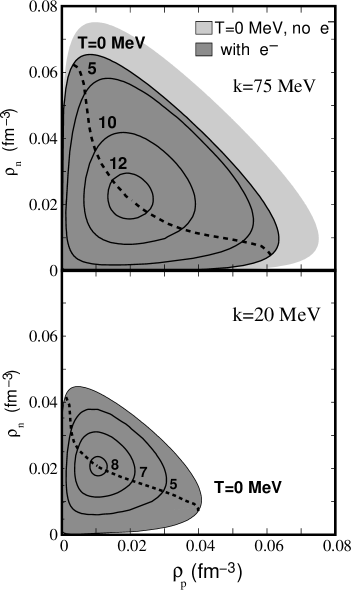
Figure 1: Spinodal sections for several temperatures and momentum transfer $k=75$ MeV and $k=20$ MeV.

In this section we present the results for the modes that define the instabilities of the system, corresponding to imaginary frequencies. We are interested in understanding the effect of the temperature and of the presence of electrons on these instabilities.

In Fig. 1 we plot the spinodal region for different temperatures and $k=20,\,75$ MeV. The second value of $k$ approximately defines the envelope of the spinodal region. We have also considered a smaller value of $k$ in order to get a larger effect of the electrons. As can be seen in Fig. 3, the influence of the electrons decreases, as $k$ increases up to $k\lesssim 70-80$ MeV/c (thick lines), similar to what happened at zero temperature. This is expected since the Coulomb contribution varies with the inverse of the momentum square, becoming weaker at large $k$. For higher values of $k$, this effect becomes negligible and we recover the behavior already observed in previous1 ; previous , i.e., the instability region decreases with the increase in the momentum transfer (thin lines). This is in fact coming from the finite range of the nuclear interaction which reduces the binding of the matter with a $k^{2}$ term and leads to a reduction of the spinodal region at large $k$. In a thermodynamical calculation of the spinodal for npe matter within the NL3 parametrization done in instabilities2 it was shown that above 2.4 MeV the instability region completely disappeared. In fact it is important to include electrons in a dynamical way and allow independent electron and proton density fluctuations in order to get the real behavior of the system. For $k=75$ MeV it is seen that an instability region exists for quite high temperatures, $T_{cr}=12.39$ MeV. The largest critical temperature is a function of $k$ and, as we discuss next, occurs for symmetric matter only for matter without electrons or for very large values of $k$, when the Coulomb field is negligible. The spinodals with $k=20$ MeV present several differences with respect to the $k=75$ MeV case: the critical temperature is lower, the range of densities corresponding to the instability region is smaller and, while for $k=75$ MeV the spinodals are practically symmetric with respect to equal proton/neutron concentrations, for $k=20$ MeV the spinodal sections have a larger contribution in the $\rho_{p}<\rho_{n}$ range.

Figure 2: The ratio $\frac{\delta\rho_{n}}{\delta\rho_{p}}$ at the critical points. Thin (thick) lines represent the critical points at the section $\rho_{p}>\rho_{n}$ ($\rho_{p}<\rho_{n}$).

Figure 3: Spinodal sections at T=0 and 10 MeV. The EoS for $\beta$-equilibrium matter is also shown.

In Fig. 1 we also include the line of critical points. These points of the spinodal are such that the associated eigenvector of the equations of motion is tangent to the spinodal curve. A very similar method was obtained to determine the critical points of the thermodynamical spinodal in instabilities2 . Again, it is clear the difference between the two values of $k$ discussed. In Fig. 2 we plot the ratio $\frac{\delta\rho_{n}}{\delta\rho_{p}}$ at which the critical point occurs. The lower branches (thin curves) for both cases correspond to the $\rho_{p}>\rho_{n}$ section while the upper branches (thick curves) to the $\rho_{p}<\rho_{n}$ section. For $k=75$ MeV the ratio of proton/neutron density fluctuations is practically parallel to the line of equal concentration of protons and neutrons ($\rho_{n}/\rho_{p}=1$), not much different from the behavior of np matter chomaz . However for $k=20$ MeV the eigenvectors at the instability border are tilted in the neutron direction, preventing a strong distillation effect.

Figure 4: The ratio of the neutron-density fluctuation over the proton-density fluctuation is plotted for $\rho=0.15\rho_{0}$ as a function of a) momentum for $T=0$ (thick) and 5 MeV (thin); b) temperature for $k=15$ (very thick line), 25 (thick line) and 75 MeV (thin line). In this figure the dotted line represents $\rho_{n}/\rho_{p}$ for $y_{p}=0.3$.

As already referred, in Fig. 3 we show the spinodal regions for different values of $k$ at $T=0$ and 10 MeV. We also include the equation of state (EoS) of stellar matter in $\beta$-equilibrium without neutrinos ($Y_{\nu_{e}}=0$) and with trapped neutrinos ($Y_{L}\not=0$). In this last case we have considered a constant leptonic fraction (electrons plus neutrinos) equal to $Y_{L}=0.4$, according to prak97 .

For T= 10 MeV, an unstable region only exists for $k~{}\hbox to0.0pt{$>$\hss}{\lower 4.30554pt\hbox{$\sim$}}\,30$ MeV and $k\lesssim 150$ MeV. The spinodal region is strongly asymmetric at small $k$ because of the electron stabilizing effect, it becomes almost symmetric at large $k$ with the reduction of the coupling with electrons. For T= 0 MeV it is also seen the strong asymmetry of the spinodal at k=5 MeV as compared to k=250 MeV when the effect of electrons is negligible.

The EoS of stellar matter in $\beta$ equilibrium crosses all the spinodal sections above $k$=6 MeV and below $k$=150 MeV at $T$=0 MeV indicating the existence of a nucleation phase at the crust of the star. The size of the inhomogeneities is of the order 8-200 fm. However, from Fig. 5 we see that the most unstable mode has $k=145$ MeV which corresponds to a modulation with $\lambda\sim 9$ fm. At $T$=10 MeV the $\beta$ equilibrium EoS does not cross the unstable region. At this temperature matter is homogeneous for all densities. However, for matter with trapped neutrinos the inhomogeneities are again present. In this case, the EoS crosses the unstable region even at $T$=10 MeV for 30 MeV$<k<137$ MeV and at $T$=0 MeV the spinodals are crossed for all values of $k$ for which the instabilities occur.

In Fig. 4a) the ratio of the neutron-density fluctuation over the proton-density fluctuation is plotted as a function of momentum for $T=0$ and 5 MeV and $y_{p}=0.5,\,0.3,\,0.2$ and $\rho=0.15\rho_{0}$. Comparing the finite temperature results with the zero temperature ones we conclude: a) for large $k$ the fluctuations are closer to the ratio $\rho_{n}/\rho_{p}$ and therefore, the distillation effect is not so efficient; b) the anti-distillation effects, $\frac{\delta\rho_{n}}{\delta\rho_{p}}>\frac{\rho_{n}}{\rho_{p}}$, settles in at larger values of $k$. This becomes more clear from Fig. 4b) and it is more pronounced for asymmetric matter. In particular for $y_{p}=0.3$ the ratio $\delta\rho_{n}/\delta\rho_{p}$ comes close to the value $\rho_{n}/\rho_{p}=2.33$ (denoted by the dotted line) for $k=25$ MeV and is completely above that value for $k=15$ MeV. It is also interesting to notice that for $k=15$ MeV, contrary to $k=25,\,75$ MeV, asymmetric matter ($y_{p}=0.3$) is more unstable at higher temperatures than symmetric matter. This point is discussed below together with Fig. 6.

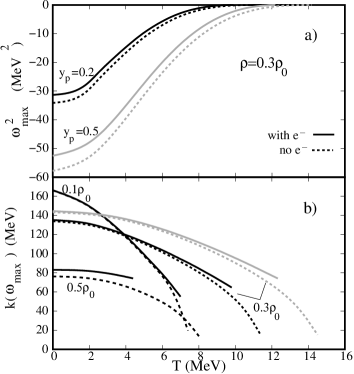
Figure 5: Most unstable mode as a function of temperature for: a) the square of the corresponding frequency at $\rho=0.3\rho_{0}$ and $y_{p}=0.2$ (black) and $y_{p}=0.5$ (grey); b) the momentum transfer at which the most unstable mode occurs for several densities and proton fractions (same colors as in a) ).

The most unstable mode (the one with the largest modulus of the imaginary frequency), indicating the existence of an instability, defines the behavior of the system, namely, the most probable size of the inhomogeneities which are formed due to the perturbation. In Fig. 5 we plot $\omega_{max}^{2}$ and the momentum $k$ at which this mode occurs as a functions of temperature and isospin asymmetry. The modulus of $\omega_{max}^{2}$ decreases with temperature, isospin asymmetry and the presence of electrons. This behavior is expected since any of these factors decreases the instability region of the system.

In Fig. 5b) we plot $k(\omega_{max})$ for the values of Fig. 5a) ($\rho=0.3\rho_{0}$ and $y_{p}=0.5,\,0.2$) and for $y_{p}=0.2$, $\rho=0.1\rho_{0}$ and $0.5\rho_{0}$. For the same density, the value of $k(\omega_{max})$ also decreases both with the increase of temperature and isospin asymmetry. This means that the effect of the electrons, which is more important for smaller $k$ values, is more effective at higher temperature values and larger asymmetries. For a given temperature, electrons shift the most unstable mode to slightly larger values of $k$. If we fix the proton fraction, $y_{p}=0.2$, and vary the density we conclude that close to the critical temperature the $k$ lies always in the interval 60-80 MeV. The large difference occurs at zero temperature: in this case the smaller the density the larger the value of $k$. These results seem to indicate that only under special conditions the electrons have a strong effect on the behavior of the system, since the most unstable mode has $k>60$ MeV and larger electron effects are expected for $k$ below this value as discussed next.

Figure 6: Critical a) temperatures, b) proton and neutron densities, as a function of momentum transfer including/not including electrons.

In Fig. 6 we plot the critical temperatures and densities as a function of the wave number of the perturbation for npe matter and nuclear (np) matter. For values of $k>150$ MeV the critical temperatures almost coincide. As expected, electrons decrease drastically the critical temperatures for small values of $k$. Another effect is a reduction of the critical density at low $k$ transfer which is more pronounced on the proton density than on the neutron density. A high proton density region will have a larger contribution from electrons which stabilize matter. We conclude that while at np matter the critical temperature occurs for symmetric matter, this is generally not anymore true if electrons are present. In fact, for large values of $k$ ($k>150$ MeV) matter is almost symmetric at $T=T_{cr}$, but for small values of $k$ we can have significant asymmetries for $yp\sim 0.25-0.4$ at the critical temperatures.

V Conclusions

In the present work, we have looked at the dynamical instabilities of nuclear neutral warm matter which is of interest for the study of neutron stars and supernovae. In particular, we have studied the effect of the temperature and the inclusion of the Coulomb interaction on the instability region of nuclear matter. The calculations were performed within a relativistic mean-field approach to nuclear matter, namely the NL3 parametrization of the NLWM but we believe that the main conclusions with respect to the dynamical instabilities would be similar if obtained within other models with constant couplings taking into account the results of previous1 .

We may interpret the present calculation as a way of going beyond a total screening effect calculation which considers equal distributions of electron and proton clouds. On the other hand, no electron screening would correspond to an homogeneous distribution of electrons. We have seen that for small $k$ transfers, electrons and protons stick together which corresponds to a large screening effect. On the other hand for large momentum transfers protons and electrons behave independently and this corresponds to the no screening limit.

For np matter it was shown that the largest critical temperatures above which nuclear matter is stable occurs for symmetric matter. This is not anymore true for npe matter: critical temperatures occur for asymmetric matter with $yp<0.5$. The critical proton fraction can be as low as 0.22 for $k=8$ MeV, where $T_{cr}\simeq 4.5$ MeV.

In wata04 the structure of hot dense matter at subnuclear densities has been investigated by quantum molecular dynamics (QMD) simulations. In this work the critical temperature for the phase separation is $~{}\hbox to0.0pt{$>$\hss}{\lower 4.30554pt\hbox{$\sim$}}6$ MeV for the proton fraction $y_{p}=0.5$ and $~{}\hbox to0.0pt{$>$\hss}{\lower 4.30554pt\hbox{$\sim$}}5$ MeV for $y_{p}=0.3$. These results seem to be compatible with Fig 6. In our approach we get for $y_{p}=0.3$ a critical temperature of 5 MeV at $k=10$ MeV. The maximum critical temperature is 12.38 MeV and occurs for $y_{p}=0.47$ at $k=75$ MeV. For npe matter with $y_{p}>0.495$ the critical temperature occurs at $T\lesssim 8.5$ MeV for $k>180$ MeV.

We have seen that stellar matter with trapped neutrinos is more affected by the presence of a non-homogeneous phase than neutrino free stellar matter. We have also concluded that at finite temperature the distillation effect in asymmetric matter is not so efficient, and in particular the anti-distillation effect defined as $\frac{\delta\rho_{n}}{\delta\rho_{p}}>\frac{\rho_{n}}{\rho_{p}}$, which occurs at small $k$, settles in at larger values of $k$. We may expect this effect to have consequences in warm stellar matter. In a supernovae explosion 99% of the energy of the collapse is radiated away in neutrinos. Neutrinos interact strongly with neutrons because of the large weak vector charge of the neutron. Therefore, the way neutrons clusterize is important to determine the neutrino mean free path. These neutrinos may couple strongly to the neutron-rich matter low-energy modes present in this explosive environment ksg , and in this way revive the stalled supernovae shock.

The wavelength of the modulations which correspond to the most unstable modes increases with temperature. While for $T=0$ MeV the presence of electrons has almost no effect due to the high values of $k$ ($\sim 125-145$ MeV), for asymmetric matter close to the critical temperatures they really make some difference. These are temperatures and proton fractions of the order of the ones found in stellar matter of protoneutron stars and therefore will affect the crust formation and the neutrino diffusion during the cooling process.

The results we have obtained are intimately related with the studies developed in hpbp ; horo2 ; maru , where the nuclear pasta is generally modeled as a charge neutral system of protons, neutrons and electrons at subnuclear densities. In horo2 one sees that, for small momentum transfers, the dynamical response function shows a peak, identified as a plasmon mode, and displays an important amount of strength at low energies identified as a coherent density wave. In this work a fixed screening length of 10 fm was considered. Small momentum transfers are precisely the ones for which protons are more influenced by the presence of electrons and therefore a carefull calculation taking into account this point should be carried out.

In maru the authors have compared different treatments of Coulomb interaction: in particular they have shown that the full and the no electron screening calculations give similar results demonstrating the weakness of the electron-screening effects. We came also to a similar conclusion, however we could identify under which conditions the electron-screening effects are important, namely for small $k$ transfers.

In previous1 it was shown that density dependent hadronic models have different behaviors from the NLWM we have studied in the present work, coming closer to non-relativisitc nuclear models with Skyrme forces. The dynamical instabilities of npe matter within these models is currently under investigation. The calculation of collective modes of neutron-rich nuclear clusters immersed in a gas of neutrons, including electrons dynamically, should also be studied.

Appendix A Equations for the fields

$$\frac{\partial^{2}\phi}{\partial t^{2}}-\nabla^{2}\phi+m_{s}^{2}\phi+\frac{\kappa}{2}\phi^{2}+\frac{\lambda}{6}\phi^{3}=g_{s}\rho_{s}({\bf r},t)\;,$$ (23)

$$\frac{\partial^{2}V_{0}}{\partial t^{2}}-\nabla^{2}V_{0}+m_{v}^{2}V_{0}\,=\,g_{v}j_{0}({\bf r},t)\;,$$ (24)

$$\frac{\partial^{2}V_{i}}{\partial t^{2}}-\nabla^{2}V_{i}+m_{v}^{2}V_{i}\,=\,g_{v}j_{i}({\bf r},t)\;,$$ (25)

$$\frac{\partial^{2}b_{0}}{\partial t^{2}}-\nabla^{2}b_{0}+m_{\rho}^{2}b_{0}\,=\,\frac{g_{\rho}}{2}j_{3,0}({\bf r},t)\;,$$ (26)

$$\frac{\partial^{2}b_{i}}{\partial t^{2}}-\nabla^{2}b_{i}+m_{v}^{2}b_{i}\,=\,\frac{g_{\rho}}{2}j_{3,i}({\bf r},t)\;,$$ (27)

$$\frac{\partial^{2}A_{0}}{\partial t^{2}}-\nabla^{2}A_{0}\,=\,e[j_{0p}({\bf r},t)-j_{0e}({\bf r},t)]\;,$$ (28)

$$\frac{\partial^{2}A_{i}}{\partial t^{2}}-\nabla^{2}A_{i}\,=\,e[j_{pi}({\bf r},t)-j_{ei}({\bf r},t)]\;,$$ (29)

where the scalar density is

$$\rho_{s}({\bf r},t)=2\sum_{i=p,n}\int\frac{d^{3}p}{(2\pi)^{3}}\,(f_{i+}({\bf r},{\bf p},t)+f_{i-}({\bf r},{\bf p},t))\,\frac{M^{*}}{\epsilon_{i}}\;.$$ (30)

The components of the baryonic four-current density are

$$j_{0}({\bf r},t)=2\sum_{i=p,n}\int\frac{d^{3}p}{(2\pi)^{3}}\,(f_{i+}({\bf r},{\bf p},t)-f_{i-}({\bf r},{\bf p},t))\;,$$ (31)

$${\bf j}({\bf r},t)=2\sum_{i=p,n}\int\frac{d^{3}p}{(2\pi)^{3}}\,(f_{i}({\bf r},{\bf p},t)+f_{i-}({\bf r},{\bf p},t))\frac{{\bf p}-\boldsymbol{\cal V}_{i}}{\epsilon_{i}}\;,$$ (32)

$$j_{0e}({\bf r},t)=2\int\frac{d^{3}p}{(2\pi)^{3}}\,(f_{e+}({\bf r},{\bf p},t)-f_{e-}({\bf r},{\bf p},t))\;,$$ (33)

$${\bf j}_{e}({\bf r},t)=2\int\frac{d^{3}p}{(2\pi)^{3}}\,(f_{e+}({\bf r},{\bf p},t)+f_{e-}({\bf r},{\bf p},t))\,\frac{{\bf p}+e\boldsymbol{\mathbf{A}}}{\epsilon_{e}}\;,$$ (34)

and the components of the isovector four-current density are

$$j_{3,0}({\bf r},t)=2\sum_{i=p,n}\int\frac{d^{3}p}{(2\pi)^{3}}\,\tau_{i}(f_{i+}({\bf r},{\bf p},t)-f_{i-}({\bf r},{\bf p},t))\;,$$ (35)

$${\bf j}_{3}({\bf r},t)=2\sum_{i=p,n}\int\frac{d^{3}p}{(2\pi)^{3}}\,\frac{{\bf p}-\boldsymbol{\cal V}_{i}}{\epsilon_{i}}\,\tau_{i}\;(f_{i+}({\bf r},{\bf p},t)+f_{i-}({\bf r},{\bf p},t))\;,$$ (36)

with $\epsilon_{i}=\sqrt{({\bf p}-\boldsymbol{\cal V}_{i})^{2}+{M^{*}}^{2}}\;,i=p,n$ and $\epsilon_{e}=\sqrt{({\bf p}+e{\mathbf{A}})^{2}+m_{e}^{2}}\;.$

Appendix B Linearized equations for the fields

$$\frac{\partial^{2}\delta\phi}{\partial t^{2}}-\nabla^{2}\delta\phi+(m_{s}^{2}+\kappa\phi_{0}+\frac{\lambda}{2}\phi_{0}^{2})\delta\phi\,=\,g_{s}\,\delta\rho_{s}\;,$$ (37)

$$\frac{\partial^{2}\delta V_{0}}{\partial t^{2}}-\nabla^{2}\delta V_{0}+m_{v}^{2}\delta V_{0}\,=\,g_{v}\,\delta j_{0}\;,$$ (38)

$$\frac{\partial^{2}\delta V_{i}}{\partial t^{2}}-\nabla^{2}\delta V_{i}+m_{v}^{2}\delta V_{i}\,=\,g_{v}\,\delta j_{i}\;,$$ (39)

$$\frac{\partial^{2}\delta b_{0}}{\partial t^{2}}-\nabla^{2}\delta b_{0}+m_{\rho}^{2}\delta b_{0}\,=\,\frac{g_{\rho}}{2}\,\delta j_{3,0}\;,$$ (40)

$$\frac{\partial^{2}\delta b_{i}}{\partial t^{2}}-\nabla^{2}\delta b_{i}+m_{\rho}^{2}\delta b_{i}\,=\,\frac{g_{\rho}}{2}\,\delta j_{3,i}\;,$$ (41)

$$\frac{\partial^{2}\delta A_{0}}{\partial t^{2}}-\nabla^{2}\delta A_{0}\,=\,e\,\left[\delta j_{0p}-\delta j_{0e}\right]\;,$$ (42)

$$\frac{\partial^{2}\delta A_{i}}{\partial t^{2}}-\nabla^{2}\delta A_{i}\,=\,e\,\left[\delta j_{pi}-\delta j_{ei}\right]\;,$$ (43)

with

$$\delta\rho_{s}=2\sum_{i=p,n}\int\frac{d^{3}p}{(2\pi)^{3}}\,\frac{M^{*}}{\epsilon}(\delta f_{i+}+\delta f_{i-})-\,g_{s}\delta\phi~{}{d\,\rho_{s}^{0}}\;,$$

$$\delta j_{0}=2\sum_{i=p,n}\int\frac{d^{3}p}{(2\pi)^{3}}\,(\delta f_{i+}-\delta f_{i-})$$

$$\delta{\mathbf{j}} = 2\sum_{i=p,n}\int\frac{d^{3}p}{(2\pi)^{3}}\ \frac{\mathbf{p}}{\epsilon}(\delta f_{i+}+\delta f_{i-})\,$$

$$- \,2\sum_{i=p,n}\int\frac{d^{3}p}{(2\pi)^{3}}\,(f_{0i+}+f_{0i-})\left(\frac{\delta\boldsymbol{\cal V}_{i}}{\epsilon}-\mathbf{p}\frac{{\mathbf{p}}\cdot\delta{\boldsymbol{\cal V}_{i}}}{\epsilon^{3}}\right)\;,$$

$$\delta j_{3,0}=2\sum_{i=p,n}\int\frac{d^{3}p}{(2\pi)^{3}}\,\tau_{i}\,(\delta f_{i+}-\delta f_{i-}),$$

$$\delta{\mathbf{j}}_{3} = 2\sum_{i=p,n}\int\frac{d^{3}p}{(2\pi)^{3}}\,\tau_{i}\,\frac{\mathbf{p}}{\epsilon}(\delta f_{i+}+\delta f_{i-})\,$$

$$- \,2\sum_{i=p,n}\int\frac{d^{3}p}{(2\pi)^{3}}\,\tau_{i}\,(f_{0i+}+f_{0i-})\left(\frac{\delta\boldsymbol{\cal V}}{\epsilon}-\mathbf{p}\frac{{\mathbf{p}}\cdot\delta{\boldsymbol{\cal V}}}{\epsilon^{3}_{0}}\right)\;.$$

$$\delta j_{0e}=2\int\frac{d^{3}p}{(2\pi)^{3}}\,(\delta f_{e+}-\delta f_{e-})\;,$$

$$\delta{\mathbf{j}}_{e} = 2\int\frac{d^{3}p}{(2\pi)^{3}}\,\,(\delta f_{e+}+\delta f_{e-})\,\frac{\mathbf{p}}{\epsilon_{0e}}\,$$

$$+ 2e\int\frac{d^{3}p}{(2\pi)^{3}}\,\,(f_{0e+}+f_{0e-})\left(\frac{\delta{\mathbf{A}}}{\epsilon_{0e}}-\mathbf{p}\frac{{\mathbf{p}}\cdot\delta{{\mathbf{A}}}}{\epsilon^{3}_{0e}}\right)\;.$$

Appendix C Dispersion relation

The dispersion relation is obtained from the determinant of the following set of five equations

$$\left(\begin{array}[]{ccccc}a_{11}&a_{12}&a_{13}&a_{14}&a_{15}\\ a_{21}&a_{22}&a_{23}&a_{24}&0\\ a_{31}&a_{32}&a_{33}&a_{34}&a_{35}\\ a_{41}&a_{42}&a_{43}&a_{44}&0\\ 0&0&a_{53}&0&a_{55}\\ \end{array}\right)\left(\begin{array}[]{c}\rho^{S}_{\omega p}\\ \rho^{S}_{\omega n}\\ \rho_{\omega p}\\ \rho_{\omega n}\\ \rho_{\omega e}\end{array}\right)=0.$$

The coeficients $a_{ij}$ are given by

$$a_{11}=1+c_{s}\left(I_{\omega+}^{0p}-I_{\omega-}^{0p}\right),$$

$$a_{21}=c_{s}\left(I_{\omega+}^{0p}-I_{\omega-}^{0p}\right),\,$$

$$a_{31}=-(c_{v}+c_{\rho}+c_{e})\left(I_{\omega+}^{1p}+I_{\omega-}^{1p}\right),\,$$

$$a_{41}=-(c_{v}-c_{\rho})\left(I_{\omega+}^{1p}+I_{\omega-}^{1p}\right),$$

$$a_{51}=c_{e}\left(I_{\omega+}^{1p}+I_{\omega-}^{1p}\right)$$

$$a_{21}=c_{s}\left(I_{\omega+}^{0n}-I_{\omega-}^{0n}\right),\,$$

$$a_{22}=1+c_{s}\left(I_{\omega+}^{0n}-I_{\omega-}^{0n}\right),\,$$

$$a_{23}=-(c_{v}-c_{\rho})\left(I_{\omega+}^{1n}+I_{\omega-}^{1n}\right),\,$$

$$a_{24}=-(c_{v}+c_{\rho})\left(I_{\omega+}^{1n}+I_{\omega-}^{1n}\right),\,$$

$$a_{25}=0$$

$$a_{31}=+c_{s}\left(I_{\omega+}^{1p}+I_{\omega-}^{1p}\right),\,$$

$$a_{32}=+c_{s}\left(I_{\omega+}^{1p}+I_{\omega-}^{1p}\right),\,$$

$$a_{33}=1-(c_{v}+c_{\rho}+c_{e})\left(I_{\omega+}^{2p}-I_{\omega-}^{2p}\right),\,$$

$$a_{34}=-(c_{v}-c_{\rho})\left(I_{\omega+}^{2p}-I_{\omega-}^{2p}\right)$$

$$a_{35}=c_{e}\left(I_{\omega+}^{2p}-I_{\omega-}^{2p}\right)$$

$$a_{41}=c_{s}\left(I_{\omega+}^{1n}+I_{\omega-}^{1n}\right),\,$$

$$a_{42}=c_{s}\left(I_{\omega+}^{1n}+I_{\omega-}^{1n}\right),\,$$

$$a_{43}=-(c_{v}-c_{\rho})\left(I_{\omega+}^{2n}-I_{\omega-}^{2n}\right),\,$$

$$a_{44}=1-(c_{v}+c_{\rho})\left(I_{\omega+}^{2n}-I_{\omega-}^{2n}\right),$$

$$a_{51}=a_{52}=a_{54}=0,\,$$

$$a_{53}=c_{e}\left(I_{\omega+}^{2e}-I_{\omega-}^{2e}\right),\,$$

$$a_{55}=1-c_{e}\left(I_{\omega+}^{2e}-I_{\omega-}^{2e}\right)$$

where we have defined the following quantities

$$c_{s}=\frac{2G_{1}^{2}}{(2\pi)^{2}T}\frac{1}{\bar{\omega}^{2}-\omega_{s}^{2}},\qquad\bar{\omega}_{s}^{2}=(k^{2}+m^{2}_{s,eff})/k^{2},$$

$$c_{v}=\frac{2}{(2\pi)^{2}T}\frac{1}{\bar{\omega}^{2}-\bar{\omega}_{v}^{2}}\left(\frac{g_{v}}{k}\right)^{2}(1-\bar{\omega}^{2}),\qquad\omega_{v}^{2}=(k^{2}+m_{v}^{2})/k^{2},$$

$$c_{\rho}=\frac{2}{(2\pi)^{2}T}\frac{1}{\bar{\omega}^{2}-\bar{\omega}_{\rho}^{2}}\left(\frac{g_{\rho}}{2k}\right)^{2}(1-\bar{\omega}^{2}),\qquad\omega_{\rho}^{2}=(k^{2}+m_{\rho}^{2})/k^{2},$$

$$c_{e}=\frac{-2}{(2\pi)^{2}T}\left(\frac{e}{k}\right)^{2}$$

$$\bar{\omega}=\frac{\omega}{k},\quad x=\frac{p\cos\theta}{\epsilon},\quad G_{1}=\frac{g_{s}M^{*}}{k}.$$

$$I_{\omega_{\mp}}(\epsilon)=\int_{-p/\epsilon}^{p/\epsilon}~{}dx\frac{x}{\bar{\omega}\pm x}=\pm\left[2\frac{p}{\epsilon}+\bar{\omega}~{}ln\left|\frac{\bar{\omega}-p/\epsilon}{\bar{\omega}+p/\epsilon}\right|\right]$$

$$I^{ni}_{\omega_{\mp}}=\int_{M^{*}}^{\infty}\epsilon^{n}I_{\omega_{\mp}}(\epsilon)f_{0i\mp}(f_{0i\mp}-1)d\epsilon.$$

The amplitudes $\rho^{S}_{\omega i}$ and $\rho_{\omega i}$ are given by

$$\rho_{\omega i}^{S}=A^{1}_{\omega i,+}-A^{1}_{\omega i,-},$$ (44)

$$\rho_{\omega i}=A^{0}_{\omega i,+}+A^{0}_{\omega i,-}$$ (45)

where

$$A_{\omega i,\pm}^{n}=\int_{M^{*}}^{\infty}\epsilon^{n}d\epsilon\int_{-p/\epsilon}^{p/\epsilon}dx\,x\,S_{\omega\pm}^{i}(x,p)\,f_{0i\pm}\left(f_{0i\pm}-1\right).$$ (46)

At low densities, corresponding to a negative value of the compressibility, the system presents unstable modes characterized by an imaginary frequency. In order to obtain these modes, one has to replace $\bar{\omega}$ by $i\beta$. In this case, the integrals $I_{\omega_{\mp}}(\epsilon)$ become

$$I_{\beta_{\mp}}(\epsilon)=\pm\left[2\frac{p}{\epsilon}-2\beta\tan^{-1}(p/\epsilon\beta).\right]$$ (47)

References

• (1) S.S. Avancini, L. Brito, D.P. Menezes and C. Providência, Phys. Rev. C 70, 015203 (2004).
• (2) S.S. Avancini, L. Brito, D.P. Menezes and C. Providência, Phys. Rev. C 71, 044323 (2005).
• (3) C. Providência, D.P. Menezes and L. Brito, Nucl. Phys. A 703, 188 (2002); D.P. Menezes and C. Providência, Phys. Rev. C 64, 044306 (2001); D.P. Menezes and C. Providência, Nucl. Phys. A 650, 283 (1999); D.P. Menezes and C. Providência, Phys. Rev. C 60, 024313 (1999).
• (4) D. G. Ravenhall, C. J. Pethick, and J. R. Wilson, Phys. Rev. Lett. 50, 2066 (1983); M. Hashimoto, H. Seki, and M. Yamada, Prog. Theor. Phys.71, 320 (1984).
• (5) C. J. Horowitz, M. A. Perez-Garcia, and J. Piekarewicz, Phys. Rev. C 69, 045804 (2004).
• (6) G. Watanabe, K. Sato, K. Yasuoka, and T. Ebisuzaki, Phys. Rev. C 69, 055805 (2004); G. Watanabe, T. Maruyama, K. Sato, K. Yasuoka, and T. Ebisuzaki, Phys. Rev. Lett. 94, 031101 (2005).
• (7) T. Maruyama, T. Tatsumi, D. N. Voskresensky, T. Tanigawa, and S. Chiba, Phys. Rev. C 72, 015802 (2005).
• (8) C. J. Horowitz, M. A. Perez-Garcia, D. K. Berry, and J. Piekarewicz, Phys. Rev. C 72, 035801 (2005); C. J. Horowitz, M. A. Perez-Garcia, J. Carriere, D. K. Berry, and J. Piekarewicz, Phys. Rev. C 70, 065806 (2004).
• (9) R. F. Sawyer, Phys. Rev. D 11, 2740 (1975); N. Iwamoto and C. J. Pethick, Phys. Rev. D 25, 313 (1982).
• (10) S. Reddy, G. Bertsch and M. P. Prakash, Phys. Lett. B 475, 1 (2000).
• (11) C. Providência, L. Brito, S.S. Avancini, D. P. Menezes, Ph. Chomaz, Phys. Rev. C 73, 025805 (2006).
• (12) E. Khan, N. Sandulescu, and Nguyen Van Giai, Phys. Rev. C 71, 042801(R) (2005).
• (13) M. Nielsen, C. Providência and J. da Providência, Phys. Rev. C 44, 209 (1991)
• (14) M. Nielsen, C. da Providência, J. da Providência and Wang-Ru Lin, Mod. Phys. Lett. A 10, 919 (1994); M. Nielsen, C. Providência and J. da Providência, Phys. Rev. C 47, 200 (1993).
• (15) G. A. Lalazissis, J. König and P. Ring, Phys. Rev. C 55, 540 (1997).
• (16) S.S. Avancini, L. Brito, Ph. Chomaz, D.P. Menezes, and C. Providência, submitted to publication.
• (17) J. Margueron and P. Chomaz, Phys. Rev. C 67, 041602(R) (2003); P. Chomaz, M. Colonna and J. Randrup, Phys. Rep. 389, 263 (2004).
• (18) M. Prakash, I. Bombaci, M. Prakash, P. J. Ellis, J. M. Lattimer and R. Knorren, Phys. Rep. 280, 1 (1997).