Baryon Number and Electric Charge Fluctuations
in Pb+Pb Collisions at SPS energies

Abstract

Event-by-event fluctuations of the net baryon number and electric charge in nucleus-nucleus collisions are studied in Pb+Pb at SPS energies within the HSD transport model. We reveal an important role of the fluctuations in the number of target nucleon participants. They strongly influence all measured fluctuations even in the samples of events with rather rigid centrality trigger. This fact can be used to check different scenarios of nucleus-nucleus collisions by measuring the multiplicity fluctuations as a function of collision centrality in fixed kinematical regions of the projectile and target hemispheres. The HSD results for the event-by-event fluctuations of electric charge in central Pb+Pb collisions at 20, 30, 40, 80 and 158 A GeV are in a good agreement with the NA49 experimental data and considerably larger than expected in a quark-gluon plasma. This demonstrate that the distortions of the initial fluctuations by the hadronization phase and, in particular, by the final resonance decays dominate the observable fluctuations.

I Introduction

The aim of the present paper is to study the fluctuations of the net baryon number and electric charge in nucleus-nucleus (A+A) collisions at SPS energies. We use the HSD HSD transport approach which reproduces both the different particle multiplicities and longitudinal differential rapidity distributions for central collisions of Au+Au (or Pb+Pb) from AGS to SPS energies rather well Weber . (see, e.g., Refs. fluc1 ; fluc2 ; fluc3 ; fluc4 ; fluc5 ; fluc6 ; fluc7 ; fluc7a ; fluc7b ; fluc8 and references therein) reveal a new physical information. The fluctuations in A+A collisions are studied on an event-by-event basis: a given observable is measured in each event and the fluctuations are evaluated for a specially selected set of these events. We recall that the statistical model has been successfully used to describe the data on hadron multiplicities in relativistic A+A collisions (see, e.g., Ref. stat1 and a recent review BMST ) as well as in elementary particle collisions stat2 . This gives rise to the question whether the fluctuations, in particular the multiplicity fluctuations, do also follow the statistical hadron-resonance gas results. Recently the particle number fluctuations have been studied in different statistical ensembles stat3 ; the statistical fluctuations can be closely related to phase transitions in QCD matter, with specific signatures for 1-st and 2-nd order phase transitions as well as for the critical point fluc4 ; fluc5 .

In addition to the statistical fluctuations the complicated time evolution of A+A collisions generates dynamical fluctuations. The fluctuations in the initial energy deposited inelastically in the statistical system yield dynamical fluctuations of all macroscopic parameters, like the total entropy or strangeness content. The observable consequences of the initial energy density fluctuations are sensitive to the equation of state, and can therefore be useful as signals for phase transitions fluc8 . Even when the data are obtained with a centrality trigger the number of nucleons participating in inelastic collisions still fluctuates considerably. In the language of statistical mechanics, these fluctuations in the participant nucleon number correspond to volume fluctuations. Secondary particle multiplicities scale linearly with the volume, hence, volume fluctuations translate directly to particle number fluctuations.

The present work is a continuation of our recent study KGB where we have analyzed the charged particle number fluctuations in Pb+Pb collisions at 158 AGeV within the UrQMD and HSD transport approaches. The net baryon number and electric charge event-by-event fluctuations are studied in different rapidity regions of the projectile and target hemispheres.

The paper is organized as follows. Section II presents the HSD results for the fluctuations of the number of nucleon participants while Sections III and IV give the net baryon number fluctuations and electric charge fluctuations, respectively. In Section V we discuss the fluctuations in the samples of most central collisions, Section VI shows a comparison of our calculations with experimental data from the NA49 Collaboration, whereas Section VII finally concludes the present study.

II Fluctuations of the Number of Participants

In each A+A collision only a fraction of all 2$A$ nucleons interact. These are called participant nucleons and are denoted as $N_{P}^{proj}$ and $N_{P}^{targ}$ for the projectile and target nuclei, respectively. The nucleons, which do not interact, are called the projectile and target spectators, $N_{S}^{proj}=A-N_{P}^{proj}$ and $N_{S}^{targ}=A-N_{P}^{targ}$. The fluctuations in high energy A+A collisions are dominated by a geometrical variation of the impact parameter. However, even for the fixed impact parameter the number of participants, $N_{P}\equiv N_{P}^{proj}+N_{P}^{targ}$, fluctuates from event to event. This is due to the fluctuations of the initial states of the colliding nuclei and the probabilistic character of the interaction process. The fluctuations of $N_{P}$ form usually a large and uninteresting background. In order to minimize its contribution the NA49 Collaboration has selected samples of collisions with a fixed numbers of projectile participants. This selection is possible due to a measurement of $N_{S}^{proj}$ in each individual collision by a calorimeter which covers the projectile fragmentation domain. However, even in the samples with $N_{P}^{proj}=const$ the number of target participants fluctuates considerably. Hence, an asymmetry between projectile and target participants is introduced, i.e. $N_{P}^{proj}$ is constant by constraint, whereas $N_{P}^{targ}$ fluctuates independently.

In the following the variance, $Var(n)\equiv\langle n^{2}\rangle-\langle n\rangle^{2}$, and scaled variance, $\omega_{n}\equiv Var(n)/\langle n\rangle$, where $n$ stands for a given random variable and $\langle\cdots\rangle$ for event-by-event averaging, will be used to quantify fluctuations. In each sample with $N_{P}^{proj}=const$ the number of target participants fluctuates around its mean value, $\langle N_{P}^{targ}\rangle$ with the scaled variance $\omega_{P}^{targ}$. From an output of the HSD minimum bias simulations of Pb+Pb collisions at 158 AGeV we form the samples of events with fixed values of $N_{P}^{proj}$. Fig. 1 presents the HSD average value $\langle N_{P}^{targ}\rangle$ (left) and the scaled variances $\omega_{P}^{targ}$ (right) as functions of $N_{P}^{proj}$. One finds $\langle N_{P}^{targ}\rangle\simeq N_{P}^{proj}$; the deviations are only seen at very small ($N_{P}^{proj}\approx 1$) and very large ($N_{P}^{proj}\approx A$) numbers of projectile participants. The fluctuations of $N_{P}^{targ}$ are quite strong: $\omega_{P}^{targ}>2$ at $N_{P}^{proj}=10-80$.

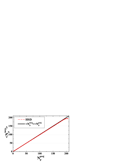
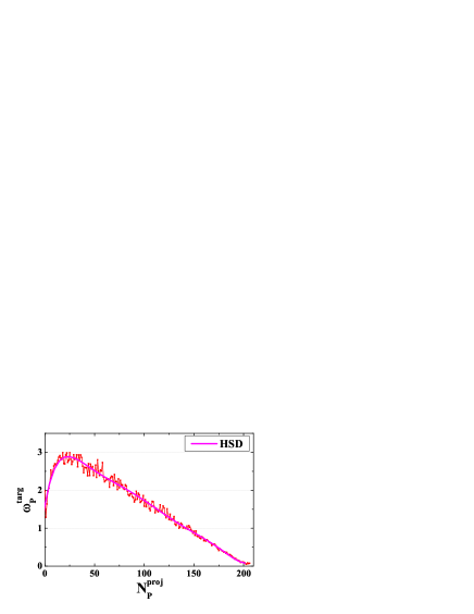
Figure 1: The HSD simulations in Pb+Pb collisions at 158 AGeV for the average value $\langle N_{P}^{targ}\rangle$ (left) and the scaled variances $\omega_{P}^{targ}$ (right) as functions of $N_{P}^{proj}$.

The consequences of the asymmetry between projectile and target hemispheres depend on the A+A dynamics. According to Ref. MGMG different models of hadron production in relativistic A+A collisions can be divided into three limiting groups: transparency (T-), mixing (M-), and reflection (R-) models. The rapidity distributions resulting from the T-, M-, and R-models are sketched in Fig. 2 taken from Ref. MGMG . We note that there are models which assume the mixing of hadron production sources, however, the transparency of baryon flows, e.g. three-fluid hydrodynamical model 3fluid . R-models appear rather unrealistic and are included for completeness in our discussion.

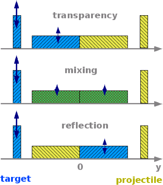
Figure 2: The sketch of the rapidity distributions of the baryon number or the particle production sources (horizontal rectangles) in nucleus-nucleus collisions resulting from the transparency, mixing and reflection models. The spectator nucleons are indicated by the vertical rectangles. In the collisions with a fixed number of projectile spectators only matter related to the target shows significant fluctuations (vertical arrows). See Ref. MGMG for more details.

III Net Baryon Number Fluctuations

We begin with a quantitative discussion by first considering the fluctuations of the net baryon number in different regions of the participant domain in collisions of two identical nuclei. These fluctuations are most closely related to the fluctuations of the number of participant nucleons because of baryon number conservation.

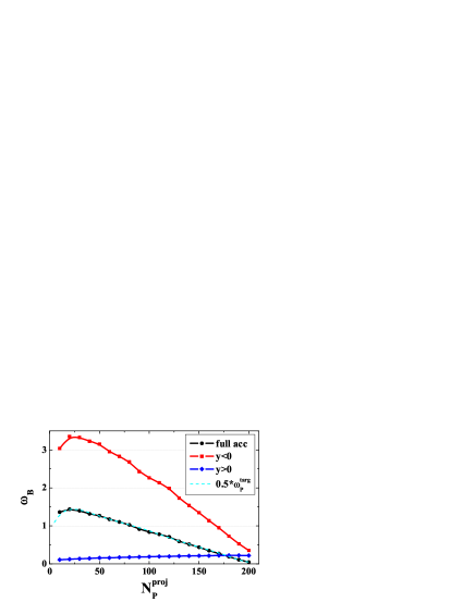
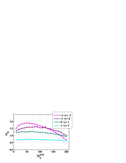
Figure 3: The HSD simulations for Pb+Pb collisions at 158 AGeV for fixed values of $N_{P}^{proj}$. Left: The baryon number fluctuations in full acceptance, $\omega_{B}$, in projectile hemisphere, $\omega_{B}^{p}$ (lower curve), and in target hemisphere, $\omega_{B}^{t}$ (upper curve). The dashed line, $0.5~{}\omega_{P}^{targ}$, demonstrates the validity of the relation (1). Right: The scaled variances of the baryon number fluctuations in different rapidity intervals.

The HSD results for $\omega_{B}$ in Pb+Pb at 158 AGeV are presented in Fig. 3. In each event we subtract the nucleon spectators when counting the number of baryons. The net baryon number in the full phase space, $B\equiv N_{B}-N_{\overline{B}}$, equals then to the total number of participants $N_{P}=N_{P}^{targ}+N_{P}^{proj}$. At fixed $N_{P}^{proj}$ the $N_{P}$ number fluctuates due to fluctuations of $N_{P}^{targ}$. These fluctuations correspond to an average value, $\langle N_{P}^{targ}\rangle\simeq N_{P}^{proj}$, and a scaled variance, $\omega_{P}^{targ}$ (see Fig. 1). Thus, for the net baryon number fluctuations in the full phase space we find,

$$\omega_{B}~{}=~{}\frac{Var(N_{P})}{\langle N_{P}\rangle}~{}\simeq~{}\frac{\langle\left(N_{P}^{targ}\right)^{2}\rangle~{}-~{}\langle N_{P}^{targ}\rangle^{2}}{2\langle N_{P}^{targ}\rangle}~{}=~{}\frac{1}{2}~{}\omega_{P}^{targ}~{}.$$ (1)

A factor $1/2$ in the right hand side of Eq. (1) appears because only half of the total number of participants fluctuates.

Let us introduce $\omega_{B}^{p}$ and $\omega_{B}^{t}$, where the superscripts $p$ and $t$ mark quantities measured in the projectile and target momentum hemispheres, respectively. Fig. 3 demonstrates that $\omega_{B}^{t}>\omega_{B}^{p}$, both in the whole projectile-target hemispheres and in the symmetric rapidity intervals. On the other hand one observes that $\omega_{B}^{p}\approx\omega_{B}^{t}$ in most central collisions. This is because the fluctuations of the target participants become negligible in this case, i.e. $\omega_{P}^{targ}\rightarrow 0$ (Fig. 1, right). As a consequence the fluctuations of any observable in the symmetric rapidity intervals become identical in most central collisions. Note also that transparency-mixing effects are different at different rapidities. From Fig. 1 (right) it follows that $\omega_{B}^{p}$ in the target rapidity interval $[-2,-1]$ is much larger than $\omega_{B}^{t}$ in the symmetric projectile rapidity interval $[1,2]$. This fact reveals the strong transparency effects. On the other hand, the behavior is different in symmetric rapidity intervals near the midrapidity. From Fig. 1 (right) one observes that $\omega_{B}^{p}$ in the target rapidity interval $[-1,0]$ is already much closer to $\omega_{B}^{t}$ in the symmetric projectile rapidity interval $[0,1]$. This gives a rough estimate of the width, $\Delta y\approx 1$, for the region in rapidity space where projectile and target nucleons communicate to each others.

By assumption, the mixing of the projectile and target participants is absent in T- and R-models. Therefore, in T-models, the net baryon number in the projectile hemisphere equals to $N_{p}^{proj}$ and does not fluctuate, i.e. $\omega_{B}^{p}(T)=0$, whereas the net baryon number in the target hemisphere equals to $N_{p}^{targ}$ and fluctuates with $\omega_{B}^{t}(T)=\omega_{P}^{targ}$. These relations are reversed in R-models. We introduce now a mixing of baryons between the projectile and target hemispheres. Let $\alpha$ be the probability for a (projectile) target participant to be detected in the (target) projectile hemisphere. We denote by $n^{t}$ and $n^{p}$ the number of baryons which end uo in the target and projectile hemisphere, respectively, from the opposite hemisphere. Then the probabilities to detect $B^{t}$ baryons in the target hemisphere, and $B^{p}$ baryons in the projectile hemisphere, can be written as,

$$P(B^{t};N_{P}^{proj})~{}=~{}\sum_{N_{P}^{targ}}W(N_{P}^{targ};N_{P}^{proj})~{}\sum_{n^{t}=1}^{N_{P}^{targ}}\sum_{n^{p}=1}^{N_{P}^{proj}}\alpha^{n^{p}}(1-\alpha)^{N_{P}^{targ}-n^{p}}~{}\frac{N_{P}^{targ}!}{n^{p}!(N_{P}^{targ}-n^{p})!}$$

$$\times~{}\alpha^{n^{t}}(1-\alpha)^{N_{P}^{proj}-n^{t}}~{}\frac{N_{P}^{proj}!}{n^{t}!(N_{P}^{proj}-n^{t})!}~{}\delta\left(B^{t}-N_{P}^{targ}~{}-n^{t}~{}+~{}n^{p}\right)~{},$$ (2)

$$P(B^{p};N_{P}^{proj})~{}=~{}\sum_{N_{P}^{targ}}W(N_{P}^{targ};N_{P}^{proj})~{}\sum_{n^{t}=1}^{N_{P}^{targ}}\sum_{n^{p}=1}^{N_{P}^{proj}}\alpha^{n^{p}}(1-\alpha)^{N_{P}^{targ}-n^{p}}~{}\frac{N_{P}^{targ}!}{n^{p}!(N_{P}^{targ}-n^{p})!}$$

$$\times~{}\alpha^{n^{t}}(1-\alpha)^{N_{P}^{proj}-n^{t}}~{}\frac{N_{P}^{proj}!}{n^{t}!(N_{P}^{proj}-n^{t})!}~{}\delta\left(B^{p}-N_{P}^{proj}~{}-~{}n^{p}~{}+~{}n^{t}\right)~{},$$ (3)

where $W(N_{P}^{targ};N_{P}^{proj})$ is the probability distribution of $N_{P}^{targ}$ in a sample with fixed value of $N_{P}^{proj}$. From Eqs. (2,3) with a straightforward calculation we find:

$$\omega_{B}^{t}~{}=~{}(1~{}-~{}\alpha)^{2}~{}\omega_{P}^{targ}~{}+~{}2\alpha(1~{}-~{}\alpha)~{},~{}~{}~{}~{}\omega_{B}^{p}~{}=~{}\alpha^{2}~{}\omega_{P}^{targ}~{}+~{}2\alpha(1~{}-~{}\alpha)~{}.$$ (4)

A (complete) mixing of the projectile and target participants is assumed in M-models. Thus each participant nucleon with equal probability, $\alpha=1/2$, can be found either in the target or in projectile hemispheres. In M-models the fluctuations in both projectile and target hemispheres are identical. The limiting cases, $\alpha=0$ and $\alpha=1$, of Eq. (4) correspond to T- and R-models, respectively. In summary, the scaled variances of the net baryon number fluctuations in the projectile, $\omega_{B}^{p}$, and target, $\omega_{B}^{t}$, hemispheres are:

$$\omega_{B}^{p}(T)~{}=~{}0~{},~{}~{}~{}~{}~{}~{}\omega_{B}^{t}(T)~{}=~{}\omega_{P}^{targ}~{},$$ (5)

$$\omega_{B}^{p}(M)~{}=~{}\omega_{B}^{t}(M)~{}=~{}\frac{1}{2}~{}+~{}~{}\frac{1}{4}~{}\omega_{P}^{targ}~{},$$ (6)

$$\omega_{B}^{p}(R)~{}=~{}\omega_{P}^{targ}~{},~{}~{}~{}~{}\omega_{B}^{t}(R)~{}=~{}0~{},$$ (7)

in the T- (5), M- (6) and R- (7) models of the baryon number flow. The different models lead to significantly different predictions for $\omega_{B}^{p}$ and $\omega_{B}^{t}$.

In Fig. 4 we show the predictions of T-, M- and R-models (5-7) with $\omega_{P}^{targ}$ from Fig. 1 for Pb+Pb collisions at 158$A$ GeV.

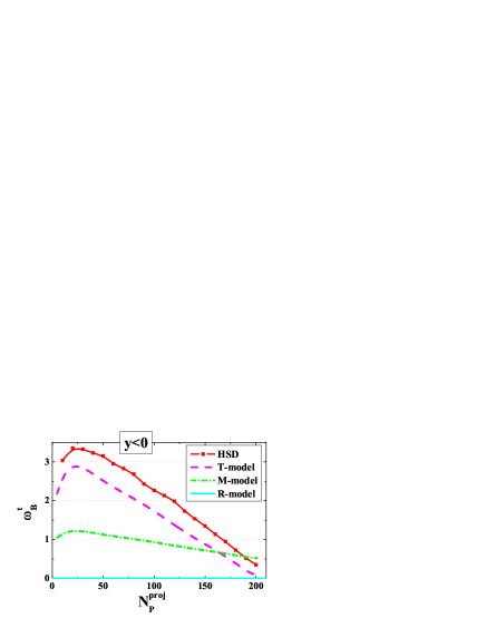
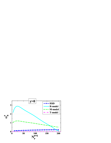
Figure 4: The $\omega_{B}^{t}$ (left) and $\omega_{B}^{p}$ (right) of the HSD simulations in comparison to T-, M- and R-models (5-7), with $\omega_{P}^{targ}$ taken from Fig. 1.

From Fig. 4 one concludes that the HSD results are close to the T-model estimates for baryon flow. However, the deviations from the results (5) are clearly seen: $\omega_{B}^{p}>0$ and $\omega_{B}^{t}>\omega_{P}^{targ}$. One can not fit the HSD values of $\omega_{B}^{t}$ and $\omega_{B}^{p}$ by Eq. (4). To make $\omega_{B}^{p}>0$ one needs $\alpha>0$, but this induces $\omega_{B}^{t}<\omega_{P}^{targ}$, i.e. a mixing of baryons between the projectile and target hemispheres creates a non-zero baryon number fluctuations in the projectile hemisphere on the expense of fluctuations in the target hemisphere. Indeed, it follows from Eq. (4) that $\omega_{B}^{p}$ increases with $\alpha$ for all $\alpha$, if $\omega_{P}^{targ}>1$, and for $\alpha<(2-\omega_{P}^{targ})^{-1}$, if $\omega_{P}^{targ}<1$. On the other hand, $\omega_{B}^{t}$ increases with $\alpha$ if $\alpha<(1-\omega_{P}^{targ})(2-\omega_{P}^{targ})^{-1}$. This shows that an increase of $\omega_{B}^{t}$ with $\alpha$ is only possible for $\omega_{P}^{targ}<1$. Thus for $\omega_{P}^{targ}>1$ one finds an increase of $\omega_{B}^{p}$ with $\alpha$ and a decrease of $\omega_{B}^{t}$ with $\alpha$ for all physical values of $\alpha$ from 0 to 1. Therefore, we conclude that the HSD values of $\omega_{B}^{t}$ (i.e. the fact that $\omega_{B}^{t}>\omega_{P}^{targ}$) can not be explained by Eq. (4) with $\alpha>0$.

The numbers of target and projectile participants are defined as $N_{P}^{targ}\equiv A-N_{S}^{targ}$ and $N_{P}^{proj}\equiv A-N_{S}^{proj}$. The actual event-by-event numbers of baryons in the target and projectile hemispheres, $N_{B}^{t}$ and $N_{B}^{p}$, may differ from $N_{P}^{targ}$ and $N_{P}^{proj}$. This is because a transfer of baryons between the projectile and target hemispheres arises from the production of baryon-antibaryon pairs. The partners of each newly created $b\overline{b}$-pair can be detected with non-zero probability in different hemispheres. We introduce $b^{t}\equiv N_{B}^{t}-N_{P}^{targ}$ and the number of antibaryons in the target hemisphere, $\overline{b}^{t}$. Similarly, $b^{p}\equiv N_{B}^{p}-N_{P}^{proj}$, while $\overline{b}^{p}$ is the number of antibaryons in the projectile hemisphere. One finds:

$$\omega_{B}^{t}~{}\equiv\frac{Var(N_{P}^{targ}~{}+~{}b^{t}~{}-~{}\overline{b}^{t})}{\langle B^{t}\rangle}~{}=~{}\omega_{P}^{targ}~{}$$

$$+~{}\frac{1}{N_{P}^{proj}}~{}\left[Var(b^{t})~{}+~{}Var(\overline{b}^{t})~{}+~{}2~{}\Delta(N_{P}^{targ},~{}b^{t})~{}-~{}2~{}\Delta(N_{P}^{targ},~{}\overline{b}^{t})~{}-~{}2~{}\Delta(b^{t},~{}\overline{b}^{t})~{}\right]~{},$$ (8)

$$\omega_{B}^{p}~{}\equiv\frac{Var(N_{P}^{proj}~{}+~{}b^{p}~{}-~{}\overline{b}^{p})}{\langle B^{p}\rangle}~{}=~{}\frac{1}{N_{P}^{proj}}~{}\left[Var(b^{p})~{}+~{}Var(\overline{b}^{p})~{}-~{}2~{}\Delta(b^{p},~{}\overline{b}^{p})~{}\right]~{},$$ (9)

where

$$\Delta(N_{1},~{}N_{2})~{}\equiv~{}\langle N_{1}~{}\cdot~{}N_{2}\rangle~{}-~{}\langle N_{1}\rangle~{}\cdot~{}\langle N_{2}\rangle~{}.$$ (10)

As $N_{P}^{proj}=const$ in the sample, it follows that $\omega_{P}^{proj}=0$, $\Delta(N_{P}^{proj},~{}b^{p})=0$, $\Delta(N_{P}^{proj},~{}\overline{b}^{p})=0$, these terms are absent in the r.h.s. of Eq. (9). Different terms of Eq. (8) and Eq. (9) found from the HSD simulations are presented in Fig 5.

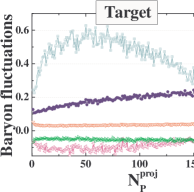
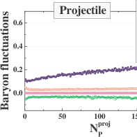
Figure 5: Different terms of Eq. (8), left, and Eq. (9), right, are presented as a function of $N_{P}^{proj}$.

One observes that terms of Eq. (8,9) expressing the fluctuations of antibaryons, $Var(\overline{b}^{p})/N_{P}^{proj}$, and the correlation terms, $2\Delta(N_{P}^{targ},~{}\overline{b}^{t})/N_{P}^{proj}$ and $~{}-~{}2\Delta(b^{t},~{}\overline{b}^{t})/N_{P}^{proj}$, with antibaryons included, are small. Therefore, one finds, $\omega_{B}^{p}\cong Var(b^{p})/N_{P}^{proj}$. In the target hemisphere, the $\omega_{P}^{targ}$ gives the main contribution to $\omega_{B}^{t}$ in Eq. (8). The term $Var(b^{t})/N_{P}^{proj}$ also contributes to $\omega_{B}^{t}$, similarly to that, $Var(b^{p})/N_{P}^{proj}$, in the projectile hemisphere. However, the main additional term to $\omega_{B}^{t}$ is $2\Delta(N_{P}^{targ},~{}b^{t})/N_{P}^{proj}$, which is due to (positive) correlations between $N_{P}^{targ}$ and $b^{t}$. This implies that in events with large $N_{P}^{targ}$ (i.e. $N_{P}^{targ}>\langle N_{P}^{targ}\rangle\cong N_{P}^{proj}$) some additional baryons move from the projectile to the target hemisphere, and when $N_{P}^{targ}$ is small (i.e. $N_{P}^{targ}<\langle N_{P}^{targ}\rangle\cong N_{P}^{proj}$) the baryons move in the reverse direction from the target to the projectile hemisphere as shown in Fig. 6.

Figure 6: The HSD results for Pb+Pb collisions at 158 AGeV for the rapidity distributions of baryon numbers in nonsymmetric samples with $N_{P}^{proj}=50,N_{P}^{targ}=78$ (left), and $N_{P}^{proj}=50,N_{P}^{targ}=20$ (right).

This HSD result looks rather unexpected. We remind that Eq. (4) predicts for $\omega_{B}^{t}$ the opposite behavior: due to a simple mixing of baryons between the target and projectile hemispheres the initially large fluctuations, $\omega_{P}^{targ}$, are transformed into smaller ones, $\omega_{B}^{t}$. It seems that the origin of this effect is the following: For $N_{P}^{targ}>N_{P}^{proj}$ each projectile nucleon interacts, in average, more often than the target nucleon. The projectile participant loses then a larger part of its energy, and in the rapidity space its position becomes closer to $y_{c.m.}=0$ than the position of target participants. This gives to projectile participants more chances to move due to further rescatterings from projectile to target hemisphere, in a comparison with target participants to move in the opposite direction. For $N_{P}^{targ}<N_{P}^{proj}$ there is a reverse situation. This fact was not taken into account in Eqs. (2,3) where it has been assumed that the mixing probability $\alpha$ is the same for projectile and target participants, and independent of $N_{P}^{targ}$.

IV Net Electric Charge Fluctuations

The T-, M- and R-models give very different predictions for $\omega_{B}^{p}$ and $\omega_{B}^{t}$ for the samples of events with fixed values of $N_{P}^{targ}$. Additional interesting correlations between the $B^{t}$ and $B^{p}$ numbers, as those seen in the HSD simulations, can be expected. Unfortunately, they may be difficult to test experimentally as an identification of protons and a measurement of neutrons in a large acceptance in a single event is difficult. Measurements of the charged particle multiplicity in a large acceptance can be performed with the existing detectors. In this section we consider the HSD results for the net electric charge, $Q$, fluctuations. As $Q\cong 0.4B$ in the initial heavy nuclei one can naively expect that $Q$ fluctuations are quite similar to $B$ fluctuations. We stress, however, a principal difference between $Q$ and $B$ in relativistic A+A collisions. Fig. 7 demonstrates the rapidity distributions of the net baryon number, $B=N_{B}-N_{\overline{B}}$  (left), and total number of baryons, $N_{B}+N_{\overline{B}}$  (right), for different centralities in Pb+Pb collisions at 158 AGeV. One observes that both quantities are very close to each other; the $y$-dependence and absolute values are very close for $B$ and $N_{B}-N_{\overline{B}}$ distributions. This is, of course, because the number of antibaryons is rather small, $N_{\overline{B}}\ll N_{B}$.

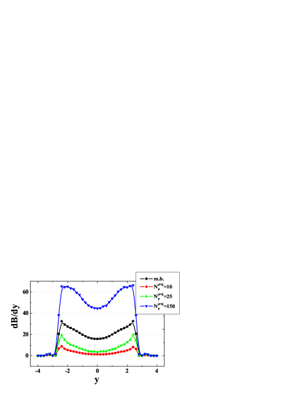
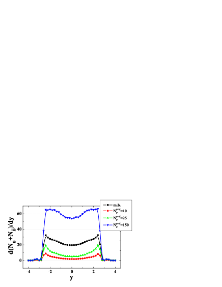
Figure 7: The HSD rapidity distributions in Pb+Pb collisions at 158 AGeV for the net baryon number, $B=N_{B}-N_{\overline{B}}$ (left), and total number of baryons, $N_{B}+N_{\overline{B}}$ (right), at different $N_{P}^{proj}$ and in the minimum bias (m.b.) sample.

Fig. 8 shows the same as Fig. 7 but for the electric charge $Q=N_{+}-N_{-}$  (left), and total number of charged particles, $N_{ch}\equiv N_{+}+N_{-}$  (right).

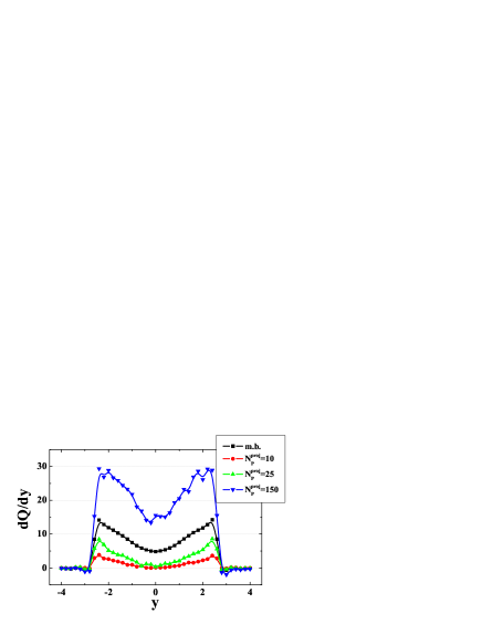
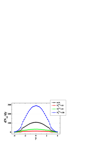
Figure 8: The same as in Fig. 7 but for the electric charge $Q=N_{+}-N_{-}$  (left), and total number of charged particles, $N_{ch}\equiv N_{+}+N_{-}$  (right).

The $y$-dependence of $dQ/dy$ and $dN_{ch}/dy$ is quite different. Besides, the absolute values of $N_{ch}$ are about 10 times larger than those of $Q$. This implies that $Q\ll N_{+}\approx N_{-}$.

In the previous section we have used the scaled variance $\omega_{B}$ to quantify the measure of the net baryon fluctuations. It appears to be a useful variable as $\omega_{B}$ is straightforwardly connected to $\omega_{P}^{targ}$ and due to the relatively small number of antibaryons. Fig. 8 tells that $\omega_{Q}$ is a bad measure of the electric charge fluctuations in high energy A+A collisions. One observes that $\omega_{Q}\equiv Var(Q)/\langle Q\rangle$ is much larger than 1 simply due to the small value of $\langle Q\rangle$ in a comparison with $N_{+}$ and $N_{-}$. If the A+A collision energy increases, it follows, $\langle Q\rangle\rightarrow 0$, and thus $\omega_{Q}\rightarrow\infty$. The same will happen with $\omega_{B}$, too, at much larger energies. A useful measure of the net electric charge fluctuations is the quantity (see, e.g., fluc7a ):

$$X_{Q}~{}\equiv~{}\frac{Var(Q)}{\langle N_{ch}\rangle}~{}.$$ (11)

A value of $X_{Q}$ can be easily calculated for the Boltzmann ideal gas in the grand canonical ensemble. In this case the number of negative and positive particles fluctuates according to the Poisson distribution (i.e. $\omega_{-}=\omega_{+}=1$), and the correlation between $N_{+}$ and $N_{-}$ are absent (i.e. $\langle N_{+}N_{-}\rangle=\langle N_{+}\rangle\langle N_{-}\rangle$), so that $X_{Q}=1$. On the other hand, the canonical ensemble formulation (i.e. when $Q=const$ fixed exactly for all microscopic states of the system) leads to $X_{Q}=0$. Fig. 9 shows the results of the HSD simulations for the full acceptance, for the projectile and target hemispheres (left), and also for symmetric rapidity intervals in the c.m.s. (right).

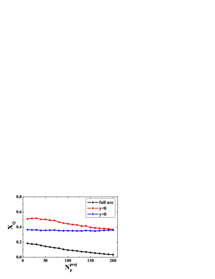
Figure 9: Left: The HSD simulations in Pb+Pb collisions at 158 AGeV for $X_{Q}$ at different values of $N_{P}^{proj}$ in the full acceptance (lower curve), for the projectile (middle curve) and target (upper curve) hemispheres. Right: The same, but for symmetric rapidity intervals in the c.m.s.

The $Q$ fluctuation in the full acceptance is due to $N_{P}^{targ}$ fluctuations. As $Q\cong 0.4B$ in colliding (heavy) nuclei, one may expect $Var(Q)\cong 0.16~{}Var(B)$. In addition, $\langle N_{ch}\rangle\cong 4\langle N_{P}\rangle$ at 158 AGeV, so that one estimates $X_{Q}\cong 0.04~{}\omega_{B}$ for the fluctuations in the full phase space. The actual values of $X_{Q}$ presented in Fig. 9 (left) are about 3 times larger. This is because of $Q$ fluctuations due to different event-by-event values of proton and neutron participants even in a sample with fixed values of $N_{P}^{proj}$ and $N_{P}^{targ}$.

From Fig. 9 (right) one sees only a tiny difference between the $X_{Q}$ values in the symmetric rapidity intervals in the projectile and target hemispheres, and slightly stronger effects for the whole projectile and target hemispheres (Fig. 9, right). In fact, the fluctuations of $N_{+}$ and $N_{-}$ are very different in the projectile and target hemispheres, and the scaled variances $\omega_{+}^{t}$ and $\omega_{-}^{t}$ have a very strong $N_{P}^{proj}$-dependence. This is shown in Fig. 10 obtained in our previous study KGB .

Figure 10: The HSD results for the scaled variances of negatively (left) and positively (right) charged hadrons in Pb+Pb collisions at 158 AGeV for the projectile (lower curves) and target (upper curves) hemispheres.

The $X_{Q}$ can be presented in two equivalent forms

$$X_{Q}~{}=~{}\omega_{+}~{}\frac{\langle N_{+}\rangle}{\langle N_{ch}\rangle}~{}+~{}\omega_{-}~{}\frac{\langle N_{-}\rangle}{\langle N_{ch}\rangle}~{}-~{}2~{}\frac{\Delta(N_{+},N_{-})}{\langle N_{ch}\rangle}~{}=~{}2~{}\omega_{+}~{}\frac{\langle N_{+}\rangle}{\langle N_{ch}\rangle}~{}+~{}2~{}\omega_{-}~{}\frac{\langle N_{-}\rangle}{\langle N_{ch}\rangle}~{}-~{}\omega_{ch}~{}.$$ (12)

Eq. (12) is valid for any region of the phase space: full phase space, projectile or target hemisphere, etc. As seen from Fig. 10, both $\omega_{+}^{t}$ and $\omega_{-}^{t}$ are large and strongly $N_{P}^{proj}$-dependent. This is not seen in $X_{Q}^{t}$ because of strong correlations between $N_{+}^{t}$ and $N_{-}^{t}$, i.e. the term $2~{}\Delta(N_{+},N_{-})/\langle N_{ch}\rangle$ compensates $\omega_{+}$ and $\omega_{-}$ terms in Eq. (12). This is also seen from Fig. 11.

Figure 11: The HSD results for the scaled variances of all charged hadrons, $\omega_{ch}$, in Pb+Pb collisions at 158 AGeV for the projectile (lower curve) and target (upper curve) hemispheres.

A cancellation of strong $N_{P}^{proj}$-dependence in the target hemisphere takes place between the sum of $\omega_{+}^{t}$ and $\omega_{-}^{t}$ terms of Eq. (12), and the $~{}\omega_{ch}^{t}$-term.

Fig. 12 shows a comparison of the HSD results for $X_{Q}$ with NA49 data in Pb+Pb collisions at 158 AGeV for the forward rapidity interval $1.1<y<2.6$ inside the projectile hemisphere with additional $p_{T}$-filter imposed.

Figure 12: The HSD results for $X_{Q}$ for Pb+Pb collisions at 158 AGeV for the forward rapidity interval $1.1<y<2.6$ inside the projectile hemisphere. The solid dots are the estimates obtained from Eq. (12) using the NA49 experimental data NA49 (the errorbars are not indicated here). For illustration, the HSD results in the symmetric backward rapidity interval $-2.6<y<-1.1$ (target hemisphere) are also presented.

As an illustration, the HSD results in the symmetric backward rapidity interval $-2.6<y<-1.1$ (target hemisphere) are also included. One observes no difference between the $X_{Q}$ results for the NA49 acceptance in the projectile and target hemispheres. The HSD values for $\omega_{+}$, $\omega_{-}$, and $\omega_{ch}$ are rather different in the projectile and target hemispheres for the NA49 acceptance (see Figs. 10 and 11). This is not seen in Fig. 12 for $X_{Q}$. As explained above a cancellation between $\omega_{+}$, $\omega_{-}$ and $\omega_{ch}$ terms take place in Eq. (12). In fact, NA49 did not perform the $X_{Q}$ measurements. The $X_{Q}$-data (solid dots) presented in Fig. 12 are obtained from Eq. (12) using the NA49 data for $\omega_{+}$, $\omega_{-}$, and $\omega_{ch}$ as well as $\langle N_{+}\rangle$, $\langle N_{-}\rangle$, and $\langle N_{ch}\rangle$ NA49 . Such a procedure leads, however, to very large errors for $X_{Q}$ (which are not indicated in Fig. 12) which excludes any conclusion about the (dis)agreement of HSD results with NA49 data.

V Fluctuations in Most Central Collisions

In this section we consider the baryon number and electric charge fluctuations in the symmetric rapidity interval $[-y,y]$ in the c.m.s. for the most central Pb+Pb events. We chose the sample of most central events by restricting the impact parameter to $b<2$ fm. It gives about 2% most central Pb+Pb collisions from the whole minimum bias sample. Fig. 13 shows the HSD results for electric charge fluctuations in 2% most central Pb+Pb collisions for the symmetric rapidity interval $\Delta Y=[-y,y]$ in the c.m.s. as the function of $\Delta y=\Delta Y/2$.

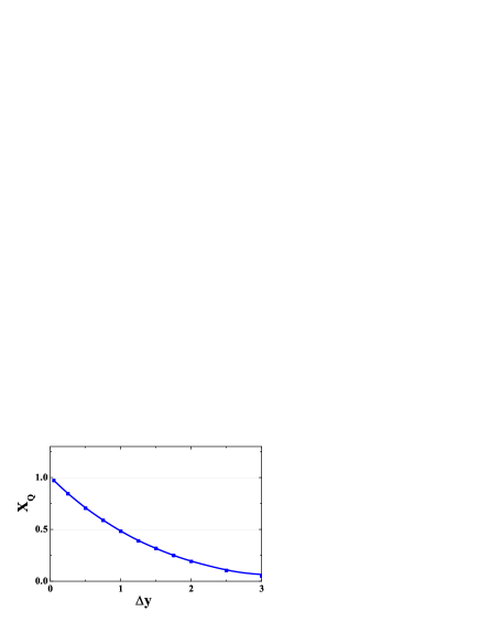
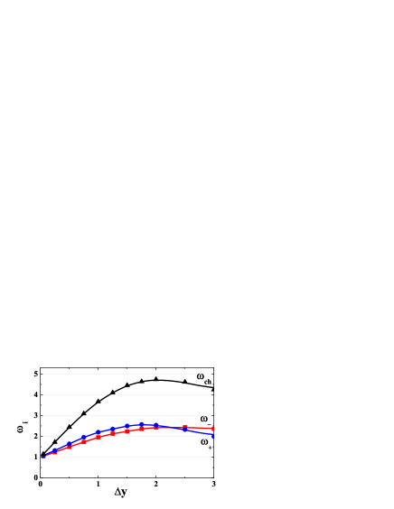
Figure 13: The HSD results for electric charge fluctuations in 2% most central Pb+Pb collisions at 158 AGeV in the symmetric rapidity interval , $\Delta Y=[-y,y]$ as a function of $\Delta y=\Delta Y/2$ in the c.m.s. A left panel shows the behavior of $X_{Q}$, and a right one demonstrates separately $\omega_{+}$, $\omega_{-}$, and $\omega_{ch}$.

For $\Delta Y\rightarrow 0$ one finds $X_{Q}\rightarrow 1$. This can be understood as follows: For $\Delta Y\rightarrow 0$ the fluctuations of negatively, positively and all charged particles behave as for the Poisson distribution: $\omega_{+}\cong\omega_{-}\cong\omega_{ch}\cong 1$. Then from Eq. (12) it follows that $X_{Q}\cong 1$, too. From Fig. 13 (right) one observes that $\omega_{+}$, $\omega_{-}$, and $\omega_{ch}$ all increase with increasing interval $\Delta Y$. However, $X_{Q}$ decreases with $\Delta Y$ and – because of global $Q$ conservation – it goes approximately to zero when all final particles are accepted.

In Fig. 14 (left) the HSD results for the scaled variances are presented in full acceptance as functions of $N_{P}^{proj}$. Fig.14 (right) demonstrates the probability distribution of events with $b<2$ fm over $N_{P}^{proj}$.

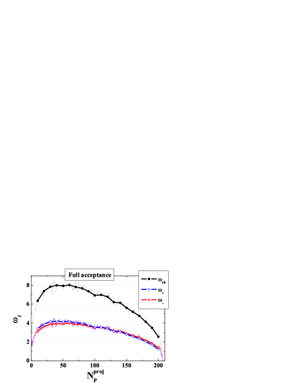
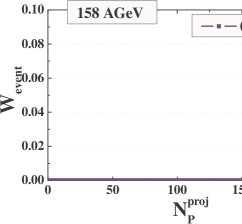
a

Figure 14: The HSD results in Pb+Pb collisions at 158 AGeV. Left: The scaled variances $\omega_{+}$, $\omega_{-}$, and $\omega_{ch}$ in the full acceptance. Right: The distributions of events over $N_{P}^{proj}$ in most central collisions with $b<2$ fm.

One observes that even in the 2% centrality sample the values of $N_{P}^{proj}$ are noticeably smaller than the maximum value, $A=208$. As seen from Fig. 14 (left) the HSD values of $\omega_{+}$, $\omega_{-}$, and $\omega_{ch}$ become then essentially larger than 1 in agreement with those presented in Fig. 13.

Fig. 15 shows the net baryon number fluctuations in the symmetric rapidity interval $[-y,y]$ in the c.m.s. as the function of $\Delta Y$.

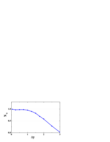
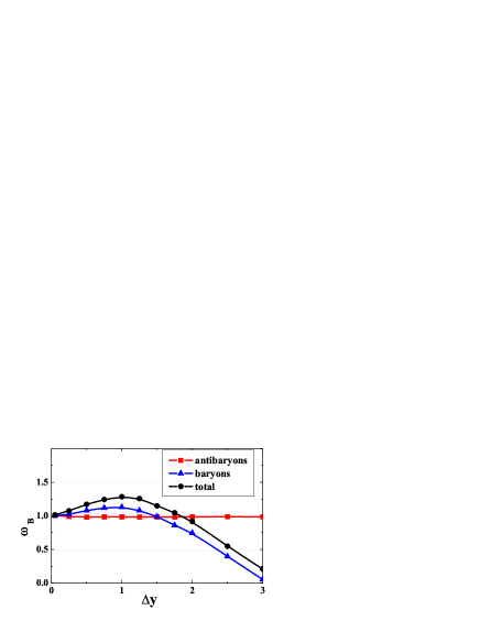
Figure 15: The HSD results for net baryon number fluctuations in 2% most central Pb+Pb collisions at 158 AGeV in the symmetric rapidity interval $\Delta Y=[-y,y]$ as a function of $\Delta y=\Delta Y/2$ in the c.m.s. The left panel shows the behavior of $X_{B}$, and a right panel presents separately $\omega_{N_{B}}$, $\omega_{N_{\overline{B}}}$, and $\omega_{N_{B}+N_{\overline{B}}}$.

As a measure of the net baryon number fluctuations we have used the quantity,

$$X_{B}~{}\equiv~{}\frac{Var(B)}{\langle N_{B}~{}+~{}N_{\overline{B}}\rangle}~{}.$$ (13)

As for the electric charge, one finds that $X_{B}\rightarrow 1$ at $\Delta Y\rightarrow 0$ (this is because all $\omega_{N_{B}}$, $\omega_{N_{\overline{B}}}$, and $\omega_{N_{B}+N_{\overline{B}}}$ go to 1 in this limit (see Fig. 15, left), and $X_{B}\rightarrow 0$ at upper limit of $\Delta Y$ because of global baryon number conservation.

Writing the variance $Var(B)$ in the form,

$$Var(B)~{}=2~{}Var(N_{B})~{}+~{}2~{}Var(N_{\overline{B}})~{}-~{}Var(N_{B}~{}+~{}N_{\overline{B}})~{},$$ (14)

we find

$$X_{B}~{}=~{}2~{}\omega_{N_{B}}~{}\frac{\langle N_{B}\rangle}{\langle N_{B}~{}+~{}N_{\overline{B}\rangle}}~{}+~{}2~{}\omega_{N_{\overline{B}}}~{}\frac{\langle N_{\overline{B}}\rangle}{\langle N_{B}~{}+~{}N_{\overline{B}}\rangle}~{}-~{}~{}\omega_{N_{B}+N_{\overline{B}}}.$$ (15)

The behavior of the different terms in Eq. (15) is the following: As seen from Fig. 15, right, $\omega_{N_{\overline{B}}}\cong 1$ for all values of $\Delta Y$. This is because $N_{\overline{B}}\ll N_{B}$, and baryon number conservation does not affect the fluctuations of antibaryons. Due to the small number of antibaryons in comparison to baryons, one also observes $\omega_{B}\cong\omega_{N_{B}}\cong\omega_{N_{B}+N_{\overline{B}}}$.

VI Electric charge fluctuations in central Pb+Pb collisions at 20, 30, 40, 80 and 160 A GeV

In this section we present the HSD results for the event-by-event electric charge fluctuations as measured by the NA49 Collaboration in central Pb+Pb collisions at 20, 30, 40, 80 and 160 A GeV exFq_NA49 . The interest in this observable (as a signal of deconfinement) is related to the predicted in Refs.Ko.1 ; As.1 suppression of event-by-event fluctuations of the electric charge in a quark-gluon plasma relative to a hadron gas. However, these predictions were based on the assumption that the initial electric charge fluctuations survive the hadronization phase.

The first experimental measurement of charge fluctuations in central heavy-ion collisions by PHENIX Adcox:2002mm and STAR Adams:2003st at RHIC and by the NA49 exFq_NA49 at SPS showed a quite moderate suppression of the electric charge fluctuations. This observation has been attributed to the fact that the initial fluctuations are distorted by the hadronization. In particular, the observed fluctuations might be related to the final resonance decays.

In this respect it is important to compare the experimental data with the results of microscopic transport models such as HSD where the resonance decays are included by default. In order to quantify the event-by-event electric charge fluctuations we have calculated the quantity $\Phi$ defined as exFq_NA49 ; Ma.1 :

$$\Phi_{q}=\sqrt{\frac{\langle Z^{2}\rangle}{\langle N\rangle}}-\sqrt{\overline{z^{2}}}\;,$$ (16)

where

$$z=q-\overline{q},\;\;\;\;\;\;\;\;Z=\sum_{i=1}^{N}(q_{i}-\overline{q}).$$ (17)

Here $q$ denotes a single particle variable, i.e. electric charge $q$; $N$ is the number of particles of the event within the acceptance, and over-line and $\langle...\rangle$ denote averaging over a single particle inclusive distribution and over events, respectively. By construction, $\Phi$ of the system, which is an independent sum of identical sources of particles, is equal to the $\Phi$ for a single source Ma.1 ; Ma.2 .

In order to remove the sensitivity of the final signal to the trivial global charge conservation (GCC) the measure $\Delta\Phi_{q}$ is defined as the difference:

$$\Delta\Phi_{q}=\Phi_{q}-\Phi_{q,\rm{GCC}}\;.$$ (18)

Here the value of $\Phi_{q}$ is given by Za.1 ; Mrowczynski:2001mm :

$$\Phi_{q,\rm{GCC}}=\sqrt{1-P}-1,$$ (19)

where

$$P=\frac{\langle N_{ch}\rangle}{\langle N_{ch}\rangle_{tot}}$$ (20)

with $\langle N_{ch}\rangle$ and $\langle N_{ch}\rangle_{tot}$ being the mean charged multiplicity in the detector acceptance and in full phase space (excluding spectator nucleons), respectively.

By construction, the value of $\Delta\Phi_{q}$ is zero if the particles are correlated by global charge conservation only. It is negative in case of an additional correlation between positively and negatively charged particles, and it is positive if the positive and negative particles are anti-correlated Za.1 .

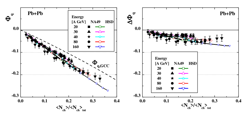
Figure 16: The dependence of the $\Phi_{q}$ (l.h.s.) and $\Delta\Phi_{q}$ (r.h.s.) on the fraction of accepted particles for central Pb+Pb collisions at 20-158 AGeV. The NA49 data exFq_NA49 are shown as full symbols, whereas the open symbols (connected by lines) stay for the HSD results. The dashed line shows the dependence expected for the case if the only source of particle correlations is the global charge conservation $\Phi_{q,GCC}$, Eq. 19.

Figure 16 shows the HSD results for the dependence of $\Phi_{q}$ (l.h.s.) and $\Delta\Phi_{q}$ (r.h.s.) on the fraction of accepted particles $\langle N_{ch}\rangle$ and $\langle N_{ch}\rangle_{tot}$ (calculated for ten different rapidity intervals increasing in size from $\Delta y=0.3$ to $\Delta y=3$ in equal steps) for central Pb+Pb collisions at 20, 30, 40, 80 and 158 A GeV. The NA49 data exFq_NA49 are shown as full symbols, whereas the open symbols (connected by lines) reflect the HSD results. The dashed line shows the dependence expected for the case if the only source of particle correlations is the global charge conservation $\Phi_{q,GCC}$ (Eq. (19)).

The data as well as the HSD results for $\Phi_{q}$ (Fig. 16, l.h.s.) are in a good agreement and show a monotonic decrease with increasing fraction of accepted particles. After substraction the contribution by global charge conservation (the dashed line in Fig. 16), the values of $\Delta\Phi_{q}$ vary between $0$ and $-0.05$ which are significantly larger than the values expected for QGP fluctuations ($-0.5<\Delta\Phi_{q}<-0.15$ Za.1 ).

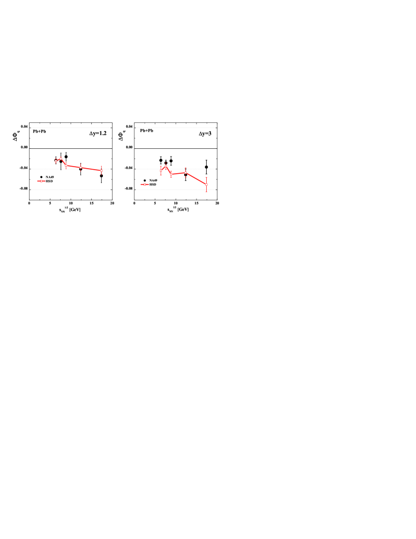
Figure 17: The energy dependence of $\Delta\Phi_{q}$ measured in central Pb+Pb collisions for a narrow rapidity interval $\Delta y=1.2$ (l.h.s.) and a broad rapidity interval $\Delta y=3$ (r.h.s.). The NA49 data exFq_NA49 are shown as full symbols, whereas the the open symbols (connected by lines) reflect the HSD results.

Figure 17 presents the energy dependences of $\Delta\Phi_{q}$ for two selected rapidity intervals – the intermediate rapidity interval $\Delta y=1.2$ (l.h.s.) and for the largest rapidity interval $\Delta y=3$ (r.h.s.). The both, data and HSD results, show the a weak decrease of $\Delta\Phi_{q}$ with increasing energy.

The fact that the HSD model, that includes no explicit phase transition, describes the experimental data can be considered an independent proof that the event-by-event charge fluctuations are driven by the hadronization phase and dominantly by the resonance decays (which are naturally included in HSD) and no longer sensitive to the initial phase fluctuations from a QGP.

VII Summary and conclusions

The goal of this study was to investigate the sensitivity of event-by-event fluctuations of baryon number and electric charge to the early stage dynamics of hot and dence nuclear matter created in heavy-ion collisions at SPS energies and the influance of the futher hadronization and rescattering phase. For that perpose we have explored the microscopic HSD transport model which allows also to investigate (on event-by-event basis) the influence of the experimental acceptance and the set-up on the final observables.

It has been found that the fluctuations in the number of target participants strongly influences the baryon number and charged multiplicity fluctuations. The consequences of this fact depend crucially on the dynamics of the initial flows of the conserved charges and inelastic energy.

For a better quantitative understanding of the microscopic transport model (HSD) results we have considered 3 limiting groups of models for nucleus-nucleus collisions: transparency, mixing and reflection. These ”pedagogical” considerations indicate that the HSD model (as well as UrQMD, cf. Ref. KGB ) shows only a small mixing on initial baryon flow and is closer to the T-model. This supports the findings from Ref. Weber about the influence of the partonic degrees of freedom on the initial phase dynamics which might increase the mixing by additional strong parton-parton interactions. Thus, the measurement of the net baryon number fluctuations helps to quantify the mixing of initial baryon flow.

The first microscopic event-by-event calculations of the charge fluctuations $\Delta\Phi_{q}$ within the HSD model show a good agreement with the NA49 data at SPS energies. Thus, this observable is dominated by the final stage danymics, i.e. the hadronization phase and the resonance decays, and rather insensitive to the initial QGP dynamics.

- (1) W. Ehehalt and W. Cassing, Nucl. Phys. A 602, 449 (1996); W. Cassing and E.L. Bratkovskaya, Phys. Rep. 308, 65 (1999); W. Cassing, E. L. Bratkovskaya, and A. Sibirtsev, Nucl. Phys. A 691, 753 (2001).
- (2) H. Weber, E. L. Bratkovskaya, W. Cassing, and H. Stöcker, Phys. Rev. C67, 014904 (2003); E. L. Bratkovskaya, M. Bleicher, M. Reiter, S. Soff, H. Stöcker, M. van Leeuwen, S. A. Bass, and W. Cassing, Phys. Rev. C69, 054907 (2004); E. L. Bratkovskaya, M. Bleicher, W. Cassing, M. Reiter, S. Soff, H. Stöcker, Prog. Part. Nucl. Phys. 53, 225 (2004); E. L. Bratkovskaya, W. Cassing, and H. Stöcker, Phys. Rev. C 67, 054905 (2003).
- (3) M. Gaździcki and St. Mrówczyński, Z. Phys. C 26, 127 (1992);
- (4) L. Stodolsky, Phys. Rev. Lett. 75, 1044 (1995); E.V. Shuryak, Phys. Lett. B 423, 9 (1998); St. Mrówczyński, Phys. Lett. B 430, 9 (1998).
- (5) G. Baym and H. Heiselberg, Phys. Lett. B 469, 7 (1999).
- (6) I.N. Mishustin, Phys. Rev. Lett. 82, 4779 (1999); Nucl. Phys. A 681, 56c (2001); H. Heiselberg and A.D. Jackson, Phys. Rev. C 63, 064904 (2001).
- (7) M.A. Stephanov, K. Rajagopal, and E.V. Shuryak, Phys. Rev. Lett. 81, 4816 (1998); Phys. Rev. D 60, 114028 (1999); M.A. Stephanov, Acta Phys. Polon. B 35, 2939 (2004).
- (8) S. Jeon and V. Koch, Phys. Rev. Lett. 83, 5435 (1999); ibid. 85, 2076 (2000).
- (9) H. Heiselberg, Phys. Rep. 351, 161 (2001).
- (10) S. Jeon and V. Koch, hep-ph/0304012, Review for Quark-Gluon Plasma 3, eds. R.C. Hwa and X.-N. Wang, World Scientific, Singapore.
- (11) M. Bleicher et al., Nucl. Phys. A 638, 391 (1998); Phys. Lett. B 435, 9 (1998); Phys. Rev. C 62, 061902 (2000); ibid. 62, 041901 (2000); S. Jeon, L. Shi, and M. Bleicher, Phys. Rev. C 73, 014905 (2006). S. Haussler, H. Stoecker, and M. Bleicher, Phys. Rev. C 73, 021901 (2006).
- (12) M. Gaździcki, M.I. Gorenstein, and St. Mrówczyński, Phys. Lett. B 585, 115 (2004); M.I. Gorenstein, M. Gaździcki, and O.S. Zozulya, ibid. 585, 237 (2004); M. Gaździcki, J. Phys. Conf. Ser. 27, 154 (2005), nucl-ex/0507017.
- (13) H. Stöcker and W. Greiner, Phys. Rep. 137, 277 (1986); J. Cleymans and H. Satz, Z. Phys. C 57, 135 (1993); J. Sollfrank, M. Gaździcki, U. Heinz, and J. Rafelski, ibid. 61, 659 (1994); G.D. Yen, M.I. Gorenstein, W. Greiner, and S.N. Yang, Phys. Rev. C 56, 2210 (1997); F. Becattini, M. Gaździcki, and J. Solfrank, Eur. Phys. J. C 5, 143 (1998); G.D. Yen and M.I. Gorenstein, Phys. Rev. C 59, 2788 (1999); P. Braun-Munzinger, I. Heppe and J. Stachel, Phys. Lett. B 465, 15 (1999); P. Braun-Munzinger, D. Magestro, K. Redlich, and J. Stachel, ibid. 518, 41(2001); F. Becattini, M. Gaździcki, A. Keränen, J. Mannienen, and R. Stock, Phys. Rev. C 69, 024905 (2004).
- (14) P. Braun-Munzinger, K. Redlich, J. Stachel, nucl-th/0304013, Review for Quark Gluon Plasma 3, eds. R.C. Hwa and X.-N. Wang, World Scientific, Singapore.
- (15) F. Becattini, Z. Phys. C 69, 485 (1996); F. Becattini, U. Heinz, ibid. 76, 269 (1997); F. Becattini, G. Passaleva, Eur. Phys. J. C 23, 551 (2002).
- (16) V.V. Begun, M. Gaździcki, M.I. Gorenstein, and O.S. Zozulya, Phys. Rev. C 70, 034901 (2004); V.V. Begun, M.I. Gorenstein, and O.S. Zozulya, Phys. Rev. C 72, 014902 (2005); A. Keränen, F. Becattini, V.V. Begun, M.I. Gorenstein, and O.S. Zozulya, J. Phys. G 31, S1095 (2005); F. Becattini, A. Keranen, L. Ferroni, T. Gabbriellini, Phys. Rev. C 72, 064904 (2005); V.V. Begun, M.I. Gorenstein, A.P. Kostyuk, and O.S. Zozulya, Phys. Rev. C 71, 054904 (2005); J. Cleymans, K. Redlich, L. Turko, Phys. Rev. C 71, 047902 (2005); J. Cleymans, K. Redlich, L. Turko, J. Phys. G 31, 1421-1435 (2005); V.V. Begun, M.I. Gorenstein, A.P. Kostyuk, and O.S. Zozulya, J. Phys. G 32, 935 (2006). V.V. Begun and M.I. Gorenstein, Phys. Rev. C 73, 054904 (2006).
- (17) V.P. Konchakovski, S. Haussler, M.I. Gorenstein, E.L. Bratkovskaya, M. Bleicher, and H. Stöcker, Phys. Rev. C 73, 034902 (2006).
- (18) M. Gaździcki and M.I. Gorenstein, Phys. Lett. B 640, 155 (2006).
- (19) U. Katscher, D. H. Rischke, J. A. Maruhn, W. Greiner, I. N. Mishustin and L. M. Satarov, Z. Phys. A 346, 209 (1993), Yu. B. Ivanov, V.N. Russkikh and V. D. Toneev, Phys. Rev. C 73, 044904 (2006).
- (20) M. Rybczynski et al. [NA49 Collaboration], J. Phys. Conf. Ser. 5, 74 (2005); T. Anticic et al. [NA49 Collaboration], Phys. Rev. C 70, 034902 (2004); P. Dinkelaker [NA49 Collaboration], J. Phys. G 31, S1131 (2005).
- (21) A. Bialas and W. Czyz, Acta Phys. Polon. B 36, 905 (2005).
- (22) C. Alt et al. [NA49 Collaboration], Phys. Rev. C 70 (2004) 064903.
- (23) S. Jeon and V. Koch, Phys. Rev. Lett. 85, 2076 (2000).
- (24) M. Asakawa, U. W. Heinz and B. Muller, Phys. Rev. Lett. 85, 2072 (2000).
- (25) K. Adcox et al. [PHENIX Collaboration], Phys. Rev. Lett. 89, 082301 (2002).
- (26) J. Adams et al. [STAR Collaboration], Phys. Rev. C 68, 044905 (2003).
- (27) M. Gazdzicki and S. Mrowczynski, Z. Phys. C 54, 127 (1992).
- (28) M. Gazdzicki, Eur. Phys. J. C 8, 131 (1999).
- (29) S. Mrowczynski, Phys. Rev. C 66, 024904 (2002).
- (30) J. Zaranek, Phys. Rev. C 66, 024905 (2002).