Time-odd triaxial relativistic mean field approach for nuclear magnetic moment

Abstract

The time-odd triaxial relativistic mean field approach is developed and applied to the investigation of the ground-state properties of light odd-mass nuclei near the double-closed shells. The nuclear magnetic moments including the isoscalar and isovector ones are calculated and good agreement with Schmidt values is obtained. Taking ¹⁷F as an example, the splitting of the single particle levels ( around $~{}0.7$ MeV near the Fermi level ), the nuclear current, the core polarizations, and the nuclear magnetic potential, i.e., the spatial part of the vector potential, due to the violation of the time reversal invariance are investigated in detail.

I Introduction

Nuclear magnetic moment is one of the most important physics observables. It provides a highly sensitive probe of the single particle structure, serves as a stringent test of the nuclear models, and has attracted the attention of nuclear physicists since the early daysStoyle56 ; Wildenthal79 ; Arima84 . Up to now, the static magnetic dipole moments of ground states and excited states of atomic nuclei throughout the periodic table have already been measured with several methods Stone01 . With the development of the radioactive ion beams (RIB) technique, it is now even possible to measure the nuclear magnetic moments of many short-lived nuclei near the proton and neutron drip lines with high precision Ueno96 .

Lots of efforts have been made to describe the nuclear magnetic moment non-relativistically or relativistically. In the non-relativistic theory, it has been pointed out early that the single-particle state of the shell model can couple to more complicated 2p-1h configurationsArima54 and there are mesons exchange corrections caused by the nuclear medium effect Chemtob69 . With modified g-factor or configuration mixing effect, non-relativistic approaches have turned out to be successful in reproducing data Wildenthal79 . Therefore the single particle picture in the mean field approach may not be expected to describe the magnetic moment wellArima87 . For LS closed shell nuclei plus or minus one nucleon, however, there is no spin-orbit partners on both sides of the Fermi surface and the magnetic moment operator can not couple to magnetic resonance Hofmann88 . Furthermore, the contributions from the pion-exchange current as well as others processes, e.g. $\Delta$-hole excitation, to iso-scalar current have turned to be very small in the first order approximation Towner83 ; Ichii87 . Therefore, the iso-scalar magnetic moments of the light nuclei near double-closed shells should be described well in single-particle picture.

In relativistic approach, the single particle wave function of nucleon is described by Dirac spinor with the large and small components, resulting in the relativistic effect in nuclear current and magnetic moment. Furthermore, as the spin-orbit coupling appears naturally in the relativistic approach, it is expected that the anomalous magnetic moment, which is related to the spin of nucleons, can be described well in relativistic approach with the free g-factor for the nucleon.

During the last two decades relativistic mean field (RMF) theory has achieved great success Serot86 ; Reinhard89 ; Ring96 ; meng05ppnp in describing many nuclear phenomena for stable nuclei, exotic nuclei meng96prl ; meng98prl , as well as supernova and neutron stars Glendenning . The RMF theory incorporates many important relativistic effects from the beginning, such as a new saturation mechanism by the relativistic quenching of the attractive scalar field, the existence of anti-particle solutions, the Lorentz covariance and special relativity which make the RMF theory more appealing for studies of high-density and high temperature nuclear matter, the origin of the pseudospin symmetry Arima69 ; Hecht69 as a relativistic symmetry Ginocchio97 ; meng98prc ; meng99prc , and spin symmetry in the anti-nucleon spectrumzhou03prl , etc. Recently, good agreements with existing data for the ground-state properties of over 7000 nuclei has been achieved in the RMF+BCS model Geng05PTP .

However, it was found out that a straightforward application of the single-particle relativistic model, where only sigma and the time-component of the vector mesons were considered, can not reproduce the experimental magnetic moments Ohtsubo73 ; Miller75 ; Bawin83 ; Bouyssy84 ; Kurasawa85 . It is attributed to the small renormalized nucleon mass ($M^{*}\sim 0.6M$) which results in the enhancement of the relativistic effect on the Dirac currentShepard88 . As an improvement, the vertex corrections have to be introduced to define effective single-particle currents in nuclei, e.g., the ”back-flow” effect in the framework of the relativistic extension of Landau’s Fermi-liquid theory McNeil86 or the RPA type summation of p-h and p-$\bar{n}$ bubbles in relativistic Hartree approximation Ichii87 ; Shepard88 .

In the widely used RMF approaches, there are only the time-even fields which are essential to physical observable. In odd-A or odd-odd nuclei, however, the Dirac current due to the unpaired valence nucleon will lead to the time-odd component of vector fields, i.e., the nuclear magnetic potential. In other words, the time-odd fields will have the same effect as the ”back-flow” effect or the RPA type summation of p-h and p-$\bar{n}$ bubbles and give rise to the core polarization which will modify the nuclear current, single-particle spin and angular momentum, giving the appropriate magnetic moments. In fact, the time-odd fields are very important for the description of the magnetic moments Hofmann88 ; Furnstahl89 , and rotating nuclei Konig93 ; Mad00 , etc.

It is thus essential to consider the spatial-component of vector fields in the framework of RMF theory to investigate the single-particle properties in odd-mass nuclei. With the time-odd nuclear magnetic potential in axial deformed RMF, the iso-scalar magnetic moment have been reproduced well Hofmann88 ; Furnstahl89 . Therefore, it is interesting to include the time-odd potential into triaxial case Meng06PRC and investigate the distribution of non-vanishing spatial-component of the $\omega$ vector meson field, nuclear current, magnetic potential and magnetic moments in nuclei with odd numbers of protons and/or neutrons. Taking ¹⁷F as an example, the density distribution, single-particle energy and its splitting due to the violation of the time reversal invariance, nuclear potential, orbital momentum, etc., will be investigated. The importance of the time-odd component in the description of the nuclear current and magnetic moment will be illustrated.

The paper is arranged as the following. In Sec.II, the time-odd triaxial RMF approach is presented in detail. The splitting due to the violation of the time reversal invariance in the single-particle energy will be estimated by reducing the Dirac equation with the time-odd nuclear magnetic potential to Schrödinger equation. The numerical details for solving the triaxial RMF equations expanded in three dimensional harmonic oscillator basis are given in Sec.III. The results and discussions are presented in Sec.IV, and a short summary is given in Sec.V.

II Time-odd triaxial relativistic mean field approach

The starting point of the RMF theory is the standard effective Lagrangian density constructed with the degrees of freedom associated with the nucleon field($\psi$), two isoscalar meson fields ($\sigma$ and $\omega$), the isovector meson field ($\rho$) and the photon field ($A$) Serot86 ; Reinhard89 ; Ring96 ; meng05ppnp :

$$\displaystyle{\cal L} = \bar{\psi}\left[i\gamma^{\mu}\partial_{\mu}-M-g_{\sigma}\sigma-g_{\omega}\gamma^{\mu}\omega_{\mu}-g_{\rho}\gamma^{\mu}\vec{\tau}\cdot\vec{\rho}_{\mu}-e\gamma^{\mu}A_{\mu}\frac{1-\tau_{3}}{2}\right]\psi$$ (1)

$$\mbox{}+\frac{1}{2}\partial_{\mu}\sigma\partial^{\mu}\sigma-\frac{1}{2}m_{\sigma}^{2}\sigma^{2}-\frac{1}{3}g_{2}\sigma^{3}-\frac{1}{4}g_{3}\sigma^{4}$$

$$\mbox{}-\frac{1}{4}\Omega_{\mu\nu}\Omega^{\mu\nu}+\frac{1}{2}m_{\omega}^{2}\omega_{\mu}\omega^{\mu}+\frac{1}{4}c_{3}(\omega_{\mu}\omega^{\mu})^{2}$$

$$\mbox{}-\frac{1}{4}\vec{R}_{\mu\nu}\vec{R}^{\mu\nu}+\frac{1}{2}m_{\rho}^{2}{\vec{\rho}}_{\mu}\cdot{\vec{\rho}}^{\mu}$$

$$\mbox{}-\frac{1}{4}F_{\mu\nu}F^{\mu\nu},$$

in which the field tensors for the vector mesons and the photon are respectively defined as,

$$\displaystyle\left\{\begin{array}[]{rcl}\Omega_{\mu\nu}&=&\partial_{\mu}\omega_{\nu}-\partial_{\nu}\omega_{\mu},\\ \vec{R}_{\mu\nu}&=&\partial_{\mu}\vec{\rho}_{\nu}-\partial_{\nu}\vec{\rho}_{\mu},\\ F_{\mu\nu}&=&\partial_{\mu}{A}_{\nu}-\partial_{\nu}{A}_{\mu}.\end{array}\right.$$ (5)

The Lagrangian (1) includes respectively the non-linear self-coupling of the $\sigma$-meson and the $\omega$-meson. In this paper the arrows are used to indicate vectors in isospin space and the bold types for the space vectors. The parameters include the effective meson masses, the meson-nucleon couplings and the non-linear self-coupling of the mesons. Because of charge conservation, only the 3rd-component of the iso-vector $\rho$-meson contributes (for brevity the superscript ${}^{\prime}3^{\prime}$ is dropped out in the following).

From the Lagrangian in Eq.(1), the equations of motion for nucleon is

$$\{\mbox{\boldmath$\alpha$}\cdot[-i\nabla-{\mathbf{V}}({\mathbf{r}})]+\beta M^{*}+V_{0}({\mathbf{r}})\}\psi_{i}({\mathbf{r}})=\epsilon_{i}\psi_{i}({\mathbf{r}}),$$ (6)

where $M^{*}({\mathbf{r}})$ is defined as

$$M^{*}({\mathbf{r}})=M+S({\mathbf{r}}),$$ (7)

with the attractive scalar potential S(${\mathbf{r}}$),

$$S({\mathbf{r}})=g_{\sigma}\sigma({\mathbf{r}}),$$ (8)

and the usual repulsive vector potential, i.e., the time component of the vector potential, $V_{0}({\mathbf{r}})$,

$$V_{0}({\mathbf{r}})=g_{\omega}\omega_{0}({\mathbf{r}})+g_{\rho}\tau_{3}\rho_{0}({\mathbf{r}})+e\frac{1-\tau_{3}}{2}A_{0}({\mathbf{r}}).$$ (9)

The time-odd nuclear magnetic potential, i.e., the spatial components of the vector potential, ${\mathbf{V}}({\mathbf{r}})$,

$${\mathbf{V}}({\mathbf{r}})=g_{\omega}\mbox{\boldmath$\omega$}({\mathbf{r}})+g_{\rho}\tau_{3}\mbox{\boldmath$\rho$}({\mathbf{r}})+e\frac{1-\tau_{3}}{2}{\mathbf{A}}({\mathbf{r}}).$$ (10)

is due to the spatial component of the vector fields. Compared with $\mbox{\boldmath$\omega$}({\mathbf{r}})$ field, $\mbox{\boldmath$\rho$}({\mathbf{r}})$ and ${\mathbf{A}}({\mathbf{r}})$ fields turned out to be small in ${\mathbf{V}}({\mathbf{r}})$ so that they were often neglected for light nucleiHofmann88 .

The Klein-Gordon equations for the mesons and the electromagnetic fields are

$$(-\nabla^{2}+m^{2}_{\zeta})\zeta({\mathbf{r}})=S_{\zeta}({\mathbf{r}}),$$ (11)

where,

$$S_{\zeta}({\mathbf{r}})=\left\{\begin{array}[]{ll}\vspace{0.3cm}-g_{\sigma}\rho_{s}({\mathbf{r}})-g_{2}\sigma^{2}({\mathbf{r}})-g_{3}\sigma^{3}({\mathbf{r}}),&\zeta=\sigma\\ \vspace{0.3cm}g_{\omega}j^{\mu}_{B}({\mathbf{r}})-c_{3}\omega^{\nu}\omega_{\nu}\omega^{\mu}({\mathbf{r}}),&\zeta=\omega^{\mu}\\ \vspace{0.3cm}g_{\rho}{j}_{R}^{\mu}({\mathbf{r}}),&\zeta=\rho^{\mu}_{3}\\ ej^{\mu}_{c}({\mathbf{r}}),&\zeta=A^{\mu}\end{array}\right.$$ (16)

with,

$$\displaystyle\left.\begin{array}[]{lcl}\rho_{s}({\mathbf{r}})&=&\sum\limits_{i}n_{i}\bar{\psi}_{i}({\mathbf{r}})\psi_{i}({\mathbf{r}}),\\ j^{\mu}_{B}({\mathbf{r}})&=&\sum\limits_{i}n_{i}\bar{\psi}_{i}({\mathbf{r}})\gamma^{\mu}\psi_{i}({\mathbf{r}}),\\ {j}_{R}^{\mu}({\mathbf{r}})&=&\sum\limits_{i}n_{i}\bar{\psi}_{i}({\mathbf{r}})\gamma^{\mu}\tau_{i3}\psi_{i}({\mathbf{r}}),\\ j^{\mu}_{c}({\mathbf{r}})&=&\sum\limits_{i}n_{i}\bar{\psi}_{i}({\mathbf{r}})\gamma^{\mu}\displaystyle\frac{1-\tau_{i3}}{2}\psi_{i}({\mathbf{r}}).\end{array}\right.$$ (21)

The sums are taken over the particle states only, i.e. the contributions from the negative-energy states are neglected (no-sea approximation), and $n_{i}$ is the occupancy probability of state $\psi_{i}({\mathbf{r}})$, which satisfies the normalization condition

$$\int d^{3}r\sum_{i}n_{i}\psi_{i}^{\dagger}({\mathbf{r}})\psi_{i}({\mathbf{r}})={\rm Z}~{}~{}~{}({\rm or}~{}{\rm N}),$$ (22)

where Z (N) is the proton (neutron) number. If the pair correlation is neglected, the occupancy $n_{i}$ is one or zero for the states below or above the Fermi surface.

The total energy of the system, including the spatial-component of vector fields, is,

$$E_{\rm total}=E_{\rm part.}+E_{\sigma}+E_{\omega}+E_{\rho}+E_{\gamma}+E_{\rm cm}+E_{\rm pair},$$ (23)

where,

$$\begin{array}[]{lcl}\vspace{0.2cm}E_{\rm part.}&=&\displaystyle\sum^{A}\limits_{i=1}n_{i}E_{i},\\ \vspace{0.2cm}E_{\sigma}&=&-\displaystyle\frac{1}{2}\int d^{3}r\left[g_{\sigma}\rho_{s}({\mathbf{r}})\sigma({\mathbf{r}})+\displaystyle\frac{1}{3}g_{2}\sigma^{3}({\mathbf{r}})+\displaystyle\frac{1}{2}g_{3}\sigma^{4}({\mathbf{r}})\right],\\ \vspace{0.2cm}E_{\omega}&=&-\displaystyle\frac{1}{2}\int d^{3}r\left[g_{\omega}\omega_{0}({\mathbf{r}})j^{0}_{B}({\mathbf{r}})-g_{\omega}\mbox{\boldmath$\omega$}({\mathbf{r}})\cdot{{\mathbf{j}}}_{B}({\mathbf{r}})-\displaystyle\frac{1}{2}c_{3}(\omega_{\mu}\omega^{\mu})^{2}({\mathbf{r}})\right],\\ \vspace{0.2cm}E_{\rho}&=&-\displaystyle\frac{1}{2}\int d^{3}rg_{\rho}\rho_{0}({\mathbf{r}})j^{0}_{R}({\mathbf{r}}),\\ E_{\gamma}&=&-\displaystyle\frac{e^{2}}{8\pi}\int d^{3}rA_{0}({\mathbf{r}})j^{0}_{c}({\mathbf{r}}),\end{array}$$ (29)

with $E_{i}=\epsilon_{i}-M$ and $E_{\rm pair}$ is due to the pairing correlation.

The center-of-mass correction to the binding energy from projection-after-variation in first-order approximation is given by Bender00 ,

$$E_{\rm cm}=-\displaystyle\frac{1}{2mA}\langle\hat{\mathbf{P}}^{2}_{cm}\rangle.$$ (30)

The root-mean-square ($rms$) radius is defined as,

$$\displaystyle\langle r^{2}\rangle^{1/2}=\left[\displaystyle\frac{\displaystyle\int d^{3}rr^{2}\rho({\mathbf{r}})}{\displaystyle\int d^{3}r\rho({\mathbf{r}})}\right]^{1/2}.$$ (31)

The quadrupole moments $Q^{n,p}_{20}$ and $Q^{n,p}_{22}$ for neutron and proton are respectively calculated by

$$Q^{n,p}_{20}=\sqrt{\frac{5}{16\pi}}\langle 2x^{2}-y^{2}-z^{2}\rangle,$$

$$\quad Q^{n,p}_{22}=\sqrt{\frac{15}{32\pi}}\langle z^{2}-y^{2}\rangle.$$ (32)

The deformation parameters $\beta$ and $\gamma$ can be obtained respectively by the corresponding quadrupole moments for neutron, proton and matter (e.g., $Q_{20}=Q^{n}_{20}+Q^{p}_{20}$) as,

$$\beta=\frac{4\pi}{3AR^{2}_{0}}\sqrt{Q^{2}_{20}+2Q^{2}_{22}},\quad\gamma\simeq\tan^{-1}(\sqrt{2}\frac{Q_{22}}{Q_{20}}),$$ (33)

with $Q_{0}=\displaystyle\sqrt{\frac{16\pi}{5}}\sqrt{Q^{2}_{20}+2Q^{2}_{22}}$ and $R_{0}=1.2A^{1/3}$ fm.

Before any sophisticated numerical calculation, it is interesting to investigate the time-odd potential in the Dirac equation qualitatively by reducing the Dirac equation to more familiar Schr${\rm\ddot{o}}$dinger-like form and estimate the splitting of the time-reversal orbits due to the time-odd potential $g_{\omega}\mbox{\boldmath$\omega$}$. The Dirac equation Eq.(6) can be reduced to the Schr${\rm\ddot{o}}$dinger-like equation for the large component as,

$$[\mbox{\boldmath$\sigma$}\cdot({\mathbf{p}}-g_{\omega}\mbox{\boldmath$\omega$})\frac{1}{\epsilon+M+S-V_{0}}\mbox{\boldmath$\sigma$}\cdot({\mathbf{p}}-g_{\omega}\mbox{\boldmath$\omega$})+V_{0}+S]f=(\epsilon-M)f.$$ (34)

The time-odd part of the Hamiltonian can be obtained as the following:

$$H_{\mbox{odd}}=-\frac{g_{\omega}}{E+2M+S-V_{0}}(\mbox{\boldmath$\sigma$}\cdot\mbox{\boldmath$\omega$})(\mbox{\boldmath$\sigma$}\cdot{\mathbf{p}})-\mbox{\boldmath$\sigma$}\cdot{\mathbf{p}}\frac{g_{\omega}}{E+2M+S-V_{0}}\mbox{\boldmath$\sigma$}\cdot\mbox{\boldmath$\omega$},$$ (35)

Introducing $\displaystyle\mbox{\boldmath$\omega$}=\frac{1}{2}{\mathbf{B}}_{n}\times{\mathbf{r}}$, which defines a nuclear magnetic field ${\mathbf{B}}_{n}=\nabla\times\mbox{\boldmath$\omega$}$, the time-odd part of the Hamiltonian can be rewritten as:

$$\displaystyle H_{\mbox{odd}}=-\frac{g_{\omega}}{E+2M+S-V_{0}}({\mathbf{L}}+2{\mathbf{S}})\cdot{\mathbf{B}}_{n},$$ (36)

where the assumption $\mbox{\boldmath$\omega$}\times{\mathbf{p}}=0$ is used and the higher order term $\displaystyle,\sim\frac{1}{(E+2M+S-V_{0})^{2}}$, is neglected.

It indicates that the spatial-component of vector meson field $\omega$ will lead to a time-odd term in the Schr${\rm\ddot{o}}$dinger-like equation and result in the energy splitting. The Kramer’s degeneracy in odd-mass nuclei is thus removed by the effective intrinsic nuclear magnetic dipole moment, ${\displaystyle\frac{-g_{\omega}}{E+2M+S-V_{0}}({\mathbf{L}}+2{\mathbf{S}})}$, coupled to the nuclear magnetic field ${\mathbf{B}}_{n}$. The magnetic field ${\mathbf{B}}_{n}$, as shown in the following, is around ${\mathbf{B}}_{n}\sim 5\times 10^{-4}$fm^-2 in ¹⁷F, which will lead to the energy splitting between two time reversal conjugate states, e.g., $\sim$0.4 MeV for $1s_{1/2}$. Of course, the more realistic splitting will depend on the detailed information on the nuclear magnetic field ${\mathbf{B}}_{n}$, the scalar and vector potentials and the density distribution of the particular orbits, which can be obtained by solving the Dirac equation (6) self-consistently.

III Numerical Details

For the triaxial deformed nucleus, the Dirac spinor can be expanded by using the three-dimensional harmonic oscillator wave function $\Phi_{\underline{\alpha}}({\mathbf{r}},s)$ and $\Phi_{\tilde{\bar{\alpha}}}({\mathbf{r}},s)$ in Cartesian coordinates:

$$\displaystyle\left\{\begin{array}[]{lclcl}\Phi_{\underline{\alpha}}({\mathbf{r}},s)&=&\phi_{n_{x}}(x)\phi_{n_{y}}(y)\phi_{n_{z}}(z)\displaystyle\frac{i^{n_{y}}}{\sqrt{2}}\left(\begin{array}[]{c}1\\ (-1)^{n_{x}+1}\end{array}\right)&{\rm with}&\underline{\alpha}=|n_{x},n_{y},n_{z},m_{s}\rangle,\\ \Phi_{\tilde{\bar{\alpha}}}({\mathbf{r}},s)&=&\phi_{\tilde{n}_{x}}(x)\phi_{\tilde{n}_{y}}(y)\phi_{\tilde{n}_{z}}(z)\displaystyle\frac{i^{\tilde{n}_{y}}}{\sqrt{2}}(-1)^{\tilde{n}_{x}+\tilde{n}_{y}+1}\left(\begin{array}[]{c}1\\ (-1)^{\tilde{n}_{x}}\end{array}\right)&{\rm with}&{\bar{\alpha}}=|\tilde{n}_{x},\tilde{n}_{y},\tilde{n}_{z},\tilde{m}_{s}\rangle,\end{array}\right.$$ (43)

where, the phase factor $i^{n_{y}}$ is chosen in order to have a real matrix elements for the Dirac equation Girod83 . The time reversal conjugate states $\Phi_{\underline{\alpha}}({\mathbf{r}},s)$ and $\Phi_{\tilde{\bar{\alpha}}}({\mathbf{r}},s)$ satisfy,

$$\hat{T}\Phi_{\underline{\alpha}}({\mathbf{r}},s)=-\Phi_{\tilde{\bar{\alpha}}}({\mathbf{r}},s),~{}~{}~{}\hat{T}\Phi_{\tilde{\bar{\alpha}}}({\mathbf{r}},s)=\Phi_{\underline{\alpha}}({\mathbf{r}},s).$$ (44)

with $\hat{T}\equiv-i\sigma_{y}\hat{K}$.

The normalized oscillator function $\phi_{n_{k}}(k)$ in the $k$ direction ($k$ denotes x, y, or z) is,

$$\displaystyle\phi_{n_{k}}(k)=\frac{N_{n_{k}}}{\sqrt{b_{k}}}H_{n_{k}}(\frac{k}{b_{k}})\exp[{-\displaystyle\frac{1}{2}(\displaystyle\frac{k}{b_{k}})^{2}}],$$ (45)

with the normalization factor $N_{n_{k}}=(\sqrt{\pi}2^{n_{k}}n_{k}!)^{-1/2}$. The Hermite polynomial $H_{n}(\xi)$ is given by

$$H_{n}(\xi)=(-1)^{n}e^{\xi^{2}}\frac{d^{n}}{d\xi^{n}}e^{-\xi^{2}}.$$ (46)

The frequency in $k$-direction $\omega_{k}$ can be written in terms of the deformation parameters $\beta$ and $\gamma$ as,

$$\hbar\omega_{k}=\hbar\omega_{0}\exp[\sqrt{\frac{5}{4\pi}}\beta\cos(\gamma-\frac{2k\pi}{3})],$$ (47)

with oscillator length $\displaystyle b_{k}=\sqrt{{\hbar}/{M\omega_{k}}}$ and $M$ the mass of the nucleon. The oscillator frequency is $\hbar\omega_{0}=41A^{-1/3}$ MeV and the corresponding oscillator length $\displaystyle b_{0}=\sqrt{{\hbar}/{M\omega_{0}}}$.

The Dirac spinor for nucleon has the form

$$\psi_{i}({\mathbf{r}})=\left(\begin{array}[]{l}f({\mathbf{r}},s)\\ ig({\mathbf{r}},s)\end{array}\right)\chi_{i}(t),$$ (50)

where $\chi_{i}(t)$ is the isospin part. In odd-A nuclei, as the time reversal invariance is broken by the unpaired valence nucleon, Eq.(50) can be written as the linear combination of time reversal conjugate basis Koepf89 ,

$$\left\{\begin{array}[]{ccc}f({\mathbf{r}},s)&=&\sum\limits_{\underline{\alpha}}f_{\underline{\alpha}}|\underline{\alpha}\rangle+\sum\limits_{\overline{\alpha}}f_{\overline{\alpha}}|\overline{\alpha}\rangle,\\ g({\mathbf{r}},s)&=&\sum\limits_{\underline{\alpha}}g_{\underline{\alpha}}|\underline{\alpha}\rangle+\sum\limits_{\overline{\alpha}}g_{\overline{\alpha}}|\overline{\alpha}\rangle.\end{array}\right.$$ (53)

However, one can define the time reversal conjugate states ${\psi_{\underline{j}}}=\hat{T}\psi_{\overline{j}}$ and $\psi_{\overline{j}}=-\hat{T}\psi_{\underline{j}}$ as,

$$\psi_{\underline{j}}({\mathbf{r}},t,s)=\left(\begin{array}[]{l}\sum\limits_{\underline{\alpha}}f_{\underline{\alpha}}^{\underline{j}}\Phi_{\underline{\alpha}}({\mathbf{r}},s)\\ \sum\limits_{\tilde{\bar{\alpha}}}ig_{\tilde{\bar{\alpha}}}^{\underline{j}}\Phi_{\tilde{\bar{\alpha}}}({\mathbf{r}},s)\end{array}\right)\chi_{t_{\underline{j}}}(t),$$ (56)

$$\psi_{\overline{j}}({\mathbf{r}},t,s)=\left(\begin{array}[]{l}\sum\limits_{\tilde{\bar{\alpha}}}f_{\tilde{\bar{\alpha}}}^{\overline{j}}\Phi_{\tilde{\bar{\alpha}}}({\mathbf{r}},s)\\ \sum\limits_{\underline{\alpha}}ig_{\underline{\alpha}}^{\overline{j}}\Phi_{\underline{\alpha}}({\mathbf{r}},s)\\ \end{array}\right)\chi_{t_{\overline{j}}}(t),$$ (59)

so that the Dirac equation for the nucleons can be solved separately in subspaces $\{\psi_{\underline{j}}\}$ or $\{\psi_{\overline{j}}\}$, i.e.,

$$\displaystyle\left(\begin{array}[]{cc}{\cal\underline{A}_{\alpha^{\prime}\alpha}}&{\cal\underline{B}_{\alpha^{\prime}\tilde{\alpha}}}\\ {-\cal\underline{B}}_{\tilde{\alpha}^{\prime}\alpha}&{\cal\underline{C}_{\tilde{\alpha}^{\prime}\tilde{\alpha}}}\end{array}\right)\left(\begin{array}[]{l}f^{\underline{j}}_{\alpha}\\ g_{\tilde{\alpha}}^{\underline{j}}\end{array}\right)=\varepsilon_{\underline{j}}\left(\begin{array}[]{l}f^{\underline{j}}_{\alpha^{\prime}}\\ g_{\tilde{\alpha}^{\prime}}^{\underline{j}}\end{array}\right),$$ (66)

and

$$\left(\begin{array}[]{cc}{\cal\overline{A}_{{\tilde{\alpha}}^{\prime}{\tilde{\alpha}}}}&{\cal\overline{B}_{{\tilde{\alpha}}^{\prime}\alpha}}\\ {-\cal\overline{B}}_{\alpha^{\prime}{\tilde{\alpha}}}&{\cal\overline{C}_{\alpha^{\prime}\alpha}}\end{array}\right)\left(\begin{array}[]{l}f^{\overline{j}}_{\tilde{\alpha}}\\ g_{\alpha}^{\overline{j}}\\ \end{array}\right)=\varepsilon_{\overline{j}}\left(\begin{array}[]{l}f^{\overline{j}}_{\tilde{\alpha}^{\prime}}\\ g_{\alpha^{\prime}}^{\overline{j}}\\ \end{array}\right).$$ (73)

More details can be found in Appendix.

Using the relations $\hat{T}\mbox{\boldmath$\sigma$}\hat{T}^{-1}=-\mbox{\boldmath$\sigma$}$ and $\hat{T}{\mathbf{V}}\hat{T}^{-1}={\mathbf{V}}$, one can have

$$\langle\underline{\alpha}|\mbox{\boldmath$\sigma$}\cdot i{\mathbf{V}}({\mathbf{r}})|\overline{\alpha}\rangle=-\langle\overline{\alpha}|\mbox{\boldmath$\sigma$}\cdot i{\mathbf{V}}({\mathbf{r}})|\underline{\alpha}\rangle,$$ (74)

which will lead to different Hamiltonian matrix elements in subspaces $\{\psi_{\underline{j}}\}$ and $\{\psi_{\overline{j}}\}$, as shown in Eqs. (66) and (73). Therefore the time-odd nuclear magnetic potential in Eq.(10) will result in the violation of the time reversal invariance and the splitting between the time reversal conjugate states $\varepsilon_{\underline{j}}$ and $\varepsilon_{\overline{j}}$.

The meson fields $\zeta({\mathbf{r}})$ are also expanded in three dimensional harmonic oscillator basis with the same deformation parameters $\beta$ and $\gamma$,

$$\zeta({\mathbf{r}})=\sum_{n_{x},n_{y},n_{z}}\zeta_{n_{x},n_{y},n_{z}}\phi_{n_{x}}(x)\phi_{n_{y}}(y)\phi_{n_{z}}(z).$$ (75)

In order to simplify the calculations and to avoid additional parameters, the oscillator length for mesons $b_{B}$ is smaller by a factor of $\sqrt{2}$ than that $b_{0}$ for the nucleons. The Klein-Gordon equations (11) for the meson fields become the inhomogeneous sets of linear equations,

$$\sum_{n_{x}n_{y}n_{z}}^{N_{B}}{\cal M}_{n^{{}^{\prime\prime}}_{x}n^{{}^{\prime\prime}}_{y}n^{{}^{\prime\prime}}_{z},n_{x}n_{y}n_{z}}\zeta_{n_{x},n_{y},n_{z}}=\int dxdydz\phi_{n^{{}^{\prime\prime}}_{x}}(x)\phi_{n^{{}^{\prime\prime}}_{y}}(y)\phi_{n^{{}^{\prime\prime}}_{z}}(z)S_{\zeta}(x,y,z),$$ (76)

with the matrix elements,

$${\cal M}_{n^{{}^{\prime\prime}}_{x}n^{{}^{\prime\prime}}_{y}n^{{}^{\prime\prime}}_{z},n_{x}n_{y}n_{z}} = -\frac{1}{b^{2}_{x}}[\sqrt{n_{x}(n_{x}-1)}\delta_{n^{{}^{\prime\prime}}_{x}n_{x}-2}+\sqrt{(n_{x}+1)(n_{x}+2)}\delta_{n^{{}^{\prime\prime}}_{x}n_{x}+2}]\delta_{n^{{}^{\prime\prime}}_{y}n_{y}}\delta_{n^{{}^{\prime\prime}}_{z}n_{z}}$$

$$-\frac{1}{b^{2}_{y}}[\sqrt{n_{y}(n_{y}-1)}\delta_{n^{{}^{\prime\prime}}_{y}n_{y}-2}+\sqrt{(n_{y}+1)(n_{y}+2)}\delta_{n^{{}^{\prime\prime}}_{y}n_{y}+2}]\delta_{n^{{}^{\prime\prime}}_{x}n_{x}}\delta_{n^{{}^{\prime\prime}}_{z}n_{z}}$$

$$-\frac{1}{b^{2}_{z}}[\sqrt{n_{z}(n_{z}-1)}\delta_{n^{{}^{\prime\prime}}_{z}n_{z}-2}+\sqrt{(n_{z}+1)(n_{z}+2)}\delta_{n^{{}^{\prime\prime}}_{z}n_{z}+2}]\delta_{n^{{}^{\prime\prime}}_{x}n_{x}}\delta_{n^{{}^{\prime\prime}}_{y}n_{y}}$$

$$+2[\frac{1}{b^{2}_{x}}(n_{x}+\frac{1}{2})+\frac{1}{b^{2}_{y}}(n_{y}+\frac{1}{2})+\frac{1}{b^{2}_{z}}(n_{z}+\frac{1}{2})+\frac{1}{2}m^{2}_{\omega}]\delta_{n^{{}^{\prime\prime}}_{x}n_{x}}\delta_{n^{{}^{\prime\prime}}_{y}n_{y}}\delta_{n^{{}^{\prime\prime}}_{z}n_{z}}$$

The source terms in Eq.(21) can be obtained from the nucleon wave functions in two subspaces. For the Coulomb field, due to its long range character, the standard Green function method is usedVautherin73 .

The expansion for the spinors and meson fields has to be truncated to a fixed number of basis states and the cut-off is chosen in such a way that the convergence is achieved for the binding energies as well as the deformation parameters $\beta$ and $\gamma$. Here in the calculation, up to $n_{f}=12$ and $n_{b}=10$ are adopted, which gives an error less than 0.1% for the binding energy as demonstrated in Ref. Meng06PRC , and the effective interaction parameter sets PK1 Long04 has been used. As shown already in Ref.Meng06PRC , the binding energy and the deformations of the nucleus are independent on the deformation of the basis in Eq. (25). Therefore for convenience, the deformation of the basis in Eq. (25) are chosen as $\beta=0$, i.e. , $\displaystyle b_{k}=\displaystyle b_{0}$. The center-of-mass correction is considered microscopically as in Eq.(30). The expanded oscillator shells for the small component $g$ is carried out with $n_{g}=n_{f}+1$. In the calculation, the mirror symmetry with respect to the $xy$, $xz$, and $yz$ planes for the densities and rotational symmetry for the currents are assumed to avoid the complex coefficients in the basis, which is appropriate as illustrated in Ref. Konig93 ; Meng06PRC .

IV Results and Discussion

Using Woods-Saxon potentials as initial potentials in Eqs.(8) and (9) in the Dirac equation(6), and one tenth of the time-component of the vector meson field as the initial spatial-component, the above Dirac equation (6) and Klein-Gordon equations (11) are solved self-consistently by iteration.

Taking ¹⁷F as an example, the importance for taking into account self-consistently the spatial-component of the $\omega$ field due to the violation of time reversal symmetry in odd-mass nuclei has been demonstrated by examining the nuclear magnetic potential, the nuclear magnetic field, the ground-state properties including the binding energy, $rms$ radii and deformation $\beta$ and $\gamma$, the single-particle energy and the splitting of the time reversal conjugate states, the density and current distribution, etc.

Finally, the nuclear magnetic moments for the light double-closed shells nuclei plus or minus one nucleon, including the Dirac, anomalous, iso-scalar, and iso-vector magnetic moments, will be investigated and compared with data and former calculation results available.

IV.1 Nuclear magnetic potential

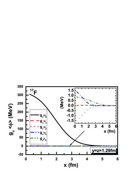
Figure 1: (color online) The distribution of the time-component of the vector potential and the nuclear magnetic potential, i.e., the spatial components of the vector potential, versus $x$ axis for $y=z=1.29$ fm in ¹⁷F.

There is no time-odd magnetic potential in the ground-state of even-even nucleus because of the time-reversal symmetry. For odd-odd or odd A nucleus, the unpaired valence nucleon will give non-vanishing contribution to the nuclear current which provides the time-odd magnetic potentials. The time-component of the vector potential and the nuclear magnetic potential ( the spatial components of the vector potential) in ¹⁷F are given in Fig.1 as functions of $x$ for $y$=$z$=$1.29$ fm. Each component of the nuclear magnetic potential has a peak value around $1.0\sim 1.5$ MeV. Compared with the time-component of the vector potential $V_{0}$, the nuclear magnetic potential is two order smaller in magnitude. However, as the nucleon moves in a potential $\simeq-50$ MeV given by the cancelation of the attractive scalar potential $S(\simeq-400$ MeV) and the repulsive time-component of the vector potential $V_{0}(\simeq+350$ MeV), the magnetic potential will play important role in single-particle properties as will be shown later. Furthermore, Fig.1 shows that the magnetic potential is comparable in magnitude with the iso-vector vector potential provided by the time-component of $\rho$ meson field.

With the presence of the spatial-component of vector field, the magnetic field ${\mathbf{B}}_{n}$ can be defined as ${\mathbf{B}}_{n}=\nabla\times\mbox{\boldmath$\omega$}$. The distribution of nuclear magnetic field ${\mathbf{B}}_{n}$ versus $x$ for $y$=$z$=$1.29$ fm in ¹⁷F are shown in Fig.2. It is found that ${\mathbf{B}}_{n}$ changes rapidly with $x$ and its $x$-component is larger than the other two components. The value used in the estimation of the energy splitting between time reversal conjugate states is around one third of the peak value for the $x$-component of ${\mathbf{B}}_{n}$ for $y$=$z$=$1.29$ fm in ¹⁷F.

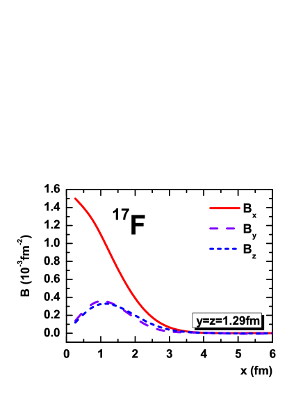
Figure 2: (color online) The nuclear magnetic field ${\mathbf{B}}_{n}(=\nabla\times\mbox{\boldmath$\omega$})$ versus $x$ axis for $y$=$z$=$1.29$ fm in ¹⁷F.

Taking into account the time-odd potentials self-consistently will lead to differences around $3$ MeV for $E_{\sigma}$ and $E_{\omega}$ in Eq.(29). Moreover, the nuclear magnetic potential will lower the potential $(V_{0}+S)({\mathbf{r}})$ in ¹⁷F as shown in Fig.3. However, these differences will cancel with each other. Therefore the time-odd magnetic potentials have small influence on the binding energy, $rms$ radii and quadrupole moment $Q_{0}$ for ¹⁷F. The binding energy per nucleon, $rms$ radii and quadrupole moment for ¹⁷F in triaxial RMF theory with (without) the time-odd magnetic potentials are respectively $7.600(7.589)$ MeV, $2.63(2.63)$ fm and $9.78(9.86)$ fm². The deformation parameters $\beta$ and $\gamma$ for ¹⁷F are respectively 0.08 and 57.14^o after taking into account the time-odd magnetic potentials self-consistently. The $\beta$ value is similar as the previous axial deformed RMF calculation, i.e., $-0.086$Rutz98 .

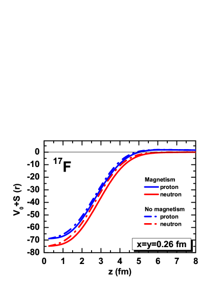
Figure 3: (color online) The potential $(V_{0}+S)({\mathbf{r}})$ for proton and neutron in ¹⁷F with (solid line) or without (dot-dashed line) the time-odd magnetic potentials self-consistently in triaxial RMF theory.

IV.2 Splitting of the time-reversal conjugate single-particle states

The violation of the time reversal invariance will result in the core polarization and lead to the splitting of the the time-reversal conjugate states. Moreover, Because of deformation, the single-particle angular momenta are no longer good quantum numbers. The energies and expectation values of the angular momentum for single-particle time reversal conjugate states $\psi_{\underline{j}}$ and $\psi_{\overline{j}}$ in ¹⁷F are respectively given in Table 1. The expectation values of the orbital angular momentum for the large ($\langle L\rangle$) and small component ($\langle L^{\prime}\rangle$) of the single-particle state are close to their spherical values due to the small $\beta$. As $\gamma$ is close to 60^o, $L_{x}+S_{x}$ is an approximate good quantum number and close to its axial deformed value, from which we can determine the approximate quantum number $ljm$ for the single-particle states as given in Table 1 in this case. One also has $\langle L^{\prime}\rangle\simeq\langle L\rangle\pm 1$ for the state $J=L\pm\frac{1}{2}$. As expected from the estimation in Sec.II, the energy splitting for single-particle time reversal conjugate states in ¹⁷F range from $0.04$ to $0.7$ MeV and larger splitting occurs for states with larger expectation value $\langle L_{x}+S_{x}\rangle$.

Table 1: The energies and expectation values of the angular momentum for single-particle time reversal conjugate states $\psi_{\underline{j}}$ and $\psi_{\overline{j}}$ in ¹⁷F, where $L$ and $L^{\prime}$ are the orbital angular momenta of large and small components respectively, $L_{x}$ and $S_{x}$ are the $x$-component of the orbital angular momenta and spin, and $\Delta\varepsilon=\varepsilon_{\underline{j}}-\varepsilon_{\overline{j}}$.

proton
$l_{j|m|}$	$\psi_{\underline{j}}$					$\psi_{\overline{j}}$
	$\varepsilon$ (MeV)	$L$ $(\hbar)$	$L^{\prime}$ $(\hbar)$	$L_{x}$ $(\hbar)$	$S_{x}$ $(\hbar)$	$\varepsilon$ (MeV)	$L$ $(\hbar)$	$L^{\prime}$ $(\hbar)$	$L_{x}$ $(\hbar)$	$S_{x}$ $(\hbar)$	$\Delta\varepsilon$ (MeV)
$s_{\frac{1}{2}\frac{1}{2}}$	-37.55	0.01	1.01	0.00	-0.50	-37.92	0.01	1.01	0.00	0.50	0.37
$p_{\frac{3}{2}\frac{3}{2}}$	-17.93	1.01	1.93	-1.00	-0.50	-18.60	1.01	1.92	1.00	0.50	0.67
$p_{\frac{3}{2}\frac{1}{2}}$	-17.92	1.01	1.97	-0.41	-0.10	-17.88	1.01	1.97	0.40	0.10	-0.04
$p_{\frac{1}{2}\frac{1}{2}}$	-11.60	1.03	0.28	-0.59	0.10	-11.83	1.03	0.28	0.60	-0.10	0.23
$d_{\frac{5}{2}\frac{5}{2}}$	-1.14	1.98	2.85	-1.98	-0.50	-1.83	1.92	2.83	2.00	0.50	0.69
$d_{\frac{5}{2}\frac{3}{2}}$	-1.10	2.02	2.91	-0.95	-0.20	-1.27	2.03	2.94	1.22	0.25	0.17
$d_{\frac{5}{2}\frac{1}{2}}$	-1.01	2.01	2.93	-0.39	-0.10	-1.08	2.02	2.98	0.12	0.03	0.07
neutron
$l_{j|m|}$	$\psi_{\underline{j}}$					$\psi_{\overline{j}}$
	$\varepsilon$ (MeV)	$L$ $(\hbar)$	$L^{\prime}$ $(\hbar)$	$L_{x}$ $(\hbar)$	$S_{x}$ $(\hbar)$	$\varepsilon$ (MeV)	$L$ $(\hbar)$	$L^{\prime}$ $(\hbar)$	$L_{x}$ $(\hbar)$	$S_{x}$ $(\hbar)$	$\Delta\varepsilon$ (MeV)
$s_{\frac{1}{2}\frac{1}{2}}$	-43.72	0.01	1.01	0.00	-0.50	-44.10	0.01	1.01	0.00	0.50	0.38
$p_{\frac{3}{2}\frac{3}{2}}$	-24.26	1.01	1.93	-1.00	-0.50	-24.96	1.01	1.93	1.00	0.50	0.70
$p_{\frac{3}{2}\frac{1}{2}}$	-23.73	1.01	1.95	-0.48	-0.02	-23.69	1.01	1.96	0.47	0.03	-0.04
$p_{\frac{1}{2}\frac{1}{2}}$	-17.40	1.02	0.33	-0.52	0.02	-17.65	1.02	0.33	0.53	-0.03	0.25
$d_{\frac{5}{2}\frac{5}{2}}$	-6.93	1.93	2.81	-2.00	-0.50	-7.69	1.93	2.82	2.00	0.50	0.76
$d_{\frac{5}{2}\frac{3}{2}}$	-6.35	2.00	2.91	-1.23	-0.21	-6.54	2.00	2.93	1.27	0.22	0.19
$d_{\frac{5}{2}\frac{1}{2}}$	-6.15	1.97	2.90	-0.38	-0.11	-6.22	1.98	2.91	0.34	0.10	0.07

In order to investigate the difference between the energy splitting due to the violation of time reversal invariance from valence neutron and proton, the proton and neutron single-particle levels for time reversal conjugate states in ¹⁷O and ¹⁷F are shown in Fig.4. As a reference, those in ¹⁶O as well as in ¹⁷O and ¹⁷F with time-even potentials only are also given since ¹⁷O or ¹⁷F is nothing but one neutron or proton on top of the ¹⁶O core.

There are the following features: 1) The valence proton (neutron) in ¹⁷F (¹⁷O) will lower the neutron (proton) single particle levels more noticeably than the corresponding proton (neutron) single particle levels; 2) The energy splitting due to the violation of time reversal invariance from valence proton (neutron) in ¹⁷F (¹⁷O) is distinguishable in Fig.4 which denotes the necessity to take into account the time-odd magnetic potentials. In Ref. Rutz98 , the influence of the time-odd magnetic potentials on single-particle energies and the related quantities such as single-particle separate energy has been investigated.

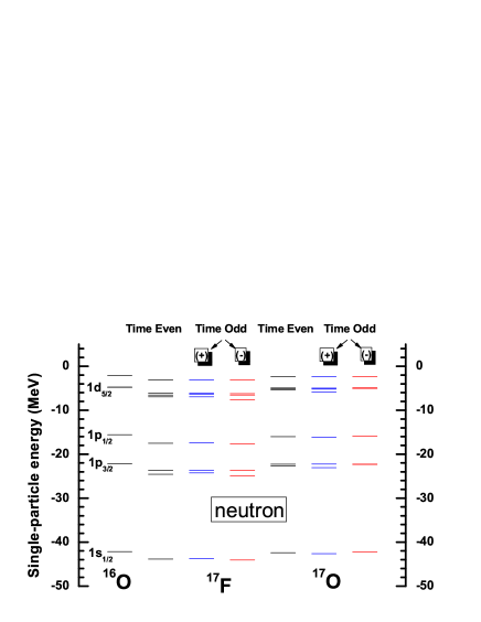
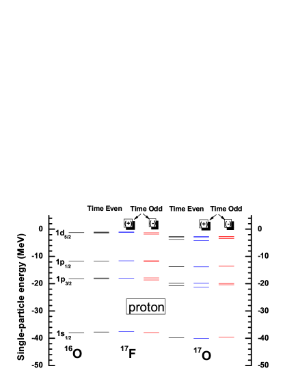
Figure 4: (color online) The proton and neutron single-particle levels for time reversal conjugate states in ¹⁷O and ¹⁷F. Those in ¹⁶O as well as in ¹⁷O and ¹⁷F without time-odd potentials are also given as a reference. The levels with negative angular momentum projection are given in blue (the 3rd and 6th columns) and the levels with positive angular momentum projection are given in red (the 4th and 7th columns) .

The density distribution of the unpaired valence nucleon for ¹⁷O and ¹⁷F as well as the proton, neutron and matter for ¹⁶O, ¹⁷O, and ¹⁷F in $yz$, $zx$, and $xy$ plane are plotted in Figs.5 and 6 respectively, in which the other axis $x$, $y$, and $z$ is integrated respectively. It is interesting to observe that although there are noticeable differences in the energy of the unpaired valence nucleon, the density distributions of the valence proton in ¹⁷F and neutron in ¹⁷O are quite similar to each other and they are corresponding to $1d_{5/2}$ orbits. In Fig.6, the density distributions for proton, neutron and matter in ¹⁷O and ¹⁷F as well as ¹⁶O are shown.

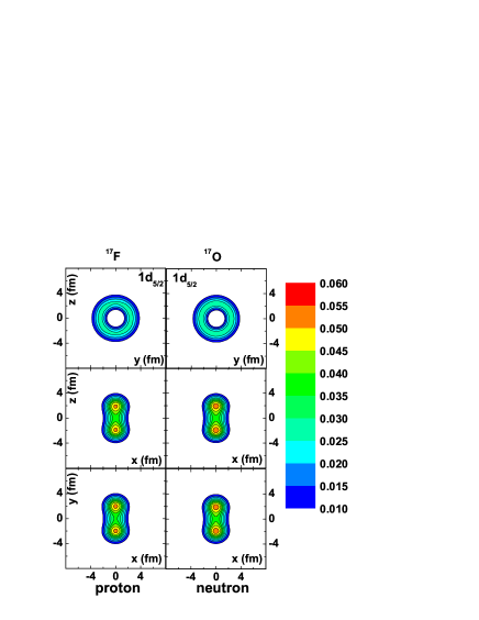
Figure 5: (color online)The density distribution of the unpaired valence nucleon in $yz$, $zx$, and $xy$ plane for ¹⁷F and ¹⁷O while the other axis $x$, $y$, and $z$ is integrated respectively.

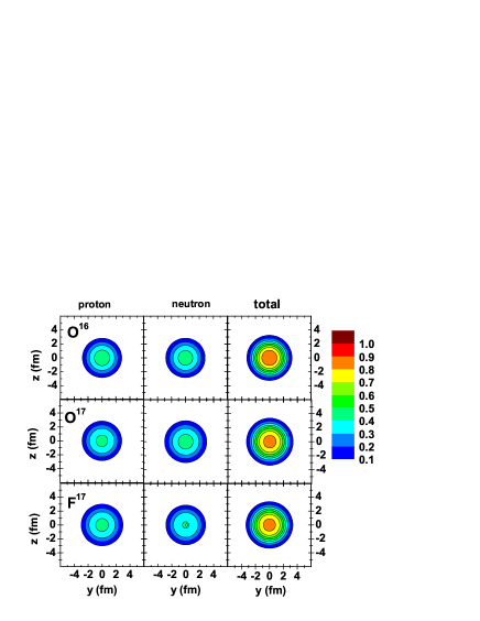
Figure 6: (color online) The proton, neutron and matter density distribution in $yz$, $zx$, and $xy$ plane for ¹⁶O, ¹⁷O, and ¹⁷F, while the other axis $x$, $y$, and $z$ is integrated respectively.

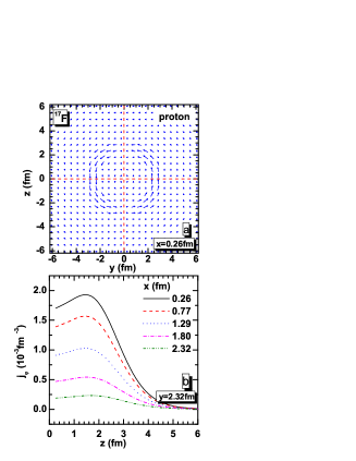
Figure 7: (color online) Upper: The Dirac current for proton in $yz$ plane at x=0.26 fm in ¹⁷F. The direction and length of the arrows respectively represent the orientation and magnitude of current. Lower: The azimuthal component of Dirac current for proton as a function of $z$ with y=2.32 fm and x=0.26, 0.77, 1.29, 1.80, 2.32 fm respectively in ¹⁷F.

IV.3 Current and nuclear magnetic moments

Nuclear magnetic moment is related to the effective electromagnetic current operator Furnstahl89 ; Serot81

$$\hat{J}^{\mu}(x)=Q\bar{\psi}(x)\gamma^{\mu}\psi(x)+\frac{\kappa}{2M}\partial_{\nu}[\bar{\psi}(x)\sigma^{\mu\nu}\psi(x)],$$ (78)

where the field operators are in the Heisenberg representation with $Q\equiv\frac{1}{2}(1-\tau_{3})$, $M$ the nucleon mass, $\sigma^{\mu\nu}=\frac{i}{2}[\gamma^{\mu},\gamma^{\nu}]$, and $\kappa$ the free anomalous gyromagnetic ratio of the nucleon: $\kappa^{p}=1.793$ and $\kappa^{n}=-1.913$. The spatial-component of the current operator is given by,

$${\mathbf{j}}({\mathbf{r}})=Q\psi^{\dagger}({\mathbf{r}})\mbox{\boldmath$\alpha$}\psi({\mathbf{r}})+\frac{\kappa}{2M}\nabla\times[\psi^{\dagger}({\mathbf{r}})\beta\mbox{\boldmath$\Sigma$}\psi({\mathbf{r}})],$$ (79)

where the first term gives the Dirac current ${\mathbf{j}}_{D}({\mathbf{r}})=\psi^{\dagger}({\mathbf{r}})\mbox{\boldmath$\alpha$}\psi({\mathbf{r}})$, which can be decomposed into a orbital (convection) current and a spin current according to Gordon identity, and the second term in Eq. (79) is the so-called anomalous current.

The proton Dirac current in $yz$ plane at x=0.26 fm in ¹⁷F is given in the upper panel in Fig.7 in which the direction and length of the arrows respectively represent the orientation and magnitude of current. It is clearly seen that the Dirac current peaks at the nuclear surface. In order to investigate how the Dirac current change with $x$, the azimuthal component of Dirac current for proton is given for $x=0.26,0.77,1.29,1.80,2.32$ fm respectively as a function of $z$ with $y=2.32$ fm in ¹⁷F. It is found that the Dirac current decreases with $x$. Compared with the density distribution for the valence nucleon in Fig. 5, it is obvious that the current is mainly from the valence nucleon and moves around the nuclear surface in $yz$ plane. In order to see the core polarization effect, the nuclear magnetic moment in the following is more suitable than the current.

In the mean field approximation, the nuclear magnetic moment can be calculated from the expectation value of the current operator in Eq. (79) in ground state,

$$\mu = 2M\int d^{3}r\frac{1}{2}[{\mathbf{r}}\times\langle g.s.|{\mathbf{j}}({\mathbf{r}})|g.s.\rangle]$$

$$= \sum\limits_{i=1}^{A}\int d^{3}r\left[\frac{Mc^{2}}{\hbar c}Q\psi^{\dagger}_{i}({\mathbf{r}}){\mathbf{r}}\times\mbox{\boldmath$\alpha$}\psi_{i}({\mathbf{r}})+\kappa\psi^{\dagger}_{i}({\mathbf{r}})\beta\mbox{\boldmath$\Sigma$}\psi_{i}({\mathbf{r}})\right].$$

Here, $\hbar$ and $c$ are added in order to give the magnetic moment in units of nuclear magneton. The magnetic moment can be divided as the Dirac magnetic moment,

$$\mbox{\boldmath$\mu$}_{D}=\sum\limits_{i=1}^{A}\frac{Mc^{2}}{\hbar c}\int d^{3}rQ\psi^{\dagger}_{i}({\mathbf{r}}){\mathbf{r}}\times\mbox{\boldmath$\alpha$}\psi_{i}({\mathbf{r}}),$$ (81)

and the anomalous magnetic moment,

$$\mbox{\boldmath$\mu$}_{A}=\kappa\int d^{3}r\mu_{A}({\mathbf{r}})=\sum\limits_{i=1}^{A}\kappa\int d^{3}r\psi^{\dagger}_{i}({\mathbf{r}})\beta\mbox{\boldmath$\Sigma$}\psi_{i}({\mathbf{r}}).$$ (82)

The anomalous magnetic moment (proton) density $\mu_{A}({\mathbf{r}})$ distribution in x=0.26 fm plane and the distribution of $\mu_{A}({\mathbf{r}})$ (proton) along $z$ in y=0.26 fm plane, with x=0.26, 0.77, 1.29, 1.80, 2.32 fm respectively in ¹⁷F are plotted in Fig.8. It is found that the anomalous magnetic moment density distribution has the similar character to the Dirac current since they are both mainly dependent on the density distribution of the unpaired valence proton given by Fig.5.

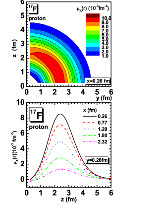
Figure 8: (color online) Upper: The anomalous magnetic moment density $\mu_{A}({\mathbf{r}})$ for proton in $yz$ plane at x=0.26 fm in ¹⁷F. Lower: The anomalous magnetic moment density $\mu_{A}({\mathbf{r}})$ for proton as a function of $z$ with y=0.26 fm and x=0.26, 0.77, 1.29, 1.80, 2.32 fm respectively in ¹⁷F.

Table 2: The magnetic moments of light nuclei near double-closed shells in units of nuclear magneton $\mu_{N}$. The spherical and axial deformed calculations with NL1 are taken from Ref.Hofmann88 .

$\mu$	15O	17O	39Ca	41Ca	15N	17F	39K	41Sc
Exp.	0.72	-1.89	1.02	-1.60	-0.28	4.72	0.39	5.43
Tri.RMF	0.57	-2.00	0.98	-2.13	-0.19	4.893	0.37	6.04
Axi.RMF	0.65	-2.03	0.96	-2.13	-0.29	4.99	0.33	6.07
Sph.RMF	0.66	-1.91	1.17	-1.91	-0.03	5.05	0.72	6.32
Schmidt	0.64	-1.91	1.15	-1.91	-0.26	4.79	0.12	5.79

The magnetic moments in Eq.(IV.3) as well as the Dirac and anomalous magnetic moments in Eqs. (81) and (82) for light nuclei near double-closed shells with A=15, 17, 39, 41 are respectively given in Tables 2 and 3.

Table 3: The Dirac and anomalous magnetic moments ( $\mu_{D}$ and $\mu_{A}$ ) of light nuclei near closed shells in units of $\mu_{\rm N}$. The spherical and axial deformed calculations with NL1 are taken from Ref.Hofmann88 .

$\mu_{D}$	15O	17O	39Ca	41Ca	15N	17F	39K	41Sc
Tri.RMF	-0.11	-0.13	-0.16	-0.28	0.46	3.15	-0.64	4.31
Axi.RMF	-0.13	-0.13	-0.30	-0.22	0.44	3.21	1.50	4.29
Sph.RMF	-	-	-	-	0.59	3.26	1.81	4.54
Schmidt	-	-	-	-	0.33	3.00	1.20	4.00
$\mu_{A}$	15O	17O	39Ca	41Ca	15N	17F	39K	41Sc
Tri.RMF	0.68	-1.87	1.13	-1.85	-0.64	1.75	1.00	1.74
Axi.RMF	0.78	-1.90	1.26	-1.87	-0.73	1.78	-1.17	1.79
Sph.RMF	0.66	-1.91	1.17	-1.91	-0.62	1.79	-1.09	1.79
Schmidt	0.64	-1.91	1.15	-1.91	-0.60	1.79	-1.08	1.79

Table 4: Iso-scalar magnetic moments $\mu(A)=[\mu(Z,N)+\mu(Z+1,N-1)]/2$ of light nuclei near closed shells in units of $\mu_{\rm N}$.

A	Orbit	EXP.	Tri.RMF	Axi.RMFHofmann88	Sph.RMFHofmann88	Schmidt
15	$1p_{1/2}$	0.22	0.19	0.18	0.32	0.19
17	$1d_{5/2}$	1.41	1.45	1.48	1.57	1.44
39	$1d_{3/2}$	0.71	0.67	0.64	0.94	0.64
41	$1f_{7/2}$	1.92	1.96	1.97	2.21	1.94

Table 5: Iso-vector magnetic moments $\mu(A)=[\mu(Z,N)-\mu(Z+1,N-1)]/2$ of light nuclei near closed shells in units of $\mu_{\rm N}$.

A	Exp.	Tri.RMF	Axi.RMFHofmann88	Sph.RMFHofmann88	Schmidt
15	0.501	0.376	0.470	0.345	0.451
17	-3.303	-3.446	-3.510	-3.480	-3.353
39	0.312	0.305	0.315	0.225	0.512
41	-3.513	-4.086	-4.10	-4.115	-3.853

As shown in Table 2, the magnetic moments given by time-odd axial deformed RMF and triaxial deformed RMF calculations reproduce the data well in most cases and are close to each other due to the small $\gamma$ deformation for the nuclei investigated here. The relative large difference for ¹⁵N in Table 2 between the axial and triaxial RMF calculations is mainly from the anomalous part and it is due to the inclusion of $\gamma$ degree of freedom.

The anomalous magnetic moments given by the triaxial RMF calculations are close to those of the spherical ones. While the difference in the total magnetic moment between the spherical and triaxial calculations is mainly from the Dirac magnetic moments due to the core polarization. Without core polarization, the Dirac magnetic moment of neutron particle (hole) should vanish. However, as seen in Table 3, the Dirac magnetic moment for ¹⁵O, ¹⁷O, ³⁹Ca, and ⁴¹Ca contribute around 10% to the total nuclear magnetic moment which is the effect of the core polarization. The core polarization can be taken into account self-consistently in the axial and triaxial calculations but not in the spherical one.

Although the Dirac and anomalous magnetic moments for ³⁹K given by the triaxial RMF calculation have different signs with the other calculations, the triaxial RMF calculation better reproduce the experimental magnetic moment. The triaxial deformed RMF calculation result of ³⁹K gives the deformation parameters $\beta=0.038$ and $\gamma=58.66^{0}$.

The iso-scalar and iso-vector magnetic moments from the spherical, axial and triaxial deformed RMF calculations for light nuclei near the closed shells are given in Tables 4 and 5 in comparison with the data and Schmidt values. As mentioned before, the iso-scalar magnetic moments in deformed RMF calculations are close to the Schmidt values if the core polarization effect has been taken into account self-consistently. The spherical RMF calculations, however, have discrepancies around $10\sim 30\%$ with the data. For the iso-vector magnetic moments, the axial and triaxial deformed RMF calculations agree better with the data than the spherical RMF calculations and the Schmidt values, which demonstrates the importance of the core polarization. In fact, the agreement with the experimental iso-scalar and iso-vector magnetic moments can be improved also in the spherical RMF calculations after considering the core polarization by either the Landau-Migdal approach McNeil86 or the configuration mixing Nedjadi89 .

V Summary

The time-odd triaxial relativistic mean field approach has been developed and applied to the investigation of the ground-state properties of light odd-mass nuclei near double-closed shells. The splitting due to the violation of the time reversal invariance in the single-particle energy has been estimated by reducing the Dirac equation with the time-odd nuclear magnetic potential to Schrodinger equation.

The Dirac equation with time-odd nuclear magnetic potential for nucleon and Klein-Gordon equations for meson fields have been solved self-consistently by expansion on the three dimensional harmonic oscillator basis with PK1. Taking ¹⁷F as an example, the ground-state properties including the binding energy, deformation $\beta$ and $\gamma$, the single-particle energy and the splitting of the time reversal conjugate states, density and current distribution, and magnetic moments, etc., have been examined. It is found that although the non-vanishing spatial-component of the $\omega$ field due to the violation of time reversal symmetry in odd-mass nuclei has small influence on the binding energy, root-mean-square radii and quadrupole moment, it will create a magnetic potential, change the nuclear wave function and result in the core polarization effect which plays important role on the single-particle properties and the magnetic moment. The nuclear magnetic moments for the light double-closed shells nuclei plus or minus one nucleon, including the Dirac, anomalous, iso-scalar, and iso-vector magnetic moments, have been investigated and good agreements with the data have been achieved.

With the time-odd triaxial relativistic mean field approach developed here, it can be expected to describe well not only the light double-closed shells nuclei plus or minus one nucleon, but also the nuclei in the $\gamma$-soft mass region. Investigation along this line is in progress.

Appendix A The basis for solving the Dirac equation

Using the eqs. (50) and (53), the Dirac equation (6) with time-odd magnetic potentials can be written in matrix form,

$$\left(\begin{array}[]{cccc}A_{\alpha^{\prime}\alpha}&{\cal A_{\alpha^{\prime}\overline{\alpha}}}&{\cal B_{\alpha^{\prime}\alpha}}&B_{\alpha^{\prime}\overline{\alpha}}\\ {\cal A_{\overline{\alpha}^{\prime}\alpha}}&A_{\overline{\alpha}^{\prime}\overline{\alpha}}&B_{\overline{\alpha}^{\prime}\alpha}&{\cal B_{\overline{\alpha}^{\prime}\overline{\alpha}}}\\ {-\cal B_{\beta^{\prime}\alpha}}&-B_{\beta^{\prime}\overline{\alpha}}&C_{\beta^{\prime}\alpha}&{\cal C_{\beta^{\prime}\overline{\alpha}}}\\ -B_{\overline{\beta}^{\prime}\alpha}&{-\cal B_{\overline{\beta}^{\prime}\overline{\alpha}}}&{\cal C_{\overline{\beta}^{\prime}\alpha}}&C_{\overline{\beta}^{\prime}\overline{\alpha}}\\ \end{array}\right)\left(\begin{array}[]{c}f_{\alpha}\\ f_{\overline{\alpha}}\\ g_{\alpha}\\ g_{\overline{\alpha}}\end{array}\right)=\varepsilon\left(\begin{array}[]{c}f_{\alpha^{\prime}}\\ f_{\overline{\alpha}^{\prime}}\\ g_{\beta^{\prime}}\\ g_{\overline{\beta}^{\prime}}\end{array}\right).$$ (95)

If the mirror symmetries with respect to three planes ($xy$), ($yz$) and ($xz$) are assumed for all scalar potentials and vector potentials Konig93 , it can be shown that the matrix elements in script letters will vanish. For example, the invariance of the matrix element ${\cal A}_{\alpha^{\prime}\overline{\alpha}}$,

$${\cal A}_{\alpha^{\prime}\overline{\alpha}} = \frac{1+(-1)^{n^{\prime}_{x}+\tilde{n}_{x}+1}}{2}(-1)^{\tilde{n}_{x}+\tilde{n}_{y}+1}\cdot(-1)^{\frac{\tilde{n}_{y}-n^{\prime}_{y}}{2}}$$ (97)

$$\cdot\int d^{3}r\phi_{n^{\prime}_{x}}(x)\phi_{n^{\prime}_{y}}(y)\phi_{n^{\prime}_{z}}(z)(V_{0}+M^{*})\phi_{\tilde{n}_{x}}(x)\phi_{\tilde{n}_{y}}(y)\phi_{\tilde{n}_{z}}(z)$$

under the operation $x\rightarrow-x$ will leads to ${\cal A}_{\alpha^{\prime}\tilde{\alpha}}=0$. After similar operation for $y$ and $z$, the matrix in Eq.(95) can be written as,

$$\left(\begin{array}[]{cccc}A_{\alpha^{\prime}\alpha}&B_{\alpha^{\prime}\overline{\alpha}}&0&0\\ -B_{\overline{\beta}^{\prime}\alpha}&C_{\overline{\beta}^{\prime}\overline{\alpha}}&0&0\\ 0&0&A_{\overline{\alpha}^{\prime}\overline{\alpha}}&B_{\overline{\alpha}^{\prime}\alpha}\\ 0&0&-B_{\beta^{\prime}\overline{\alpha}}&C_{\beta^{\prime}\alpha}\\ \end{array}\right)\left(\begin{array}[]{c}f_{\alpha}\\ g_{\overline{\alpha}}\\ f_{\overline{\alpha}}\\ g_{\alpha}\\ \end{array}\right)=\varepsilon\left(\begin{array}[]{c}f_{\alpha^{\prime}}\\ g_{\overline{\beta}^{\prime}}\\ f_{\overline{\alpha}^{\prime}}\\ g_{\beta^{\prime}}\\ \end{array}\right),$$ (110)

which indicates that the space $\{\psi_{i}\}$ can be reduced into two subspace $\{\psi_{\underline{j}}\}$ and $\{\psi_{\overline{j}}\}$ in Eq.(59).

References

• (1) R. J. Blin-Stoyle, Rev. Mod. Phys. Vol. 28, 75(1956) .
• (2) B. H. Wildenthal and W. Chung, Mesons in Nuclei, Vol. II, edited by M. Rho and D. Wilkinson (North-Holland, Amsterdam, 1979), p. 721.
• (3) A. Arima, Prog. Part. Nucl. Phys. 11, 53(1984).
• (4) N. J. Stone, Table of Nuclear Magnetic Dipole and Electric Quadrupole Moments, NNDC, http://www. BNL. gov,2001 and the references therein.
• (5) H. Ueno et al., Phys. Rev. C53, 2142(1996) and the references therein.
• (6) A. Arima, H. Horie, Prog. Theor. Phys. 11, 509(1954).
• (7) M. Chemtob, Nucl. Phys. A123, 449 (1969).
• (8) A. Arima, K. Shimizu, W. Bentz and H. Hyuga, Adv. Nucl. Phys. 18, 1 (1987).
• (9) U. Hofmann, P. Ring, Phys. Lett. B214, 307(1988).
• (10) S. Ichii, W. Bentz and A. Arima, Nucl. Phys. A464, 575(1987).
• (11) I. S. Towner and F. C. Khanna, Nucl. Phys. A399, 334 (1983).
• (12) B. D. Serot and J. D. Walecka, Adv. Nucl. Phys. Vol. 16, 1(1986).
• (13) P. G. Reinhard, Rep. Prog. Phys. 52, 439(1989).
• (14) P. Ring, Prog. Part. Phys. Vol. 37, 193(1996).
• (15) J. Meng, H. Toki, S. G. Zhou, S. Q. Zhang, W. H. Long, L. S. Geng, Prog. Part. Nucl. Phys. (2006) in press.
• (16) J. Meng, P. Ring, Phys. Rev. Lett. 77, 3963(1996) .
• (17) J. Meng, P. Ring, Phys. Rev. Lett. 80, 460(1998).
• (18) N. K. Glendenning, Campact stars (Springer-Verlag, New York, 1997).
• (19) A. Arima, M. Harvey, and K. Shimizu, Phys. Lett. 30B, 517 (1969).
• (20) K. T. Hecht, A. Adler, Nucl. Phys. A137, 129 (1969).
• (21) J. N. Ginocchio, Phys. Rev. Lett. 78, 436(1997).
• (22) J. Meng, Phys. Rev. C57, 1229(1998).
• (23) J. Meng, K. Sugawara-Tanabe, S. Yamaji and A. Arima, Phys. Rev. C59, 154(1999).
• (24) S. G. Zhou, J. Meng, and P. Ring, Phys. Rev. Lett. 91, 262501(2003).
• (25) L. S. Geng, H. Toki, and J. Meng, Prog. Theor. Phys. 113, 785(2005).
• (26) A. Bouyssy, S. Marcos and J. CF. Mathiot, Nucl. Phys. A415, 497(1984).
• (27) H. Kurasawa and T. Suzuki, Phys. Lett. 165B, 234(1985).
• (28) L. D. Miller, Ann. Phys. 91, 40(1975).
• (29) H. Ohtsubo, M. Sano, and M. Morita, Prog. Theor. Phys. 49, 877 (1973) .
• (30) M. Bawin, C. A. Hughes, and G. L. Strobel, Phys. Rev. C28, 456 (1983) .
• (31) J. R. Shepard, E. Rost, C. -Y. Cheung, and J. A. McNeil, Phys. Rev. C37, 1130(1988).
• (32) J. A. McNeil, R. D. Amado, C. J. Horowitz, M. Oka, J. R. Shepard, and D. A. Sparrow, Phys. Rev. C34, 746(1986).
• (33) R. J. Furnstahl, C. E. Price, Phys. Rev. C40, 1398(1989).
• (34) H. Madokoro, J. Meng, M. Matsuzaki, and S. Yamaji, Phys. Rev. C62, 061301(R) (2000).
• (35) J. König, P. Ring, Phys. Rev. Lett. 71, 3079(1993).
• (36) J. Meng, J. Peng, S. Q. Zhang, and S.-G. Zhou, Phys. Rev. C73, 037303 (2006).
• (37) M. Beender, K. Rutz, P.-G. Reinhard, J. A. Maruhn, Eur. Phys. J. A7, 467 (2000).
• (38) M. Girod, B. Grammaticos, Phys. Rev. C27, 2317 (1983).
• (39) W. Koepf and P. Ring, Nucl. Phys. A493, 61(1989).
• (40) D. Vautherin, Phys. Rev. C7, 296 (1973).
• (41) Wenhui Long, J. Meng, Nguyen Van Giai, and Shan-Gui.Zhou, Phys. Rev. C69, 034319(2004).
• (42) K. Rutz, M. Bender, P.-G. Reinhard, J. A. Maruhn, Nucl. Phys. A634, 67 (1998).
• (43) B. D. Serot, Phys. Lett. 107B, 263 (1981).
• (44) Y. Nedjadi and J. R. Rook, J. Phys. G: Nucl. Part. Phys. 15, 589(1989).