[

A new variable in flow analysis

Abstract

We have used a simple spectrum distribution which was derived from a hydrodynamical equation[12] to fit the data of the STAR group. It is found that it can fit the $v_{2}$ of STAR group very well. We have found that $v_{2}$ is sensitive to both the effective temperature of particles and the expanding velocity. We have suggested a new variable ${\bf z}$ to be used in the flow analysis. This new variable will measure the correlation of particles momentum components. We have also shown that one of the $x$ or $y$ direction in the reaction plane is the direction which has the largest variance.

]

Recently, the study of elliptic flow has attracted attention of both theoreticians and experimentalists.[1, 2, 3, 4, 5, 6, 7, 8]. It was argued that an anisotropic distribution of final state particles with respect to the reaction plane can be used to reflect the strong re-interaction among quarks and gluons in the initial state.

The calculation of $v_{2}$, the anisotropic distribution of final state particles is always done in the following two ways:(1): we determine the reaction plane first, then we calculate the average of $\langle\cos(2(\phi-\phi_{R}))\rangle$. Here $\phi_{R}$ is the azimuthal angle of the reaction plane and $\phi$ is the azimuthal angle of particles in the Lab frame. (2): using the pairwise azimuthal correlations[11] to calculate the $v_{2}$. The second method has an advantage over the first method that no reaction plane is needed to be determined. But a prior knowledge on the distribution of $P(\phi)$ is needed to be known for the second method. The biggest problem for the first method is to determine the reaction plane. There are several methods are used in data analysis. In RHIC, the so called second harmonic event plane is widely used in the data analyzes.

However, it seems to the authors that we still not clear what we really have measured in the experiment. To discuss this question, we will use the spectrum distribution in Ref.[12]. This spectrum distribution is a solution for a hydrodynamical equation and it can be expressed as

$$P({\bf p})\propto\exp(-\frac{(p_{x}-mv_{x})^{2}}{2mT_{x}}-\frac{(p_{y}-mv_{y})^{2}}{2mT_{y}}).$$ (1)

Here ${\bf v}=(v_{x},v_{y})$ is the expanding velocity of particles. $T_{x}$ and $T_{y}$ are effective temperatures of $x$ component and $y$ component of particles momentum[12]. The above picture can be understood in the following way: AA collision will form a QGP or a dense hadron phase at the initial state. Due to the initial asymmetry collisions, it is expected that the effective temperature will be different in $x$ and $y$ components. After some time, the hadron gas are formed. This hadron gas will expand in velocity ${\bf v}$. This distribution is relative to the reaction plane.

Using this equation, we will calculate $v_{2}$ using following three variables. They are ${\bf p}$, ${\bf\tilde{p}}={\bf p}-{\bf\bar{p}}$, and ${\bf z}=(\frac{\tilde{p}_{x}}{\langle(\tilde{p}_{x})^{2}\rangle},\frac{\tilde{p}_{y}}{\langle(\tilde{p}_{y})^{2}\rangle})$. Here $\langle\tilde{p}_{x}^{2}\rangle$ and $\langle\tilde{p}_{y}^{2}\rangle$ are second moments in $x$ and $y$ direction respectively which are defined as

$$\langle\tilde{p}_{x}^{2}\rangle = \int P({\bf\tilde{p}})\tilde{p}_{x}^{2}d{\bf\tilde{p}}$$ (2)

$$\langle\tilde{p}_{y}^{2}\rangle = \int P({\bf\tilde{p}})\tilde{p}_{y}^{2}d{\bf\tilde{p}}.$$ (3)

Then we will calculate $v_{2}$ using the following formula:

$$v_{2}=\frac{\int P({\bf u})\frac{u_{x}^{2}-u_{y}^{2}}{u_{x}^{2}+u_{y}^{2}}d{\bf u}}{\int P({\bf u})d{\bf u}}$$ (4)

Here ${\bf u}$ is one of the three variables in the above formula. It is easily checked that

$$v_{2}(z)=0$$ (5)

for all cases.

$$v_{2}(\tilde{p})=0$$ (6)

when $T_{x}=T_{y}$; but $v_{2}(\tilde{p})$ is not zero when $T_{x}\neq T_{y}$. $v_{2}({\bf p})$ is not zero and its value is shown in Fig.1. It is interesting to notice that flow may be caused by the expansion velocity $v$ and the ”effective temperature” if we use variables ${\bf p}$ and ${\bf\tilde{p}}$. However, there is no flow to be observed if we use variable $z$.

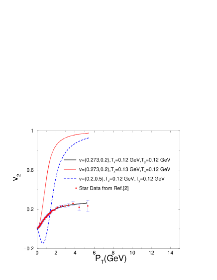
FIG. 1.: $v_{2}$ vs. $p_{t}$.

From Fig.1, we notice that:(1) the differences between $T_{x}$ and $T_{y}$ can cause strong flow. (2): The difference between $v_{x}$ and $v_{y}$ also cause flow. It seems that the data does not support the assumption that $T_{x}$ is different from $T_{y}$. But we need to point out that this results is model dependent. One interesting thing is that this model can fit the data very well especially in the larger $p_{T}$ region.

For elliptic flow analysis, we are more interested in the distribution of particles in momentum space or azimuthal angle space. We would like to see the relative differences between $x$-components and $y$-components of particles momentum. The difference between $T_{x}$ and $T_{y}$ might be caused by the initial flow in QGP phase. But $T_{x}$ and $T_{y}$ are measurements which could tell us the absolutely value of particles momentum in different direction. Besides this effective temperatures difference we also like to find a correlation inside the distribution of $P({\bf p_{x},p_{y}})$. From the above simple model, we find that $z$ variable is a proper variable for this purpose. We would like it can be used in the data analysis.

To understand the meaning of the flow, we will start from the transverse momentum sphericity tensor defined by

$$S_{ij}=\sum_{\nu=1}^{M}u_{i}(\nu)u_{j}(\nu),$$ (7)

where $u_{i}(i=1,2)$ is the $i$-th component of the variable $u$. As above, this ${\bf u}$ can be one of three variables mention above. To be more clearly, we have the following matrix.

$\displaystyle\left[\begin{array}[]{cc}\sum_{\nu=1}^{M}u_{1}^{2}(\nu)&\sum_{\nu=1}^{M}u_{1}(\nu)u_{2}(\nu)\\ \sum_{\nu=1}^{M}u_{1}(\nu)u_{2}(\nu)&\sum_{\nu=1}^{M}u_{2}^{2}(\nu)\end{array}\right]$

It is clear that the eigenvalue of this matrix are

$$\lambda_{1} = \frac{S_{11}+S_{22}+\sqrt{(S_{11}-S_{22})^{2}+4S_{12}^{2}}}{2},$$ (8)

$$\lambda_{2} = \frac{S_{11}+S_{22}-\sqrt{(S_{11}-S_{22})^{2}+4S_{12}^{2}}}{2}.$$ (9)

Its eigenvectors determine the $x$ direction and $y$ direction of the reaction plane if we take ${\bf u}={\tilde{p}}$. However transverse momentum method is widely used in the data analysis to determine the direction of reaction plane. The reaction plane is determined by using the following formula:

$${\bf Q}=\sum_{i=1}^{M}\omega_{i}{\bf u}.$$ (10)

Here $\omega_{i}=1$ when particles rapidity is big than zero and $\omega_{i}=-1$ when particles rapidity is less than zero. The basic idea behind this method is that the total transverse momentum of the system in the $y$ direction of the reaction plane is zero and the symmetry of the collision system in the direction of $\theta$ to $\theta+\pi$. Here $\theta$ is the polar angle. Can this two methods give the same reaction plane?

We will give a positive answer to this question under the condition that the multiplicity of event is infinity in this paragraph. When we determine the two eigenvectors, then $S_{12}=0$ in this new frames. If we use Eq.(10) to determine the reaction plane first, then we can also find that $S_{12}$ will be zero in the frame due to the symmetry of $u_{2}\leftrightarrow-u_{2}$. We will show that there is only one vector in the $x-y$ planes which lead the value of $S_{12}$ is zero. Suppose that a new axis which has angle relative to the reaction plane is $\theta$. It is easily checked that the new quantity in this new frame is

$$u_{x}^{\prime}(\nu) = u_{x}^{R}(\nu)\cos(\theta)+u_{y}^{R}(\nu)\sin(\theta)$$ (11)

$$u_{y}^{\prime}(\nu) = -u_{x}^{R}(\nu)\sin(\theta)+u_{y}^{R}(\nu)\cos(\theta)$$ (12)

Here the superscript $R$ refers that those quantities are in the reaction plane frame. ${\bf u^{\prime}(\nu)}$ is the variable in the new frame. Then

$$S_{12}^{\prime}=\sum_{\nu=1}^{M}u_{x}^{\prime}(\nu)u_{y}^{\prime}(\nu)=\frac{[S_{22}^{R}-S_{11}^{R}]\sin(2\theta)}{2}.$$ (13)

It is clear that $S_{12}^{\prime}$ is zero only when $\theta=0$ or $\pi$ or $S_{11}^{R}=S_{22}^{R}$. For the first case, it means that $S_{12}^{\prime}=0$ when it is in the reaction plane frame. When $S_{11}^{R}=S_{22}^{R}$, the shape of $u^{T}Su$ is circle in momentum space. The eigenvector for this matrix is arbitrary. Therefore, we have shown that the transverse momentum method and sphericity tensor give the same reaction plane when the multiplicity is huge.

Then $\alpha$ which is used to measure the asymmetry distribution of particles in the momentum can be calculated in the following ways.

$$\alpha=\frac{\lambda_{1}-\lambda_{2}}{\lambda_{1}+\lambda_{2}}=\frac{(\sum_{\nu=1}^{M}u_{x}^{R}(\nu))^{2}-(\sum_{\nu=1}^{M}u_{y}^{R})^{2}}{(\sum_{\nu=1}^{M}u_{x}^{R}(\nu))^{2}+(\sum_{\nu=1}^{M}u_{y}^{R}(\nu))^{2}}$$ (14)

Using Eq(9), we have

$$\alpha=\frac{\sqrt{(S_{11}-S_{22})^{2}+4S_{12}^{2}}}{S_{11}+S_{22}}.$$ (15)

Taking ${\bf u=p_{t}}$, $\alpha$ can be expressed as

$$\alpha=\frac{1}{M}\sum_{\nu=1}^{M}\cos(2\phi_{\nu}^{R})\frac{p_{t}(\nu)^{2}}{\langle p_{t}^{2}\rangle}$$ (16)

Here $\langle p_{t}^{2}\rangle=\frac{1}{M}\sum_{\nu=1}^{M}{\bf p_{t}^{2}}$ are the transverse momentum square average for the event. $M$ is the multiplicity for the event. Then we have

$$\langle\alpha\rangle=\langle\cos(2\phi_{\nu}^{R})\frac{p_{t}(\nu)^{2}}{\langle p_{t}^{2}\rangle}\rangle.$$ (17)

This average is taken over all events. If the transverse momentum is fixed, then we have

$$\alpha(p_{t})=v_{2}(p_{t}).$$ (18)

Therefore, we can calculate $v_{2}(p_{t})$ using Eq.(15) directly. If we choose ${\bf u}={\bf z}=(z_{1},z_{2})=(\frac{\tilde{p_{x}}}{\sum\tilde{p_{x}}^{2}},\frac{\tilde{p_{y}}}{\sum\tilde{p_{y}}^{2}})$, then we find that the matrix for $z$ becomes to

$\displaystyle\left[\begin{array}[]{cc}1&\sum_{\nu=1}^{M}z_{1}(\nu)z_{2}(\nu)\\ \sum_{\nu=1}^{M}z_{1}(\nu)z_{2}(\nu)&1\end{array}\right]$

Then the $\alpha$ for this new variable will be

$$\alpha({\bf z})=|S_{12}(z)|=\frac{|S_{12}|}{\sqrt{S_{11}S_{22}}}.$$ (19)

When particles rapidity window is huge and number of particle is infinity for each event, we can write

$$S_{11} = \int P({\bf\tilde{p}}){\tilde{p}_{x}}{\tilde{p}_{x}}d{\tilde{p}_{x}}d{\tilde{p}_{y}}$$ (20)

$$S_{22} = \int P({\bf\tilde{p}}){\tilde{p}_{y}}{\tilde{p}_{y}}d{\tilde{p}_{x}}d{\tilde{p}_{y}}$$ (21)

$$S_{12} = \int P({\bf\tilde{p}}){\tilde{p}_{x}}{\tilde{p}_{y}}d{\tilde{p}_{x}}d{\tilde{p}_{y}}$$ (22)

Therefore

$$\alpha(z)=\frac{|\int P({\bf\tilde{p}}){\tilde{p}_{x}}{\tilde{p}_{y}}d{\tilde{p}_{x}}d{\tilde{p}_{y}}|}{\sqrt{\int P({\bf\tilde{p}}){\tilde{p}_{x}}{\tilde{p}_{x}}d{\tilde{p}_{x}}d{\tilde{p}_{y}}\int P({\bf\tilde{p}}){\tilde{p}_{y}}{\tilde{p}_{y}}d{\tilde{p}_{x}}d{\tilde{p}_{y}}}}.$$ (23)

Thus $\alpha(z)$ actually measures the correlation between the two component of particles. If the particles are emitted randomly, $\alpha(z)=0$. On the other hand, if particles are emitted always in the a particular direction, say $p_{x}=p_{y}$, then $\alpha(z)=1$. It is easily checked that

$$\alpha(\tilde{p})=\sqrt{1+4\frac{t}{(1+t)^{2}}(\alpha(z)^{2}-1)}.$$ (24)

Here $t=\frac{S_{11}}{S_{22}}$. It is interesting to notice that when $t=1$, then $\alpha({\tilde{p}})=\alpha(z)$. It is easily seen that $\alpha({\tilde{p}})\geq\alpha(z)$. If $t=0$, then $\alpha({\tilde{p_{t}}})=1$ which corresponds to the case particles are emitted only in the $y$ direction. The advantage of $\alpha(z)$ over $\alpha({\tilde{p_{t}}})$ is clear: it depends on a dimensionless variable; it measures the correlations between the components of particles momentum.

If we take ${\bf u=p_{t}}$ and ${\bf y}=(\frac{p_{x}}{\langle p_{x}^{2}\rangle},\frac{p_{y}}{\langle p_{y}^{2}\rangle})$, then we will have similar expressions as above. The only difference is that we need to use varible ${\bf p_{t}}$ and ${\bf y}$ to take the place of variables ${\tilde{p_{t}}}$ and ${\bf z}$ in above expressions.

If $\alpha(z)$ is very small, we have

$$\alpha(\tilde{p})\sim\frac{|1-t|}{1+t}=\frac{|S_{11}-S_{22}|}{S_{11}+S_{22}}.$$ (25)

Thus $\alpha({\tilde{p}})$ measure the ratio between the difference of the variance in $x$ and $y$ directions and the sum of the variance in $x$ and $y$ directions. The detail information of $\alpha(z)$ will not be observed.

One of interesting things about the matrix of variable $z$ is that its eigenvector is always along the direction $(\frac{1}{\sqrt{2}},\frac{1}{\sqrt{2}})$ or $(\frac{1}{\sqrt{2}},\frac{-1}{\sqrt{2}})$. Due to the fact that the finite multiplicity in the collisions, the ”estimated reaction plane” will fluctuate randomly. Finally, we need to point out that this estimated reaction plane is quite different from the reaction plane estimated using variable ${\bf\tilde{p}}$ since they are in different variable spaces.

In the experiment, experimentalists normally used ${\bf u}=\frac{\bf{p_{t}}}{|{\bf p_{t}}|}=(\cos(\phi),\sin(\phi))$ in the analysis. The matrix for $x$ is

$\displaystyle\left[\begin{array}[]{cc}\sum_{\nu=1}^{M}\cos^{2}(\phi_{\nu})&\sum_{\nu=1}^{M}\cos(\phi_{\nu})\sin(\phi_{\nu})\\ \sum_{\nu=1}^{M}\cos(\phi_{\nu})\sin(\phi_{\nu})&\sum_{\nu=1}^{M}\sin^{2}(\phi_{\nu})\end{array}\right]$

When the system transform to eigenvectors frame, we have

$$\sum_{\nu=1}^{M}\sin(\phi_{\nu}-\phi_{R})\cos(\phi_{n}u-\phi_{R})=\frac{1}{2}\sum_{\nu=1}^{M}\sin 2(\phi_{\nu}-\phi_{R})=0.$$ (26)

This is the way to calculate the reaction plane azimuthal angle ($\phi_{R}$) in RHIC data analyses.

We can construct other varibles to dertermine the high-order harmonics reaction plane. For example, when $n=4$, we can take ${\bf u}=(\frac{2p_{x}p_{y}}{|{\bf p_{t}}|^{2}},\frac{p_{x}^{2}-p_{y}^{2}}{|{\bf p_{t}}|^{2}})=(\sin(2\phi),\cos(2\phi))$. If we calculate the matrix in the corresponding eigenvector frame, we have

$$\sum_{\nu=1}^{M}\sin 2(\phi_{\nu}-\phi_{R})\cos(2(\phi_{\nu}-\phi_{R}))$$ (27)

$$= \frac{1}{2}\sum_{\nu=1}^{M}\sin 4(\phi_{\nu}-\phi_{R})=0.$$ (28)

This is the way to calculate the fourth harmonic reaction plane as metioned in the Ref.[9]. In general this estimated reaction plane should be different from the estimated second harmonic reaction plane since they are estimated for different variables. The corresponding $\alpha$ for this matrix is $v_{4}$.

We have shown in the above that when the multiplicity is huge, transverse momentum and spherecity matrix will give the same ”estimated” reaction plane for variable ${\bf u}$ as long as they have symmetry $u_{y}\leftrightarrow-u_{y}$. However, we know that this estimated reaction plane is quite different for different variable ${\bf u}$. What is the physical meaning of the direction estimated by sphericity matrix and transverse momentum? We will show in the next paragraph that this eigenvectors directions actually gives the direction where the variance is the maximum.

Suppose that ${\bf u}$ is a vector ($2\times 1$ matrix) in the lab frame and we will try to find a new frame such that the new variable ${\bf u^{\prime}}$ has the largest variance along a axis in the frame. Suppose $a^{T}$ is a $2\times 2$ matrix, then the new variable $u^{\prime}$will be

$$u_{i}^{\prime}={\bf a_{i}^{T}}{\bf u},~{}~{}~{}~{}~{}~{}~{}i=1,2.$$ (29)

Here ${\bf a_{i}^{T}}=(a_{i1},a_{i2})$. Then its variance is

$$\sum_{\nu=1}^{M}(u_{i}^{\prime}(\nu))u_{i}^{\prime T}(\nu)={\bf a_{i}^{T}uu^{T}a_{i}}={\bf a_{i}^{T}}S{\bf a_{i}},~{}~{}~{}~{}~{}~{}~{}i=1,2.$$ (30)

if we take a constraint that ${\bf a_{i}^{T}a_{i}}=1$. Then we can construct the following Lagrange multipliers

$$L({\bf a_{i}})={\bf a_{i}^{T}}S{\bf a_{i}}-\lambda({\bf a_{i}^{T}a_{i}}=1).$$ (31)

Taking derivation with ${\bf a_{i}}$, we have

$$\frac{\partial L}{\partial{\bf a_{i}}}=2S{\bf a_{i}}-2\lambda{\bf a_{i}}$$ (32)

Setting this value to zero, we have

$$S{\bf a_{i}}=\lambda{\bf a_{i}},$$ (33)

and

$$\sum_{\nu=1}^{M}(u_{i}^{\prime}(\nu))^{T}u_{i}^{\prime}(\nu)=\lambda_{i};i=1,2$$ (34)

This tell us that when we choose one of the eigenvector as $a_{1}$, then its maximum variate will be the eigenvalue. We will choose the largest eigenvalue. It is also easily to prove that if we choose $a_{2}$ as another eigenvalue. Then the $S_{12}$ will be zero for variable $u^{\prime}$. Therefore we have shown here that the one of the eigenvectors actually gives us the direction where the variance is the largest. For another eigenvector which give us another direction which has a property that $S_{12}$ will be zero (in other words, its component will be uncorrelated with the first component). The largest variance for our case is the largest eigenvalue.

Conclusions: It has been shown that the $v_{2}$ measured in the data reflects the information on the expanding velocity, effective temeparature in $x$ and $y$ components and correlation between different components of the particles momentum. However due to the fact that the correlation between different momentum of particles are small. Therefore we redefine a new variable $z$ which can be used in the data analysis. We belived that $v_{2}(z)$ is small but can show us the information on the correlation between different components of particles. We have also shown that estimated reaction plane will be different if we choose different variables in the data analysis. The two directions in the reaction plane can be undersood as the biggest variance directions of the data. One of the interesting thing is that, the model can fit the data quite well. This model suggests that the effective temparature for different directions of momentums are almost the same.

The authors thank R. C. Hwa, S. Padula for for helpful discussions. This work was supported by the National Natural Science Foundation of China under Contract No.10275015” . QHZ thank C. Gale for his help during the preparation of the paper.

REFERENCES

[1]
S. S. Adler et al., Phys. Rev. Lett. 91 , 182301 (2003).
[2]
J. Adms et. al., Phys. Rev. Lett. 92, 052302 (2004);
J. Adms et. al., Phys. Rev. Lett. 92, 062301 (2004);
C. Adler et. al., Phys. Rev. Lett. 90, 032301 (2003);
C. Adler et. al., Phys. Rev. C 66, 034904 (2002);
C. Adler et. al., Phys. Rev. Lett. 89, 132301 (2002);
C. Adler et. al., Phys. Rev. Lett. 89, 182301 (2001);
C. Adler et. al., Phys. Rev. Lett. 86, 402 (2001).
[3]
B.B. Back et al., nucl-ex/0406021.
B.B. Back et al., Phys. Rev. Lett 89, 222301 (2002).
[4]
J. Barrette et al., Phys. Rev. Lett. 70, 2996 (1993),
Phys. Rev. C 56, 3254 (1997),
Phys. Rev. C 55, 1420 (1997).
[5]
P. Chung et al., Phys. Rev. C 66, 021901 (2002);
[6]
M. Gyulassy and L. McLerran, nucl-th/0405013.
[7]
P. F. Kolb and U. Heinz, nucl-th/0305084;
U. Heinz and S. M. H. Wong,
Phys. Rev. C 66, 014907 (2002).
[8]
J. Y. Ollitrault, Phys. Rev. D 48 ,1132 (1993),
Phys. Rev. D 46, 229 (1992).
[9]
A. M. Poskanzer and S. A. Voloshin, Phys. Rev. C 58, 1671 (1998).
[10]
Z. W. Lin and D. Molnar, Phys. Rev. C68, 044901 (2003);
Z. W. Lin and C. M. Ko, Phys. Rev. Lett. 89, 202302 (2002);
D. Monar and S. Voloshin, Phys. Rev. Lett. 91, 092301 (2003).
[11]
S. Wang et al., Phys. Rev. C 44, 1091 (1991);
R. Lacey et al., Phys. Rev. Lett. 70, 1224 (1993).
[12]
M. Csanad, T. Csorgo and B. Lorstad, nucl-th/0310040;
T. Csorgo, F. Grassi, Y. Hama, T. Kodama, Phys. Lett. B565,107 (2003);
T. Csorgo, S.V. Akkelin, Y. Hama, B. Lukacs and Y. M. Sinyukov,
Phys. Rev. C67, 034904 (2003).