Multiplicity Fluctuations in Hadron-Resonance Gas

Abstract

The charged hadron multiplicity fluctuations are considered in the canonical ensemble. The microscopic correlator method is extended to include three conserved charges: baryon number, electric charge and strangeness. The analytical formulae are presented that allow to include resonance decay contributions to correlations and fluctuations. We make the predictions for the scaled variances of negative, positive and all charged hadrons in the most central Pb+Pb (Au+Au) collisions for different collision energies from SIS and AGS to SPS and RHIC.

I Introduction

The statistical models have been successfully used to describe the data on hadron multiplicities in relativistic nucleus-nucleus (A+A) collisions (see, e.g., Ref. stat-model ; FOC ; FOP and recent review BMST ). The applications of the statistical model to elementary reactions and/or to rare particles production have stimulated an investigation of the relations between different statistical ensembles. In A+A collisions one prefers to use the grand canonical ensemble (GCE) because it is the most convenient one from the technical point of view. The canonical ensemble (CE) ce-a ; ce ; ce-b ; ce-c ; ce-d ; ce-e or even the microcanonical ensemble (MCE) mce have been used in order to describe the $pp$, $p\bar{p}$ and $e^{+}e^{-}$ collisions when a small number of secondary particles is produced. At these conditions the statistical systems are far away from the thermodynamic limit, the statistical ensembles are not equivalent, and the exact charge, or both energy and charge conservation, laws have to be taken into account. The CE suppression effects for particle multiplicities are well known in the statistical approach to hadron production, for example, the suppression in a production of strange hadrons ce-c , antibaryons ce-d , and charmed hadrons ce-e when the total numbers of these particles are small (smaller than or equal to 1). The different statistical ensembles are not equivalent for small systems. When the system volume increases, $V\rightarrow\infty$, the average quantities in the GCE, CE and MCE become equal to each other, i.e., all statistical ensembles are thermodynamically equivalent.

The fluctuations in high energy nuclear collisions (see, e.g., Refs. fluc1 ; fluc2 ; fluc3 ; fluc4 ; fluc5 ; step1 ; Jeon-Koch ; fluc6 ; fluc7 ; fluc7a ; fluc7b ; fluc8 ; MGMG ; KGB and references therein) reveal new physical information and can be closely related to the phase transitions in the QCD matter. The particle number fluctuations for relativistic systems in the CE were calculated for the first time in Ref. ce-fluc for the Boltzmann ideal gas with net charge equal to zero. These results were then extended to quantum statistics and non-zero net charge in the CE ce2-fluc ; ce3-fluc ; bec ; bose-fluc and to the MCE mce-fluc ; mce2-fluc , and compared to the corresponding results in the GCE (see also Refs. turko ; Hauer ). Expressed in terms of the scaled variances, the particle number fluctuations have been found to be suppressed in the CE and MCE comparing to the GCE. This suppression survives in the limit $V\rightarrow\infty$, so the thermodynamical equivalence of all statistical ensembles refers to the average quantities, but is not applied to the scaled variances of particle number fluctuations.

The aim of the present paper is to extend a microscopic correlator method to treat the hadron-resonance gas within the CE formulation. In Section II we calculate the microscopic correlators in relativistic quantum gas. This allows one to take into account Bose and Fermi effects, as well as an arbitrary number of the conserved charges in the CE. We also argue that the microscopic correlator approach gives the same results as the explicit saddle point CE calculations ce3-fluc ; bec in the large volume limit $V\rightarrow\infty$. In Section III we define the generating function to include the effects of resonance decays. This gives the analytical expressions for resonance decay contributions to the particle correlations and fluctuations within the CE and MCE. In Section IV we calculate and make the predictions for the scaled variances of negatively, positively and all charged particles in central Pb+Pb (Au+Au) collisions along the chemical freeze-out line at different collision energies. Section V presents our summary and conclusions. Some details of the calculations are given in Appendix.

II Exact charge conservations in statistical systems

II.1 CE Microscopic Correlator

Let us consider the fluctuations in the ideal relativistic gas within the CE. Our primary interest is to include different types of hadrons, while keeping exactly fixed the global electric (Q), baryon (B), and strange (S) charges of the statistical system. The system of non-interacting Bose or Fermi particles of species $i$ can be characterized by the occupation numbers $n_{p,i}$ of single quantum states labelled by momenta $p$. The occupation numbers run over $n_{p,i}=0,\,1$ for fermions and $n_{p,i}=0,\,1,2,\ldots$ for bosons. The GCE average values and fluctuations of $n_{p,i}$ equal the following lan :

$$\langle n_{p,i}\rangle~{} =~{}\frac{1}{\exp\left[\left(\sqrt{p^{2}+m_{i}^{2}}~{}-~{}\mu_{i}\right)/T\right]~{}-~{}\gamma_{i}}~{},$$ (1)

$$v^{2}_{p,i}~{} \equiv~{}\langle\Delta n_{p,i}^{2}\rangle~{}\equiv~{}\langle\left(n_{p,i}-\langle n_{p,i}\rangle\right)^{2}\rangle~{}=~{}\langle n_{p,i}\rangle\left(1+\gamma_{i}\langle n_{p,i}\rangle\right)~{}.$$ (2)

In Eq. (1), $T$ is the system temperature, $m_{i}$ is the mass of $i$-th particle species, $\gamma_{i}$ corresponds to different statistics ($+1$ and $-1$ for Bose and Fermi, respectively, and $\gamma_{i}=0$ gives the Boltzmann approximation), and chemical potential $\mu_{i}$ equals:

$$\mu_{i}~{}=~{}q_{i}~{}\mu_{Q}~{}+~{}b_{i}~{}\mu_{B}~{}+~{}s_{i}~{}\mu_{S}~{},$$ (3)

where $q_{i},~{}b_{i},~{}s_{i}$ are the electric charge, baryon number and strangeness of particle of species $i$, respectively, while $\mu_{Q},~{}\mu_{B},~{}\mu_{S}$ are the corresponding chemical potentials which regulate the average values of these global conserved charges in the GCE.

The average number of particles of species $i$, the number of positive, negative, and all charged particles are equal:

$$\langle N_{i}\rangle\; \equiv\;\sum_{p}\langle n_{p,i}\rangle\;=\;\frac{g_{i}V}{2\pi^{2}}\int_{0}^{\infty}p^{2}dp\;\langle n_{p,i}\rangle\;,$$ (4)

$$\langle N_{+}\rangle\; =\;\sum_{i,q_{i}>0}\langle N_{i}\rangle\;,~{}~{}~{}~{}\langle N_{-}\rangle\;=\;\sum_{i,q_{i}<0}\langle N_{i}\rangle\;,~{}~{}~{}~{}\langle N_{ch}\rangle\;=\;\sum_{i,q_{i}\neq 0}\langle N_{i}\rangle\;,$$ (5)

where $V$ is the system volume and $g_{i}$ is the degeneracy factor of particle of species $i$ (a number of spin states). A sum of the momentum states is transformed into the momentum integral, which holds in the thermodynamic limit $V\rightarrow\infty$.

The microscopic correlator in the GCE reads:

$$\langle\Delta n_{p,i}~{}\Delta n_{k,j}\rangle\;=\;\upsilon_{p,i}^{2}\,\delta_{ij}\,\delta_{pk}~{},$$ (6)

where $\upsilon_{p,i}^{2}$ is given by Eq. (2). This gives a possibility to calculate the fluctuations of different observables in the GCE. Note that only particles of the same species, $i=j$, and on the same level, $p=k$, do correlate in the GCE. Thus, Eq. (6) is equivalent to Eq. (2): only the Bose and Fermi effects for the fluctuations of identical particles on the same level are relevant in the GCE.

In order to include the effect of exact conservation laws, we introduce the equilibrium probability distribution $W(\Delta n_{p,i})$ of the deviations of different sets $\{n_{p,i}\}$ of the occupation numbers from their average value. In the GCE each $\Delta n_{p,i}$ fluctuates independently according approximately to the Gauss distribution law for $\Delta n_{p,i}$ with mean square deviation $\langle\Delta n_{p,i}^{2}\rangle=v_{p,i}^{2}$:

$$W_{g.c.e.}(\Delta n_{p,i})~{}\propto~{}\prod_{p,i}\exp\left[-~{}\frac{\left(\Delta n_{p,i}\right)^{2}}{2v_{p,i}^{2}}\right]~{}.$$ (7)

To justify Eq. (7) one can consider (see Ref. step1 ) the sum of $n_{p,i}$ in small momentum volume $(\Delta p)^{3}$ with the center at $p$. At fixed $(\Delta p)^{3}$ and $V\rightarrow\infty$ the average number of particles inside $(\Delta p)^{3}$ becomes large. Each particle configuration inside $(\Delta p)^{3}$ consists of $(\Delta p)^{3}\cdot gV/(2\pi)^{3}\gg 1$ statistically independent terms, each with average value $\langle n_{p,i}\rangle$ (1) and variance $v^{2}_{p,i}$ (2). From the central limit theorem it follows then that the probability distribution for the fluctuations inside $(\Delta p)^{3}$ should be Gaussian. In fact, we always convolve $n_{p,i}$ with some smooth function of $p$, so instead of writing the Gaussian distribution for the sum of $n_{p,i}$ in $(\Delta p)^{3}$ we can use it directly for $n_{p,i}$. The next step is to impose exact conservation laws. The problem is to calculate the microscopic correlator with three conserved charges, $Q,B,S$, in the CE, i.e. when global charge conservation laws are imposed on each microscopic state of the system. The conserved charge, e.g., the electric charge $Q$, can be written in the form $Q\equiv\sum_{p,i}q_{i}\,n_{p,i}$. An exact conservation law is introduced as the restriction on the sets of the occupation numbers $\{n_{p,i}\}$: only those sets which satisfy the condition $\Delta Q=\sum_{p,i}q_{i}\Delta n_{p,i}=0$ can be realized. Then the distribution (7) should be modified. This has been considered before for one conserved charge in the CE ce2-fluc and MCE mce-fluc . Now three charge conservation laws are imposed:

$$W_{c.e.}(\Delta n_{p,i})~{} \propto~{}\prod_{p,i}\exp\left[-~{}\frac{\left(\Delta n_{p,i}\right)^{2}}{2v_{p,i}^{2}}\right]\cdot\delta\left(\sum_{p,i}q_{i}\Delta n_{p,i}\right)\cdot\delta\left(\sum_{p,i}b_{i}\Delta n_{p,i}\right)\cdot\delta\left(\sum_{p,i}s_{i}\Delta n_{p,i}\right)$$ (8)

$$\propto~{}\int_{-\infty}^{\infty}d\lambda_{q}d\lambda_{b}d\lambda_{s}~{}\prod_{p,i}\exp\left[-~{}\frac{\left(\Delta n_{p,i}\right)^{2}}{2v_{p,i}^{2}}\;+\;i\lambda_{q}\;q_{i}\Delta n_{p,i}\;+\;i\lambda_{b}\;b_{i}\Delta n_{p,i}\;+\;i\lambda_{s}\;s_{i}\Delta n_{p,i}\right]~{}.$$

It is convenient to generalize distribution (8) using further the integration along imaginary axis in $\lambda$-space. After completing squares one finds:

$$W_{c.e.}(\Delta n_{p,i};~{}\lambda_{q},\lambda_{b},\lambda_{s})~{}\propto\prod_{p,i}\exp[~{}-~{}\frac{\left(\Delta n_{p,i}-\lambda_{q}v_{p,i}^{2}q_{i}-\lambda_{b}v_{p,i}^{2}b_{i}-\lambda_{s}v_{p,i}^{2}s_{i}\right)^{2}}{2v_{p,i}^{2}}$$

$$\,+\,\frac{\lambda_{q}^{2}}{2}v_{p,i}^{2}q_{i}^{2}\,+\,\frac{\lambda_{b}^{2}}{2}v_{p,i}^{2}b_{i}^{2}\,+\,\frac{\lambda_{s}^{2}}{2}v_{p,i}^{2}s_{i}^{2}\,-\,\lambda_{q}\lambda_{s}v_{p,i}^{2}q_{i}\,s_{i}\,-\,\lambda_{q}\lambda_{b}v_{p,i}^{2}q_{i}\,b_{i}\,-\,\lambda_{b}\lambda_{s}v_{p,i}^{2}b_{i}\,s_{i}]\,.$$ (9)

The CE averaging takes the following form:

$$\langle\;\ldots\;\rangle_{c.e.}~{}=~{}\frac{\int_{-i\infty}^{i\infty}d\lambda_{q}d\lambda_{b}d\lambda_{s}\,\int_{-\infty}^{\infty}\prod_{p,i}dn_{p,i}~{}\ldots~{}W_{c.e.}(\Delta n_{p,i};~{}\lambda_{q},\lambda_{b},\lambda_{s})}{\int_{-i\infty}^{i\infty}d\lambda_{q}d\lambda_{b}d\lambda_{s}\,\int_{-\infty}^{\infty}\prod_{p,i}dn_{p,i}\;W_{c.e.}(\Delta n_{p,i};~{}\lambda_{q},\lambda_{b},\lambda_{s})}~{}.$$ (10)

The CE microscopic correlator is as follows (see also Appendix):

$$\langle\Delta n_{p,i}\Delta n_{k,j}\rangle_{c.e.}~{}=\;\upsilon_{p,i}^{2}\,\delta_{ij}\,\delta_{pk}$$ (11)

$$-\;\frac{\upsilon_{p,i}^{2}v_{k,j}^{2}}{|A|}\left[q_{i}q_{j}M_{qq}+b_{i}b_{j}M_{bb}+s_{i}s_{j}M_{ss}+\left(q_{i}s_{j}+q_{j}s_{i}\right)M_{qs}-\left(q_{i}b_{j}+q_{j}b_{i}\right)M_{qb}-\left(b_{i}s_{j}+b_{j}s_{i}\right)M_{bs}\right]\;,$$

where $|A|$ is the determinant of the matrix,

$$A=\begin{pmatrix}\Delta(q^{2})&\Delta(bq)&\Delta(sq)\\ \Delta(qb)&\Delta(b^{2})&\Delta(sb)\\ \Delta(qs)&\Delta(bs)&\Delta(s^{2})\end{pmatrix}\;,$$ (12)

with the following elements, $\;\Delta(q^{2})\equiv\sum_{p,i}q_{i}^{2}\upsilon_{p,i}^{2}\;$, $\;\Delta(qb)\equiv\sum_{p,i}q_{i}b_{i}\upsilon_{p,i}^{2}\;$, etc. $M_{ij}$ are the corresponding minors of the matrix $A$, e.g.,

$$M_{qs}~{}=~{}det\begin{pmatrix}\Delta(qb)&\Delta(b^{2})\\ \Delta(qs)&\Delta(bs)\end{pmatrix}~{}.$$ (13)

In the case of conservation of only one (electric) charge, this reduces to $|A|=\Delta(q^{2}),\;M_{qq}=1$. To make these formulae more transparent we write one of the minors explicitely,

$$M_{ss}\;=\;\Delta(q^{2})\,\cdot\,\Delta(b^{2})\,-\,[\Delta(qb)]^{2}~{}=~{}\left(\sum_{p,i}q^{2}_{i}~{}v^{2}_{p,\,i}\right)\cdot\left(\sum_{k,j}b^{2}_{j}~{}v^{2}_{k,\,j}\right)~{}-~{}\left(\sum_{p,i}q_{i}b_{i}~{}v^{2}_{p,\,i}\right)^{2}~{},$$ (14)

The sum, $\sum_{p,i}$ , means integration over momentum $p$, and summation over hadron-resonance species $i$. The microscopic correlator can be also used in the MCE. The exact energy conservation is imposed with $\delta\left(\Delta E\right)\equiv\delta\left(\sum_{p,i}\sqrt{m_{i}^{2}+p^{2}}~{}\Delta n_{p,i}\right)$. This would lead to additional terms in the r.h.s. of Eq. (11) proportional to $\sum_{p,i}(m_{i}^{2}+p^{2})~{}\upsilon_{p,i}^{2}\;$, $\;\sum_{p,i}\sqrt{m_{i}^{2}+p^{2}}~{}q_{i}~{}\upsilon_{p,i}^{2}\;$, etc.

The microscopic correlator (11) can be used to calculate correlations and fluctuations of different physical quantities in the CE. The first term in the r.h.s. of Eq. (11) corresponds to the microscopic correlator (6) in the GCE. The additional terms reflect the (anti)correlations among different particles, $i\neq j$, and different levels, $p\neq k$, that appeared due to the global CE charge conservations. Let us concentrate on the particle number fluctuations. One can calculate the correlations in the GCE and CE, respectively,

$$\langle\Delta N_{i}~{}\Delta N_{j}~{}\rangle~{}=\sum_{p,k}~{}\langle\Delta n_{p,i}~{}\Delta n_{k,j}\rangle~{}=~{}\sum_{p}~{}v_{p,i}^{2}\;,~{}~{}~{}~{}\langle\Delta N_{i}~{}\Delta N_{j}~{}\rangle_{c.e.}~{}=\sum_{p,k}~{}\langle\Delta n_{p,i}~{}\Delta n_{k,j}\rangle_{c.e.}\;.$$ (15)

The CE scaled variance reads:

$$\omega^{i}_{c.e.}~{} \equiv~{}\frac{\langle(\Delta N_{i})^{2}~{}\rangle_{c.e.}}{\langle N_{i}\rangle_{c.e.}}~{}=~{}\omega^{i}_{g.c.e.}~{}[~{}1~{}$$

$$-~{}\frac{\sum_{k}~{}v_{k,i}^{2}}{|A|}~{}(q_{i}^{2}M_{qq}+b_{i}^{2}M_{bb}+s_{i}^{2}M_{ss}+2q_{i}s_{i}M_{qs}-2q_{i}b_{i}M_{qb}-2b_{i}s_{i}M_{bs})~{}]~{}.$$ (16)

In Eq. (16) we used the fact that $\langle N_{i}\rangle_{c.e.}$ is equal to $\langle N_{i}\rangle$ (4) in the GCE at $V\rightarrow\infty$, and introduced the scaled variance in the GCE,

$$\omega^{i}_{g.c.e.}~{}\equiv~{}\frac{\langle(\Delta N_{i})^{2}~{}\rangle}{\langle N_{i}\rangle}~{}=~{}\frac{\sum_{p}~{}v^{2}_{p,i}}{\sum_{p}~{}\langle n_{p,i}\rangle}~{}.$$ (17)

Note that the CE result (16) is obtained in the thermodynamic limit, and it does not include a dependence on $V$. Thus the method can not be used to obtain the finite volume corrections. A nice feature of the microscopic correlator method is the fact that particle number fluctuations and correlations in the CE, being different from those in the GCE, are presented in terms of quantities calculated within the GCE.

II.2 Saddle Point Expansion Technique

In this subsection we discuss the method of treating the CE at finite volume $V$. Let us for simplicity consider the CE with only one conserved charge, $Q$, and only one sort of particles with charges $+1$ and $-1$. The microscopic correlator method (16,17) then gives:

$$\omega_{c.e.}^{\pm}~{}=~{}\frac{\sum_{p}~{}v_{p}^{\pm 2}}{\sum_{p}\langle n_{p}^{\pm}\rangle}\left[1~{}-~{}\frac{\sum_{k}~{}v_{k}^{\pm 2}}{\sum_{k}(v_{k}^{+2}~{}+~{}v_{k}^{-2})}\right]~{},$$ (18)

and for zero value of the total net charge, $Q=0$, this reduces to

$$\omega_{c.e.}^{\pm}\;=\;\frac{\sum_{p}~{}v_{p}^{\pm 2}}{2\sum_{p}\langle n_{p}^{\pm}\rangle}\;=\;\frac{1}{2}\,\omega_{g.c.e.}^{\pm}.$$ (19)

Let us start with an example of Boltzmann approximation, $\gamma\rightarrow 0$. For neutral system, $Q=0$, one finds in the GCE:

$$Z_{g.c.e.}~{}=~{}\exp\left(2z\right)~{},~{}~{}~{}~{}\langle N_{\pm}\rangle~{}=~{}z~{},~{}~{}~{}~{}\langle N^{2}_{\pm}\rangle~{}=~{}z~{}+~{}z^{2}~{},~{}~{}~{}~{}\omega_{g.c.e.}^{\pm}~{}=~{}1~{},$$ (20)

and in the CE at $V\rightarrow\infty$ ce-fluc :

$$Z_{c.e.}~{}=~{}I_{0}(2z)~{},~{}~{}~{}~{}\langle N_{\pm}\rangle_{c.e.}~{}\cong~{}z~{}\left(1~{}-~{}\frac{1}{4z}\right)~{},~{}~{}~{}~{}\langle N^{2}_{\pm}\rangle_{c.e.}=~{}z^{2}~{},$$ (21)

where $z~{}~{}=~{}gV(2\pi^{2})^{-1}Tm^{2}K_{2}(m/T)$ is one particle partition function. It then follows:

$$\omega^{\pm}_{c.e.}~{}\equiv~{}\frac{\langle N^{2}_{\pm}\rangle_{c.e.}~{}-~{}\langle N_{\pm}\rangle_{c.e.}^{2}}{\langle N_{\pm}\rangle_{c.e.}}~{}\cong~{}~{}\frac{1}{2}~{}\left[1~{}+~{}\mathcal{O}(1/V)\right]~{}\cong~{}\frac{1}{2}~{},$$ (22)

which coincides with Eq. (19). This result has been obtained for the Boltzmann gas. To justify it for the Bose and Fermi gases we consider now a systematic saddle-point expansion ce-b ; ce3-fluc ; bec (see also mce2-fluc ; Hauer ). The CE partition function is defined as follows ce-b ; ce3-fluc ; bec :

$$Z_{c.e.}(Q)\;=\;\sum_{\{n_{p}^{+},n_{p}^{-}\}}\exp\left(-\frac{E}{T}\right)~{}\delta(Q~{}-~{}N_{+}~{}+~{}N_{-})~{}=~{}\int_{0}^{2\pi}\frac{d\phi}{2\pi}~{}\exp(-iQ\phi)~{}Z_{g.c.e.}(\phi)~{},$$ (23)

with

$$Z_{g.c.e.}(\phi)\;=\;\exp\left(-~{}\frac{gV}{2\pi^{2}}\int_{0}^{\infty}\frac{p^{2}dp}{\gamma}\;\left[\ln\left(1~{}-~{}\gamma\lambda_{+}e^{-\varepsilon_{p}/T+i\phi}\right)\;+\;\ln\left(1~{}-~{}\gamma\lambda_{-}e^{-\varepsilon_{p}/T-i\phi}\right)\right]\right)~{},$$ (24)

where $g$ is the degeneracy factor, $\varepsilon_{p}\equiv(p^{2}+m^{2})^{1/2}$, and $\gamma=+1$ and $-1$ correspond to Bose and Fermi statistics, respectively, while the limit $\gamma\rightarrow 0$ gives the Boltzmann approximation. The $\lambda_{+}$ and $\lambda_{-}$ in Eq. (24) are auxiliary parameters that are set to one in the final formulae. A substitution of $\exp(\pm i\phi)$ in Eq. (24) by $\exp(\pm\mu/T)$ leads to well known expression of the GCE partition function, $Z_{g.c.e.}$, with chemical potential $\mu$ lan . In Eq. (23) $E=\sum_{p}\varepsilon_{p}(n_{p}^{+}+n_{p}^{-})$ and $N_{\pm}=\sum_{p}n_{p}^{\pm}$. One expands the logarithm in Eq. (24) in the Taylor series, $-\gamma^{-1}\ln(1-\gamma~{}x)=\sum_{n=1}^{\infty}\gamma^{n-1}~{}x^{n}/n$. This leads to:

$$Z_{c.e.}(Q)\;=\;\int_{0}^{2\pi}\frac{d\phi}{2\pi}\exp\left(-iQ\phi\;+\;\frac{gV}{2\pi^{2}}\int_{0}^{\infty}p^{2}dp\;\sum_{l=1}^{\infty}\frac{\gamma^{l-1}}{l}\,e^{-l\varepsilon_{p}/T}~{}[(\lambda_{+}~{}e^{i\phi})^{l}~{}+~{}(\lambda_{-}~{}e^{-i\phi})^{l}]\right)$$ (25)

$$=\;\int_{0}^{2\pi}\frac{d\phi}{2\pi}\exp\left(-iQ\phi\;+\;\frac{gV}{2\pi^{2}}\int_{0}^{\infty}p^{2}dp\;\sum_{l=1}^{\infty}\frac{\gamma^{l-1}}{l}\,e^{-l\varepsilon_{p}/T}\,\left[\lambda_{+}^{l}\sum_{n=0}^{\infty}\frac{(il\varphi)^{n}}{n!}\;+\;\lambda_{-}^{l}\sum_{n=0}^{\infty}\frac{(-il\varphi)^{n}}{n!}\right]\right)~{}.$$

The Boltzmann approximation, $\gamma\rightarrow 0$, corresponds to only one term, $l=1$, in the sum from Eq. (25). Using the following notations,

$$\kappa_{n}^{\pm}\; =\;\frac{gV}{2\pi^{2}}\int_{0}^{\infty}p^{2}dp\sum_{l=1}^{\infty}~{}l^{n-1}\gamma^{l-1}~{}e^{-l\;\varepsilon_{p}/T}~{}\lambda_{\pm}^{l}\;\equiv\;\sum_{l=1}^{\infty}l^{n-1}z_{l}^{\pm}~{},$$ (26)

$$z_{l}^{\pm}\; =\;\lambda_{\pm}^{l}\gamma^{l-1}\frac{gV}{2\pi^{2}}\,\frac{Tm^{2}}{l}\,K_{2}(l\,m/T)~{},$$ (27)

where $\kappa_{n}^{\pm}\propto V$ are the so called cumulants, one can easily get the following formula:

$$Z_{c.e.}(Q)\;=\;\exp(\kappa_{0}^{+}~{}+~{}\kappa_{0}^{-})~{}\int_{0}^{2\pi}\frac{d\phi}{2\pi}\exp\left[-iQ\phi\;+\;\sum_{n=1}^{\infty}\frac{1}{n!}\left(~{}\kappa_{n}^{+}(i\phi)^{n}+\kappa_{n}^{-}(-i\phi)^{n}~{}\right)\right]~{}.$$ (28)

At $\lambda_{\pm}=\exp(\pm\mu/T)$ the cumulants $\kappa_{l}^{\pm}$ give the GCE values:

$$\kappa_{1}^{\pm}=\sum_{p}\langle n_{p}^{\pm}\rangle=\langle N_{\pm}\rangle\;,~{}~{}~{}~{}\kappa_{2}^{\pm}=\sum_{p}v_{p}^{\pm\,2}\equiv\langle(\Delta N_{\pm})^{2}\rangle~{},~{}~{}~{}~{}\kappa_{3}^{\pm}=\sum_{p}\langle(n_{p}^{\pm}-\langle n_{p}^{\pm}\rangle)^{3}\rangle\;,\ldots$$ (29)

The average values and fluctuations in the CE can be obtained as the following:

$$\langle N_{\pm}\rangle_{c.e.}\;\equiv\;\left[\frac{1}{Z_{c.e.}}\lambda_{\pm}\frac{\partial Z_{c.e.}}{\partial\lambda_{\pm}}\right]_{\lambda_{\pm}=1}~{},~{}~{}~{}~{}\langle N_{\pm}^{2}\rangle_{c.e.}\;\equiv\;\left[\frac{1}{Z_{c.e.}}\lambda_{\pm}\frac{\partial}{\partial\lambda_{\pm}}\left(\lambda_{\pm}\frac{\partial Z_{c.e.}}{\partial\lambda_{\pm}}\right)\right]_{\lambda_{\pm}=1}~{}.$$ (30)

To calculate (30) one needs to estimate the following integrals,

$$I(\widetilde{Q})\;=\;\int_{0}^{2\pi}d\phi~{}\exp\left(-i\widetilde{Q}\phi-\kappa_{2}\phi^{2}\;+\;\frac{\kappa_{4}}{12}\phi^{4}\;-\;\frac{\kappa_{6}}{360}\phi^{6}\;+\;\ldots\right)~{}.$$ (31)

At $V\rightarrow\infty$ an integrand in (31) has a strong maximum at $\varphi=0$, which leads to the result:

$$I(\widetilde{Q})\;\propto\;\left(1\;-\;\frac{\widetilde{Q}^{2}}{4\kappa_{2}}\;+\;\frac{1}{16}\frac{\kappa_{4}}{\kappa_{2}^{2}}\right)\;\equiv\;Z_{\widetilde{Q}}\;.$$ (32)

The Eq. (30) then leads to ce3-fluc ; bec :

$$\langle N_{\pm}\rangle_{c.e.} \;=\;\sum_{n=1}^{\infty}z_{n}\frac{Z_{Q\mp n}}{Z_{Q}}~{},$$ (33)

$$\langle N_{\pm}^{2}\rangle_{c.e.} \;=\;\sum_{n=1}^{\infty}z_{n}n\frac{Z_{Q\mp n}}{Z_{Q}}\;+\;\sum_{l=1}^{\infty}\sum_{n=1}^{\infty}z_{l}z_{n}\frac{Z_{Q\mp(l+n)}}{Z_{Q}}~{}.$$ (34)

At $Q=0$, Eqs. (33) and (34) read:

$$\langle N_{\pm}\rangle_{c.e.} \;=\;\sum_{n=1}^{\infty}z_{n}\left(1-\frac{n^{2}}{4\kappa_{2}}\;+\;\mathcal{O}(V^{-2})\right)\;=\;\kappa_{1}\left(1-\frac{\kappa_{3}}{4\kappa_{1}\kappa_{2}}\;+\;\mathcal{O}(V^{-2})\right)~{},$$ (35)

$$\langle N_{\pm}^{2}\rangle_{c.e.} \;=\;\sum_{n=1}^{\infty}z_{n}n\left(1-\frac{n^{2}}{4\kappa_{2}}+\mathcal{O}(V^{-2})\right)\;+\;\sum_{l=1}^{\infty}\sum_{n=1}^{\infty}z_{l}z_{n}\left(1-\frac{(l+n)^{2}}{4\kappa_{2}}+\mathcal{O}(V^{-2})\right)$$

$$\;=\;\kappa_{1}^{2}\left(1-\frac{\kappa_{3}}{2\kappa_{1}\kappa_{2}}\;+\;\frac{\kappa_{2}}{2\kappa_{1}^{2}}\;+\;\mathcal{O}(V^{-2})\right)~{}.$$ (36)

The scaled variance equals:

$$\omega^{\pm}_{c.e.}\;=\;\frac{\kappa_{2}}{2\kappa_{1}}\left[1\;+\;\mathcal{O}(V^{-1})\right]\;=\;\frac{1}{2}\;\omega^{\pm}_{g.c.e.}\left[1\;+\;\mathcal{O}(V^{-1})\right]~{},$$ (37)

which coincides with Eq. (19) in the large volume limit $V\rightarrow\infty$.

One again observes that the global conservation laws lead to the correction to average particle numbers, $\langle N_{\pm}\rangle_{c.e.}=\langle N_{\pm}\rangle[1-\mathcal{O}(1/V)]$. It equals $\kappa_{3}/(4\kappa_{1}\kappa_{2})$ and leads to additional terms to $\langle N_{\pm}\rangle^{2}_{c.e.}$ and $\langle N_{\pm}^{2}\rangle_{c.e.}$ proportional to $V$. These terms, however, are cancelled out in the variances, and Eq. (19) obtained from the microscopic correlator remains valid. This gives justification of the microscopic correlator approach, which assumes the equality $\langle n_{p,i}\rangle_{c.e.}=\langle n_{p,i}\rangle$ in the thermodynamic limit $V\rightarrow\infty$.

III Effect of Resonance Decays

III.1 Generating Function

Resonance decay has a probabilistic character. This itself causes the particle number fluctuations in the final state. The average number of final particles from resonance decays, and all higher moments including particle correlations can be found from the following generating function:

$$G\;\equiv\;\prod_{R}\left(\sum_{r}b_{r}^{R}~{}\prod_{i}\lambda_{i}^{n_{i,r}^{R}}\right)^{N_{R}}\,,$$ (38)

where $b^{R}_{r}$ is the branching ratio of the $r$-th branch, $n_{i,r}^{R}$ is the number of $i$-th particles produced in that decay mode, and $r$ runs over all branches with the requirement $\sum_{r}b_{r}^{R}=1$. Note that different branches are defined in a way that final states with only stable (with respect to strong and electromagnetic decays) hadrons are counted. The $\lambda_{i}$ in Eq. (38) are auxiliary parameters that are set to one in the final formulae. The averages from resonance decays can be found as the following:

$$\overline{N_{i}}~{} \equiv~{}\sum_{R}\langle N_{i}\rangle_{R}\;=\;\lambda_{i}\frac{\partial}{\partial\lambda_{i}}~{}G~{}=~{}\sum_{R}N_{R}~{}\sum_{r}b_{r}^{R}n_{i,r}^{R}\;\equiv\;\sum_{R}N_{R}~{}\langle n_{i}\rangle_{R}~{},$$ (39)

$$\overline{N_{i}~{}N_{j}}~{} \equiv~{}\sum_{R}\langle N_{i}~{}N_{j}\rangle_{R}\;=\;\lambda_{i}\frac{\partial}{\partial\lambda_{i}}\left(\lambda_{j}\frac{\partial}{\partial\lambda_{j}}~{}G\right)$$

$$=\;\sum_{R}\left[~{}N_{R}~{}(N_{R}-1)\;\langle n_{i}\rangle_{R}\,\langle n_{j}\rangle_{R}\;+\;N_{R}~{}\langle n_{i}~{}n_{j}\rangle_{R}~{}\right]~{},$$ (40)

where $\langle n_{i}~{}n_{j}\rangle_{R}\equiv\sum_{r}b_{r}^{R}n_{i,r}^{R}n_{j,r}^{R}$ . The averaging, $\langle\cdots\rangle_{R}$, in Eq. (39) means the averaging over resonance decays. The formula (38) originates from the fact that the normalized probability distribution, $P(N_{R}^{r})$, for the decay of $N_{R}$ resonances is the following:

$$P(N_{R}^{r})\;=\;N_{R}!\;\prod_{r}\frac{(b_{r}^{R})^{N^{r}_{R}}}{N^{r}_{R}!}\;\delta\left(\sum_{r}N^{r}_{R}\;-\;N_{R}\right)\;,$$ (41)

where $N^{r}_{R}$ correspond to the numbers of $R$-th resonances decaying via $r$-th branch.

The scaled variance $\omega_{R}^{i*}$ due to decays of $R$-th resonances reads:

$$\omega_{R}^{i*}\;\equiv\;\frac{\langle N_{i}^{2}\rangle_{R}\;-\;\langle N_{i}\rangle_{R}^{2}}{\langle N_{i}\rangle_{R}}\;=\;\frac{\langle n_{i}^{2}\rangle_{R}\;-\;\langle n_{i}\rangle_{R}^{2}}{\langle n_{i}\rangle_{R}}~{}\equiv~{}\frac{\sum_{r}b_{r}^{R}~{}(n_{i,r}^{R})^{2}\;-\;(\sum_{r}b_{r}^{R}~{}n_{i,r}^{R})^{2}}{\sum_{r}b_{r}^{R}~{}n_{i,r}^{R}~{}}~{}.$$ (42)

To illustrate Eq. (42) some examples are appropriate. It follows from Eq. (42) that $\omega_{R}^{i*}=0$ if $n^{R}_{i,r}$ were the same in all decay channels. The $\omega_{R}^{i*}$ also vanishes if there was only one decay channel, i.e. $b_{1}^{R}=1$. Let there be an arbitrary number of $x$-th type decay channels with $n^{R}_{i,x}=1$ and $y$-th type ones with $n^{R}_{i,y}=0$. From Eq. (42) one finds $\omega_{R}^{i*}=1-b^{R}_{x}>0$, where $b^{R}_{x}$ is the total probability of $x$-th type decay channels. If $n^{R}_{i,x}=2$ and $n^{R}_{i,y}=0$, then $\omega_{R}^{i*}=2(1-b^{R}_{x})$. In general, Eq. (42) tells that resonance decays generate fluctuations of $i$-th hadron multiplicity if $n^{R}_{i,r}$ are different in different decay channels. If $n^{R}_{i,r}$ is larger than 1 in some of these channels, the fluctuations become stronger.

The Eqs. (39,40) assume some fixed values of $N_{R}$. In a real situation, $N_{R}$ fluctuate, and this is an additional source of the particle number fluctuations. One finds:

$$\omega_{R}^{i}~{}\equiv~{}\frac{\langle\langle N_{i}^{2}\rangle_{R}\rangle_{T}~{}-~{}\langle\langle N_{i}\rangle_{R}\rangle^{2}_{T}}{\langle\langle N_{i}\rangle_{R}\rangle_{T}}\;=\;\omega^{i*}_{R}\;+\;\langle n_{i}\rangle_{R}\,\omega_{R}\;,$$ (43)

where resonances act as sources of particles, similar to the so called independent source model fluc7 , and the scaled variance,

$$\omega_{R}\;\equiv\;\frac{\langle N_{R}^{2}\rangle_{T}\;-\;\langle N_{R}\rangle^{2}_{T}}{\langle N_{R}\rangle_{T}}~{},$$ (44)

corresponds to the thermal (GCE or CE) fluctuation of the number of resonances.

III.2 Grand Canonical Ensemble

The average number of $i$-particles in the presence of primary particles $N_{i}^{*}$ and different resonance types $R$ is the following:

$$\langle N_{i}\rangle\;=\;\langle N_{i}^{*}\rangle+\sum_{R}\langle N_{R}\rangle\sum_{r}b_{r}^{R}n_{i,r}^{R}\;\equiv\;\langle N_{i}^{*}\rangle+\sum_{R}\langle N_{R}\rangle\langle n_{i}\rangle_{R}$$ (45)

The summation $\sum_{R}$ runs over all types of resonances. The $\langle\ldots\rangle$ and $\langle\ldots\rangle_{R}$ correspond to the GCE averaging, and that over resonance decay channels.

From Eqs. (38, 39) one finds the GCE correlators Jeon-Koch :

$$\langle\Delta N_{i}\,\Delta N_{j}\rangle~{}=~{}\langle\Delta N_{i}^{*}\Delta N_{j}^{*}\rangle\;+\;\sum_{R}\left[\langle\Delta N_{R}^{2}\rangle\;\langle n_{i}\rangle_{R}\;\langle n_{j}\rangle_{R}\;+\;\langle N_{R}\rangle\;\langle\Delta n_{i}\Delta n_{j}\rangle_{R}\right]~{}.$$ (46)

The terms proportional to $\langle N_{R}\rangle\langle N_{R^{\prime}}\rangle$ and $\langle N_{i}^{*}\rangle\langle N_{R}\rangle$ cancel each other in the GCE calculations of the correlator (46).

III.3 Canonical Ensemble

All primary particles and resonances become to correlate in the presence of exact charge conservation laws. Thus for the CE correlators we obtain a new result:

$$\langle\Delta N_{i}\,\Delta N_{j}\rangle_{c.e.}\;=\;\langle\Delta N_{i}^{*}\Delta N_{j}^{*}\rangle_{c.e.}\;+\;\sum_{R}\langle N_{R}\rangle\;\langle\Delta n_{i}\;\Delta n_{j}\rangle_{R}\;+\;\sum_{R}\langle\Delta N_{i}^{*}\;\Delta N_{R}\rangle_{c.e.}\;\langle n_{j}\rangle_{R}\;$$

$$+\;\sum_{R}\langle\Delta N_{j}^{*}\;\Delta N_{R}\rangle_{c.e.}\;\langle n_{i}\rangle_{R}\;+\;\sum_{R,R^{\prime}}\langle\Delta N_{R}\;\Delta N_{R^{\prime}}\rangle_{c.e.}\;\langle n_{i}\rangle_{R}\;\langle n_{j}\rangle_{R^{{}^{\prime}}}\;.$$ (47)

Additional terms in Eq. (III.3) compared to Eq. (46) are due to the correlations induced by exact charge conservations in the CE. The Eq. (III.3) remains valid in the MCE too with $\langle\ldots\rangle_{c.e.}$ replaced by $\langle\ldots\rangle_{m.c.e.}$.

IV scaled variances along the chemical freeze-out line

In this section we present calculations of the CE and GCE fluctuations along the chemical freeze-out line in central Pb+Pb (Au+Au) for both primordial and final state distributions.

At chemical freeze-out the hadronic gas is usually described by the following parameters: temperature $T$, chemical potentials ($\mu_{B}$, $\mu_{S}$, $\mu_{Q}$), and strangeness suppression factor $\gamma_{S}$ to account for a undersaturation of the strange sector. The GCE has proven to be sufficient for thermal model analysis of mean multiplicities in central Pb-Pb and Au-Au collisions at most colliding energies. Only at lower energies, where only a few strange particles are produced, the CE effects of an exact strangeness conservation become visible. This leads to the CE suppression of yields of strange particles when compared to the GCE. In the energy range discussed below this is only the case for the SIS data point. On the other hand, for multiplicity fluctuations the exact conservation laws are important for all colliding energies.

Thermal model analysis has provided a systematic evolution of the parameter set with beam energy and size of colliding system and allows for phenomenological parametrization, giving the thermal model almost predictive qualities. A recent discussion of system size and energy dependence of freeze-out parameters and comparison of freeze-out criteria can be found in Refs.  FOP ; FOC .

There are several programs designed for the statistical analysis of particle production in relativistic heavy-ion collisions, see e.g., SHARE Share and THERMUS Thermus . In this paper an extended version of the THERMUS thermal model framework Thermus is used. With increasing colliding energy, the temperature increases and more energy for particle production becomes available. This is accompanied by a drop in $\mu_{B}$, which can be parameterized by the following function FOC :

$$\mu_{B}\left(\sqrt{s_{NN}}\right)=\frac{1.308~{}\mbox{GeV}}{1+0.273~{}\sqrt{s_{NN}}}~{},$$ (48)

where the c.m. nucleon-nucleon collision energy, $\sqrt{s_{NN}}$, is taken in GeV units in Eq. (48).

The electrical chemical potential $\mu_{Q}$ can be further adjusted to give the charge to baryon ratio of heavy nuclei, $Q/B\approx 0.4$. Strange chemical potential $\mu_{S}$ is constrained by requiring the system to be net strangeness free, $S=0$. Finally the temperature is chosen to match a condition, $\langle E\rangle/\langle N\rangle\approx 1~{}$GeV Cl-Red , for energy per hadron. In order to remove the remaining free parameter, $\gamma_{S}$, we use the following parametrization FOP :

$$\gamma_{S}~{}=~{}1-0.396~{}\exp\left(-~{}\frac{1.23~{}T}{\mu_{B}}\right)~{}.$$ (49)

Numerical fitting functions allow to meet all the above criteria simultaneously and thus to choose a parameter set, $(T,\mu_{B})$, for each given collision energy. The corresponding chemical freeze-out line in the $T-\mu_{B}$ plane is shown in Fig. 1. There is obviously some degree of freedom as to choose a particular parametrization for some parameter or value of the average energy per particle. This particular choice is in good agreement with thermal model fits done in Ref. FOP . The center of mass nucleon-nucleon energies, $\sqrt{s_{NN}}$, quoted in Table I correspond to beam energies at SIS (2 AGeV), AGS (11.6 AGeV), SPS (20, $30$, $40$, $80$, and $158$ AGeV), and two top colliding energies at RHIC ($\sqrt{s_{NN}}=130$ GeV and $200$ GeV).

$\sqrt{s_{NN}}\left[GeV\right]$	$T[MeV]$	$\mu_{B}[MeV]$	$\gamma_{S}$	$\rho_{B}\left[fm^{-3}\right]$
$2.32$	64.9	800.8	0.642	0.061
$4.86$	118.5	562.2	0.694	0.111
$6.27$	130.7	482.4	0.716	0.117
$7.62$	138.3	424.6	0.735	0.117
$8.77$	142.9	385.4	0.749	0.115
$12.3$	151.5	300.1	0.787	0.104
$17.3$	157.0	228.6	0.830	0.088
$130$	163.6	35.8	0.999	0.016
$200$	163.7	23.5	1	0.010

Table 1: Chemical freeze-out parameters for central Pb+Pb (Au+Au) collisions.

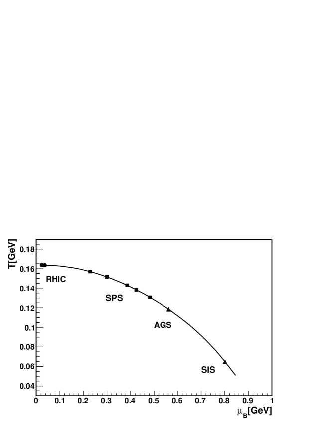
Figure 1: Chemical freeze-out curve for central Pb+Pb (Au+Au) collisions.

Once a suitable parameter set is determined, mean occupation numbers and fluctuations can be calculated using Eqs. (1) and  (2). The scaled variances of negative, positive, and all charged particles read:

$$\omega^{-}~{}=~{}\frac{\langle\left(\Delta N_{-}\right)^{2}\rangle}{\langle N_{-}\rangle}~{},~{}~{}~{}~{}\omega^{+}~{}=~{}\frac{\langle\left(\Delta N_{+}\right)^{2}\rangle}{\langle N_{+}\rangle}~{},~{}~{}~{}~{}\omega^{ch}~{}=~{}\frac{\langle\left(\Delta N_{ch}\right)^{2}\rangle}{\langle N_{ch}\rangle}~{},$$ (50)

where

$$\langle\left(\Delta N_{-}\right)^{2}\rangle~{} =~{}\sum_{i,j;~{}q_{i}<0,q_{j}<0}\langle\Delta N_{i}\Delta N_{j}\rangle~{},~{}~{}~{}~{}\langle\left(\Delta N_{+}\right)^{2}\rangle~{}=~{}\sum_{i,j;~{}q_{i}>0,q_{j}>0}\langle\Delta N_{i}\Delta N_{j}\rangle~{},$$ (51)

$$\langle\left(\Delta N_{ch}\right)^{2}\rangle~{} =~{}\sum_{i,j;~{}q_{i}\neq 0,q_{j}\neq 0}\langle\Delta N_{i}\Delta N_{j}\rangle~{}.$$ (52)

For the primordial hadrons, mean multiplicities, $\langle N_{i}\rangle$, in Eq. (50) are given by Eq.(4), and correlators, $\langle\Delta N_{i}\Delta N_{j}\rangle$, in Eqs. (51,52) are either the GCE or CE correlators from Eq. (15). For final state mean multiplicities, Eq. (45) is used, and correlators are calculated with Eq. (46) in the GCE or Eq. (III.3) in the CE, respectively. For final hadrons the summation needs to be extended to all stable particles with corresponding charges and all unstable resonances which have these charged particles in their decay channels. Figures 2, 3, and 4 show scaled variances for negatively charged particles, $\omega^{-}$, positively charged particles, $\omega^{+}$, and all charged particles, $\omega^{ch}$, respectively, as functions of $\sqrt{s_{NN}}$. Four cases are considered, namely, primordial and final state particles in both the GCE and CE. The relevant primordial and final state values for various colliding energies are summarized in Tables 2 and 3, respectively.

	$\omega^{ch}$		$\omega^{+}$		$\omega^{-}$
$\sqrt{s_{NN}}\left[GeV\right]$	GCE	CE	GCE	CE	GCE	CE
$2.32$	0.982	0.373	0.976	0.115	1.027	0.775
$4.86$	1.027	0.677	1.013	0.261	1.059	0.575
$6.27$	1.036	0.737	1.021	0.296	1.062	0.564
$7.62$	1.041	0.779	1.027	0.321	1.065	0.560
$8.77$	1.044	0.808	1.030	0.339	1.066	0.558
$12.3$	1.049	0.872	1.037	0.380	1.066	0.557
$17.3$	1.052	0.929	1.042	0.418	1.065	0.559
$130$	1.054	1.050	1.053	0.523	1.056	0.548
$200$	1.055	1.053	1.053	0.529	1.056	0.545

Table 2: Primordial scaled variances in the GCE and CE for central Pb+Pb (Au+Au) collisions.

	$\omega^{ch}$		$\omega^{+}$		$\omega^{-}$
$\sqrt{s_{NN}}\left[GeV\right]$	GCE	CE	GCE	CE	GCE	CE
$2.32$	1.048	0.403	1.020	0.116	1.025	0.777
$4.86$	1.354	0.848	1.195	0.327	1.058	0.621
$6.27$	1.421	0.967	1.201	0.395	1.068	0.643
$7.62$	1.464	1.059	1.198	0.449	1.076	0.668
$8.77$	1.491	1.124	1.194	0.486	1.082	0.687
$12.3$	1.542	1.268	1.182	0.571	1.095	0.732
$17.3$	1.576	1.387	1.171	0.643	1.105	0.770
$130$	1.619	1.613	1.138	0.802	1.128	0.824
$200$	1.620	1.617	1.136	0.808	1.130	0.822

Table 3: Final state scaled variances in the GCE and CE for central Pb+Pb (Au+Au) collisions.

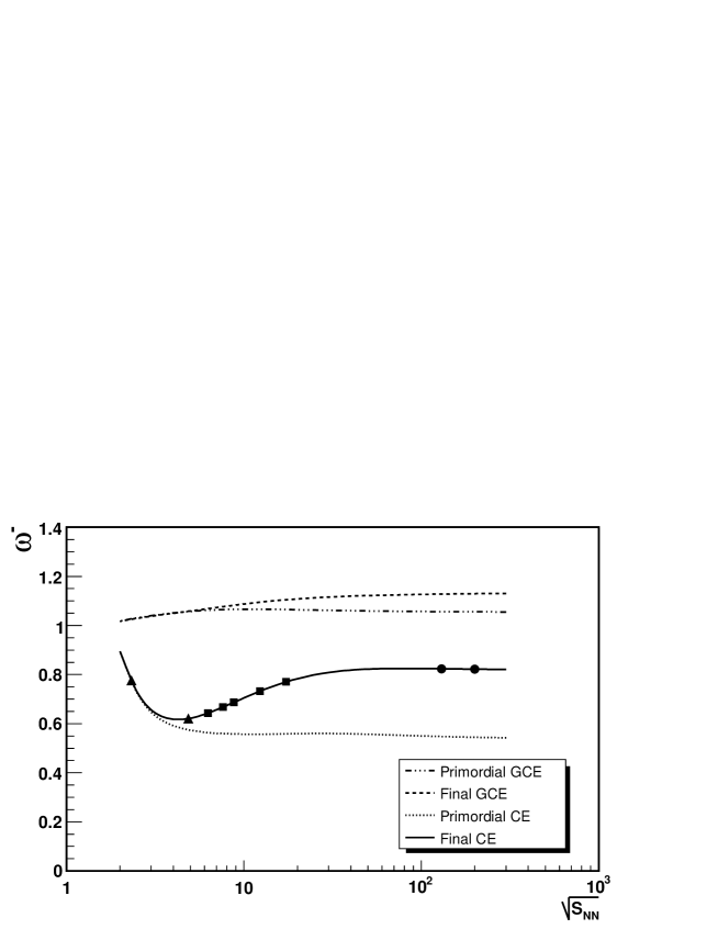
Figure 2: The scaled variances for negatively charged particles, $\omega^{-}$, along the chemical freeze-out line for central Pb+Pb (Au+Au) collisions (see Fig. 1). Different lines present primordial and final GCE and CE results.

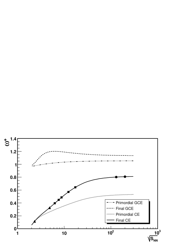
Figure 3: The scaled variances for positively charged particles, $\omega^{+}$, along the chemical freeze-out line for central Pb+Pb (Au+Au) collisions (see Fig. 1). Different lines present primordial and final GCE and CE results.

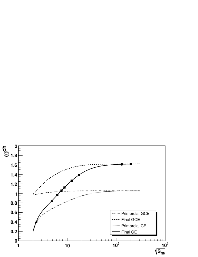
Figure 4: The scaled variances for all charged particles, $\omega^{ch}$, along the chemical freeze-out line for central Pb+Pb (Au+Au) collisions (see Fig. 1). Different lines present primordial and final GCE and CE results.

The column $\rho_{B}$ in Table I allows for a comparison with previously reported values of primordial scaled variances bec (a good agreement is found). The standard THERMUS particle table includes all strange and light flavored particles and resonances up to about $2.6$ GeV. Only strong and electromagnetic decays are considered, weakly decaying channels are omitted. It should be mentioned that, in particular, heavy resonances do not always have well established decay channels, thus there are always some ambiguities in the implementation of resonance decays in respective thermal model codes. Details about the THERMUS decay convention can be found in Ref. Thermus . The quoted values of the scaled variances are valid in the thermodynamic limit and assume that all charge carriers are detected. For high $\mu_{B}$ (low collision energies) the multiplicity of positively charged particles, $N_{+}$, is enhanced in a comparison with $N_{-}$, while the fluctuations $\omega^{+}$ are suppressed in a comparison with $\omega^{-}$. At vanishing net charge density (high collision energies), $\omega^{+}$ and $\omega^{-}$ have the same asymptotic values. The scaled variance for all charged particles $\omega^{ch}$ has the same value in the GCE and CE for a neutral system, for both primordial and final state. The effect of resonance decays remains small at low collision energies (i.e. small temperatures), while becoming sizeable even at the lowest SPS energy.

Some important qualitative effects are seen in Figs. 2, 3, and 4. The effect of Bose and Fermi statistics can be seen in primordial values in the GCE. At low temperatures Fermi statistics dominate, $\omega^{+}_{g.c.e.},\omega^{ch}_{g.c.e.}<1$, while at high temperature (low $\mu_{B}$) Bose statistics dominate, $\omega_{g.c.e.}^{\pm},\omega_{g.c.e.}^{ch}>1$. At the chemical freeze-out line, $\omega_{g.c.e.}^{-}$ is always slightly larger than 1, as $\pi^{-}$ is the dominant negative particle at low temperature too. A bump at small collision energies in $\omega^{+}_{g.c.e.}$ for final particles is due to the $\Delta^{++}$ decay into 2 positively charged hadrons, $p+\pi^{+}$. This single resonance contribution dominates at small collision energies (temperatures), but becomes relatively unimportant at high collision energies. A minimum in $\omega_{c.e.}^{-}$ for final particles is seen in Fig. 2. This happens as a result of the following effects. Since the number of negative particles is relatively small, $\langle N_{-}\rangle\ll\langle N_{+}\rangle$, at low collision energies, the CE suppression effects are also small. Low collision energies correspond to small temperatures of the hadron-resonance system, and the resonance decay effects are small too. With increasing $\sqrt{s_{NN}}$, the CE effects increase and this makes $\omega^{-}_{c.e}$ smaller, but resonance decay effects increase too and they work in an opposite direction making $\omega^{-}_{c.e}$ larger. A combination of these two effects, CE suppression and resonance enhancement, leads to a minimum structure of $\omega^{-}_{c.e}$ seen in Fig. 2.

The results for scaled variances presented in Figs. 2–4 and Tables II, III correspond to an ideal situation when all final hadrons are accepted by the detector. To compare our calculations to experimentally obtained values of $\omega$ the acceptance and resolution need to be taken into account. Observing only a fraction $q$ of final state particles dilutes the effect of global charge conservation. Even though the primordial particles at the chemical freeze-out line are only weakly correlated in the momentum space, this is no longer valid for final state particles as the decay products of resonances are not re-thermalized. Neglecting the momentum correlations due to resonance decays (this is approximately valid for $\omega^{+}$ and $\omega^{-}$, and much worse for $\omega^{ch}$) the following approximation for the scaled variances of experimentally accepted particles can be used (see e.g., ce-fluc ; fluc7 ),

$$\omega_{acc}~{}=~{}1~{}-~{}q~{}+~{}q~{}\omega_{4\pi}~{},$$ (53)

where $\omega_{4\pi}$ refers to an ideal detector with full $4\pi$-acceptance. In the limit of a very ‘bad’ (or ‘small’) detector, $q\rightarrow 0$, all scaled variances approach linearly to 1, i.e., this would lead to the Piossonian distributions for detected particles.

V Summary

The multiplicity fluctuations of hadrons in relativistic nucleus-nucleus collisions have been considered in the statistical model within the canonical ensemble formulation. The microscopic correlator method, previously used for one conserved charge, has been extended to include three conserved charges – baryon number, electric charge, and strangeness. The analytical formulae for the resonance decay contributions to the correlations and fluctuations have been found. Using the full hadron-resonance spectrum we have calculated the scaled variances of negative, positive and all charged particles for primordial and final hadrons at the chemical freeze-out in central Pb+Pb (Au+Au) collisions for different collision energies from SIS and AGS to SPS and RHIC. Both the CE and resonance decay effects for the multiplicity fluctuations have been discussed. A comparison with the NA49 data in Pb+Pb collisions at the SPS energies can be done for the sample of most central events with the number of projectile participants being close to its maximal value, $N_{P}^{proj}\approx A$, to avoid the fluctuations of the number of nucleon participants (see discussion in Ref. MGMG ; KGB ). These NA49 data will be available soon GL . The predictions of the statistical model within the CE formulations can be done for $\omega^{-}$ and $\omega^{+}$. In this case the experimental acceptance can be approximately introduced by a simple procedure based on Eq. (53). We find a qualitative difference between the CE results, $\omega^{\pm}_{c.e.}<1$, and the GCE ones, $\omega_{g.c.e.}^{\pm}>1$, for the accepted particles.

Appendix A

The n-dimensional Gauss integral equals the following korn :

$$\int_{-\infty}^{+\infty}\cdots\int_{-\infty}^{+\infty}\exp\left[\,-\sum_{i,\,k=1}^{n}A_{i,k}\,x_{i}x_{k}\,\right]dx_{1}\ldots dx_{n}\;=\;\frac{\pi^{n/2}}{|A|^{1/2}}\;,$$ (54)

where

$$|A|\;\equiv\;\det A\;=\;\sum_{i=1}^{n}(-1)^{i+k}A_{i,k}\,M_{i,k}~{},$$ (55)

and $M_{i,k}\;=\;(-1)^{i+k}\partial|A|/\partial A_{i,k}$ is a complementary minor of the element $A_{i,k}$. One also finds:

$$\int_{-\infty}^{+\infty}\cdots\int_{-\infty}^{+\infty}x_{i}x_{k}\;\exp\left[\,-\sum_{i,\,k=1}^{n}A_{i,k}\,x_{i}x_{k}\,\right]dx_{1}\ldots dx_{n}\;=\;\frac{\pi^{n/2}}{|A|^{3/2}}\;(-1)^{i+k}M_{i,k}\;.$$ (56)

References

- (1) J. Cleymans and H. Satz, Z. Phys. C 57, 135 (1993); J. Sollfrank, M. Gaździcki, U. Heinz, and J. Rafelski, ibid. 61, 659 (1994); G.D. Yen, M.I. Gorenstein, W. Greiner, and S.N. Yang, Phys. Rev. C 56, 2210 (1997); F. Becattini, M. Gaździcki, and J. Solfrank, Eur. Phys. J. C 5, 143 (1998); G.D. Yen and M.I. Gorenstein, Phys. Rev. C 59, 2788 (1999); P. Braun-Munzinger, I. Heppe and J. Stachel, Phys. Lett. B 465, 15 (1999); P. Braun-Munzinger, D. Magestro, K. Redlich, and J. Stachel, ibid. 518, 41 (2001); F. Becattini, M. Gaździcki, A. Keränen, J. Mannienen, and R. Stock, Phys. Rev. C 69, 024905 (2004).
- (2) J. Cleymans, H. Oeschler, K. Redlich, S. Wheaton, Phys. Rev. C 73, 034905 (2006).
- (3) F. Becattini, J. Manninen, M. Gaździcki, Phys. Rev. C 73, 044905 (2006).
- (4) P. Braun-Munzinger, K. Redlich, J. Stachel, nucl-th/0304013, Review for Quark Gluon Plasma 3, eds. R.C. Hwa and X.-N. Wang, World Scientific,Singapore.
- (5) R. Hagedorn, CERN Report 71-12 (1971); E.V. Shuryak, Phys. Lett. B 42, 357 (1972).
- (6) K. Redlich and L. Turko, Z. Phys. C 5, 541 (1980); J. Rafelski and M. Danos, Phys. Lett. B 97, 279 (1980) ; L. Turko, ibid B 104, 153 (1981); R. Hagedorn and K. Redlich, Z. Phys. C 27, 541 (1985); L. Turko and J. Rafelski, Eur. Phys. J. C 18, 587 (2001).
- (7) F. Becattini, Z. Phys. C 69, 485 (1996); F. Becattini, U. Heinz, ibid. 76, 269 (1997); F. Becattini, G. Passaleva, Eur. Phys. J. C 23, 551 (2002).
- (8) J. Cleymans, K Redlich, E. Suhonen, Z. Phys. C 51, 137 (1991); J. Cleymans, K Redlich, and E Suhonen, Z. Phys. C 58, 347 (1993); J. Cleymans, M. Marais, E. Suhonen, Phys. Rev. C 56, 2747 (1997); J. Cleymans, H. Oeschler, K. Redlich, Phys. Rev. C 59, 1663 (1999); Phys. Lett. B 485, 27 (2000); J.S. Hamieh, K. Redlich, and A. Tounsi, Phys. Lett. B 486, 61 (2000); J. Phys. G 27, 413 (2001); P. Braun-Munzinger, J. Cleymans, H. Oeschler, and K. Redlich, Nucl. Phys. A 697, 902 (2002); A. Tounsi, A. Mischke, and K. Redlich, Nucl. Phys. A 715, 565 (2003).
- (9) M.I. Gorenstein, M. Gaździcki, and W. Greiner, Phys. Lett. B 483, 60 (2000).
- (10) M.I. Gorenstein, A.P. Kostyuk, H. Stöcker, and W. Greiner, Phys. Lett. B 509, 277 (2001).
- (11) K. Werener and J. Aichelin, Phys. Rev. C 52, 1584 (1995); F. Liu, K. Werner and J. Aichelin, ibid 68, 024905 (2003); F. Liu, K. Werner, J. Aichelin, M. Bleicher, and H. Stöcker, J. Phys. G 30, S589 (2004); F. Becattini and L. Ferroni, Eur. Phys. J. C 35, 243(2004); ibid. 38, 225 (2004).
- (12) M. Gaździcki and St. Mrówczyński, Z. Phys. C 26, 127 (1992).
- (13) L. Stodolsky, Phys. Rev. Lett. 75, 1044 (1995); E.V. Shuryak, Phys. Lett. B 423, 9 (1998); St. Mrówczyński, Phys. Lett. B 430, 9 (1998).
- (14) G. Baym and H. Heiselberg, Phys. Lett. B 469, 7 (1999).
- (15) I.N. Mishustin, Phys. Rev. Lett. 82, 4779 (1999); Nucl. Phys. A 681, 56c (2001); H. Heiselberg and A.D. Jackson, Phys. Rev. C 63, 064904 (2001).
- (16) M.A. Stephanov, K. Rajagopal, and E.V. Shuryak, Phys. Rev. Lett. 81, 4816 (1998); M.A. Stephanov, Acta Phys. Polon. B 35, 2939 (2004).
- (17) M.A. Stephanov, K. Rajagopal, and E.V. Shuryak, Phys. Rev. D 60, 114028 (1999).
- (18) S. Jeon and V. Koch, Phys. Rev. Lett. 83, 5435 (1999).
- (19) S. Jeon and V. Koch, Phys. Rev. Lett. 85, 2076 (2000).
- (20) H. Heiselberg, Phys. Rep. 351, 161 (2001).
- (21) S. Jeon and V. Koch, hep-ph/0304012, Review for Quark-Gluon Plasma 3, eds. R.C. Hwa and X.-N. Wang, World Scientific, Singapore.
- (22) M. Bleicher et al., Nucl. Phys. A 638, 391 (1998); Phys. Lett. B 435, 9 (1998); Phys. Rev. C 62, 061902 (2000); ibid. 62, 041901 (2000); S. Jeon, L. Shi, and M. Bleicher, nucl-th/0506025; S. Haussler, H. Stoecker, and M. Bleicher, hep-ph/0507189.
- (23) M. Gaździcki, M.I. Gorenstein, and St. Mrówczyński, Phys. Lett. B 585, 115 (2004); M.I. Gorenstein, M. Gaździcki, and O.S. Zozulya, ibid. 585, 237 (2004); M. Gaździcki, nucl-ex/0507017.
- (24) M. Gaździcki and M.I. Gorenstein, hep-ph/0511058.
- (25) V.P. Konchakovski, S. Haussler, M.I. Gorenstein, E.L. Bratkovskaya, M. Bleicher, and H. Stöcker, Phys. Rev. C 73, 034902 (2006).
- (26) V.V. Begun, M. Gaździcki, M.I. Gorenstein, and O.S. Zozulya, Phys. Rev. C 70, 034901 (2004).
- (27) V.V. Begun, M.I. Gorenstein, and O.S. Zozulya, Phys. Rev. C 72, 014902 (2005).
- (28) A. Keränen, F. Becattini, V.V. Begun, M.I. Gorenstein, and O.S. Zozulya, J. Phys. G 31, S1095 (2005).
- (29) F. Becattini, A. Keränen, L. Ferroni, T. Gabbriellini, Phys. Rev. C 72, 064904 (2005).
- (30) V.V. Begun and M.I. Gorenstein, Phys. Rev. C 73, 054904 (2006).
- (31) V.V. Begun, M.I. Gorenstein, A.P. Kostyuk, and O.S. Zozulya, Phys. Rev. C 71, 054904 (2005).
- (32) V.V. Begun, M.I. Gorenstein, A.P. Kostyuk, and O.S. Zozulya, J. Phys. G 32, 935 (2006).
- (33) J. Cleymans, K. Redlich, L. Turko, Phys. Rev. C 71, 047902 (2005); J. Phys. G 31, 1421 (2005).
- (34) M. Hauer, Master Thesis, Cape Town University, South Africa.
- (35) L.D. Landau and E.M. Lifschitz, Statistical Physics (Fizmatlit, Moscow, 2001).
- (36) G. Torrieri, S. Steinke, W. Broniowski, W. Florkowski, J. Letessier and J. Rafelski, Comput. Phys. Commun. 167 (2005) 229.
- (37) S. Wheaton, J. Cleymans, J. Phys. G 31 1069-1074 (2005).
- (38) J. Cleymans and K. Redlich, Phys. Rev. Lett. 81, 5284 (1998).
- (39) M. Gaździcki and B. Lungwitz, private communications.
- (40) G.A. Korn and T.M. Korn, Mathematical Handbook (MGRAW-HILL, New York, 1961).