Isospin fractionation : equilibrium versus spinodal decomposition

Abstract

This paper focuses on the isospin properties of the asymmetric nuclear-matter liquid-gas phase transition analyzed in a mean-field approach, using Skyrme effective interactions. We compare two different mechanisms of phase separation for low-density matter: equilibrium and spinodal decomposition. The isospin properties of the phases are deduced from the free-energy curvature, which contains information both on the average isospin content and on the system fluctuations. Some implications on experimentally accessible isospin observables are presented.

I Introduction

The nuclear interaction is a mean-range attractive, short-range repulsive force. Because of this, nuclear matter is expected to present a phase transition of the liquid-gas type Finn ; Bertsch . The nuclear-matter phase diagram has been studied in detail in the case of symmetric matter, i.e. a system with the same number of protons and neutrons Das-PhysRep . The case of asymmetric matter involves an additional degree of freedom, isospin. As a result, its study is more complex and allows to observe specific effects such as the phenomenon of isospin fractionation Xu . The knowledge of these properties is of great interest for the physics of neutron-rich systems. Such systems have become the subject of many investigations in the recent nuclear-physics literature. Exotic-nucleus transport properties and multifragmentation are expected to provide constraints on the nuclear equation of state, in particular on the density dependence of the symmetry energy Baran-PhysRep410 ; Tsang ; Ono . In astrophysics, both neutron-star structure and supernova dynamics are influenced by phase transitions of neutron-rich matter in a large interval of temperatures and densities Lattimer-PhysRep ; Glendenning . All these different phenomena involve excited matter at baryon densities lower than normal nuclear matter density : this corresponds in the phase diagram to a region of instability with respect to phase separation. In the case of neutron-star crusts the system lifetime is such that one can safely modelize phase separation in terms of equilibrium. However this is not the case for exploding supernova cores, and even less for heavy-ion collisions. For such systems with a finite lifetime, the out-of-equilibrium phenomenon of spinodal decomposition may be the leading mechanism for phase separation Chomaz-PhysRep .

For the work presented in this paper, we have studied nuclear matter in a mean-field approach, using Skyrme effective interactions. Three different parameterizations are used. The more recent one, Sly230a Chabanat , is used as a reference since it has been fitted to exotic nuclei and neutron-matter properties, which makes it particularly well-adapted to the description of neutron-rich matter. Two others are used as a comparison : SGII SGII , which has been shown to reproduce isospin effects studied through giant dipole resonances Catara-NPA624 , and SIII SIII , which is one of the first Skyrme parametrizations and is not constrained for asymmetric matter. Contrary to Sly230a and SGII, SIII is certainly not a realistic parameterization; we have included it in our comparison since it is still used in some transport codes because of its simplicity Baran-PhysRep410 .

In section II, we present the phase diagram of nuclear matter, which is a representation of phase separation at equilibrium. Then the phase properties are considered, comparing the case of equilibrium and spinodal decomposition. In section III, we study the direction of phase separation, leading to the phenomenon of isospin fractionation. The consequences of our findings on the possible extraction of the symmetry-energy coefficient from isoscaling data Tsang ; Ono are explored in section IV. In section V we discuss fluctuations in the system isotopic composition.

II Phase diagram

Gibbs statistical equilibrium is defined by the maximization of the system Shannon entropy $S=-Tr(\hat{D}log\hat{D})$, where $\hat{D}$ is the many-body density matrix of the system Balian . Let us consider $S$ represented for a homogeneous system in the space of observables. If $S$ presents a convexity in this representation, it can be maximized by phase mixing, which corresponds to a linear interpolation between two points of the space of observables. The coexistence region is then defined as the ensemble of points for which entropy can be enhanced by such an interpolation. If the system is located at a given point inside coexistence region, there is a unique decomposition in a couple of two other points that gives the best maximization of entropy : they define the two phases at equilibrium. This couple is determined by Gibbs construction Huang , which consists in building the concave envelope of the entropy surface by linear interpolation in the space of observables : phases at equilibrium then belong to the same tangential plane Muller-Serot ; Glendenning .

This geometrical condition results in the well-known equality of all intensive parameters. Let us consider a system occupying a volume $V$ described by a set of observable densities $\{a_{k}\}=\{\langle\hat{A}_{k}\rangle/V\}$ controlled by the associated intensive parameters $\{\lambda_{k}\}$, related to the entropy density $s=S/V$ by :

$$\lambda_{l}=\partial_{a_{l}}s(\{a_{k}\})$$ (1)

The pressure $P$ is related to the entropy by :

$$\beta P=s-\sum_{k}\lambda_{k}a_{k}$$ (2)

Let us now consider two points of the space of observables $\{a_{k}\}^{(1)}$ and $\{a_{k}\}^{(2)}$. Entropy has the same tangent plane at these two points if $\{\lambda_{k}\}^{(1)}=\{\lambda_{k}\}^{(2)}$ (equality of plane slopes) and $P^{(1)}=P^{(2)}$ (equality of plane origins) : these are Gibbs equilibrium conditions on the intensive parameters.

In the case of asymmetric nuclear matter, the relevant observables are neutron, proton and energy densities, $\{a_{k}\}=\{\rho_{n},\rho_{p},e\}$; the associated intensive parameters are $\{\lambda_{k}\}=\{-\beta\mu_{n},-\beta\mu_{p},\beta\}$ where $\mu_{q}$ $(q=n,p)$ are the chemical potentials and $\beta$ is the inverse temperature. To obtain the phase diagram of nuclear matter, expressions linking observables and the associated intensive parameters (i.e. equations of states) are needed. We have worked out such relations in the mean-field approach Ducoin .

Let us first express the average energy density of homogeneous nuclear matter, $e=\langle\hat{H}\rangle/V$. With a Skyrme effective interaction, $e$ is a functional of one-body densities only: particle densities $\rho_{q}$ and kinetic densities $\tau_{q}=\langle\hat{P}^{2}\rangle_{q}/\hbar^{2}V$. We introduce isoscalar and isovector densities :

$$\begin{array}[]{ll}\rho=\rho_{n}+\rho_{p}\;,&\;\tau=\tau_{n}+\tau_{p}\\ \rho_{3}=\rho_{n}-\rho_{p}\;,&\;\tau_{3}=\tau_{n}-\tau_{p}\end{array}$$ (3)

In the case of homogeneous, spin-saturated matter with no Coulomb interaction, the energy density can be written as :

$$e=\frac{\hbar^{2}}{2m}\tau+C_{0}\rho^{2}+D_{0}\rho_{3}^{2}+C_{3}\rho^{\sigma+2}+D_{3}\rho^{\sigma}\rho_{3}^{2}+C_{eff}\rho\tau+D_{eff}\rho_{3}\tau_{3}$$ (4)

where coefficients $C_{i}$ an $D_{i}$ are linear combinations of the standard Skyrme parameters Chabanat ; Ducoin

$$\begin{array}[]{ll}C_{0}&=\ \ 3t_{0}/8\\ D_{0}&=-t_{0}(2x_{0}+1)/8\\ C_{3}&=\ \ t_{3}/16\\ D_{3}&=-t_{3}(2x_{3}+1)/48\\ C_{eff}&=\ \ [3t_{1}+t_{2}(4x_{2}+5)]/16\\ D_{eff}&=\ \ [t_{2}(2x_{2}+1)-t_{1}(2x_{1}+1)]/16\end{array}$$

.

Mean-field approaches describe nucleons as independent particles. Each particle of type $q$ is submitted to the mean field $\hat{W}_{q}$ defined by the relation $\delta\langle\hat{H}\rangle=Tr(\hat{W}_{q}\delta\hat{\rho_{q}})$, where $\delta\hat{\rho_{q}}$ represents any variation of the one-body density matrix associated with the particle $q$, leading to the expression :

$$\hat{W}_{q}=\frac{\partial e}{\partial\tau_{q}}\frac{\hat{p}^{2}}{\hbar^{2}}+\frac{\partial e}{\partial\rho_{q}}=\frac{1}{2m_{q}^{*}}\hat{p}^{2}+U_{q}$$ (5)

The mean field is composed of a potential term $U_{q}=\partial_{\rho_{q}}e$, and a kinetic term involving an effective mass $m_{q}^{*}$ defined by $\hbar^{2}/2m_{q}^{*}=\partial_{\tau_{q}}e$.

This determines individual energy levels $\epsilon_{q}^{i}=\frac{p_{i}^{2}}{2m_{q}^{*}}+U_{q}$ with the usual quantification conditions on the momenta provided by the boundary conditions. In the grand-canonical approach, for a given temperature $T=\beta^{-1}$, these levels are occupied according to Fermi-Dirac statistics :

$$n_{q}(p)=1/\left[1+exp(\beta(p^{2}/2m_{q}^{*}+U_{q}-\mu_{q})\right]$$ (6)

where $\mu_{q}$ is the chemical potential of the particles of type $q$ .

All one-body densities are then given by Fermi integrals. In particular the independent-particle partition sum can be expressed in the same way as for an ideal gas:

$$\frac{\ln Z_{0}}{V}=2\sum_{q}\int_{0}^{\infty}\ln(1+e^{-\beta(\frac{p^{2}}{2m_{q}^{*}}-\mu_{q}^{\prime})})\frac{4\pi p^{2}}{h^{3}}dp=\sum_{q}\frac{\hbar^{2}}{3m_{q}^{*}}\beta\tau_{q}$$ (7)

where $\mu_{q}^{\prime}=\mu_{q}-U_{q}$. At this point it is important to recall that the independent particle partition sum $Z_{0}$ should not be confused with the mean-field grand-canonical partition sum which is related to the mean-field pressure $\log Z=\beta PV$ and can be computed from the mean-field entropy using $\log Z=S-\beta(<\hat{H}>-\mu_{p}<\hat{N}_{p}>-\mu_{n}<\hat{N}_{n}>)$.

For fixed values of $\rho_{n}$ and $\rho_{p}$ at a given temperature, chemical potentials are obtained by iteratively solving the self-consistent relations between $\rho_{q}$, $\mu_{q}$ and $m_{q}^{*}$. We can then compute the kinetic density and calculate the entropy as a function of densities. Indeed, the mean-field solution comes from a variational approximation to the entropy so the mean-field entropy $S_{0}$ provides the best independent-particle approximation to the exact entropy. The mean-field entropy can easily be derived from the independent-particle partition sum and the average of the mean-field potential $\langle\hat{W}\rangle_{0}$ so we get Vautherin :

$$S/V\simeq S_{0}/V=\ln Z_{0}/V+\beta(\langle\hat{W}\rangle_{0}/V-\mu_{n}\rho_{n}-\mu_{p}\rho_{p})$$ (8)

which gives for a fixed $\beta$ the entropy $s=S/V$ as a function of neutron and proton densities.

As we have already mentioned, the construction of the concave envelope of $s(e,\rho_{n},\rho_{p})$ implies Gibbs conditions for each couple of phases at equilibrium : $\beta^{(1)}=\beta^{(2)}$, $\mu_{n}^{(1)}=\mu_{n}^{(2)}$, $\mu_{p}^{(1)}=\mu_{p}^{(2)}$ and $P^{(1)}=P^{(2)}$. Let us now introduce the constrained entropy defined by

$$s_{c}=-\beta f=s-\beta e.$$ (9)

which corresponds to the opposite of the free energy $f$, divided by the temperature. Gibbs construction can then be performed by constructing the concave envelope of $s_{c}$ in $(\rho_{n},\rho_{p})$ plane at a fixed temperature $T=\beta^{-1}$. Indeed, $\beta$ is imposed to be constant, and the definition of $s_{c}$ ensures that its tangent-plane slopes and altitude give respectively the chemical potentials and the pressure :

$$\left(\partial_{\rho_{q}}s_{c}(\rho_{n},\rho_{p})\right)_{\beta}=\partial_{\rho_{q}}s(e,\rho_{n},\rho_{p})=-\beta\mu_{q}$$ (10)

$$s_{c}+\beta(\mu_{n}\rho_{n}+\mu_{p}\rho_{p})=s-\beta(e-\mu_{n}\rho_{n}-\mu_{p}\rho_{p})=\beta P$$ (11)

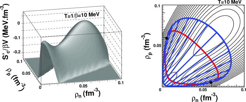
Figure 1: Constrained entropy at $T=10MeV$, corrected by $\beta\mu_{s}\rho$ in order to emphasize curvature properties. It is shown on the left in perspective, and on the right as a contour plot. On the right, coexistence and spinodal boundaries are added as thick lines. Outer curve: coexistence. Straight lines link selected couples of phases at equilibrium. Inner curve: spinodal. Dots: critical points.

The introduction of the constrained entropy permits then to reduce the dimensionality of the problem since we can work at constant temperature. The constrained entropy is represented in fig.1, at a temperature of $10$ MeV. In this figure, a slope has been subtracted in order to emphasize curvature properties: the surface represented is $s^{\prime}_{c}=s_{c}+\beta\mu_{s}\rho$, where $\mu_{s}$ is the chemical potential of symmetric matter at the transition. The constrained entropy is symmetric with respect to the axis $\rho_{n}=\rho_{p}$, reflecting the invariance of nuclear interaction with respect to neutron-proton exchange.

We observe that the surface obtained presents a region of positive convexity : this is the case if we fix any temperature under the critical temperature of symmetric matter, which is, in the Sly230a parameterization, $T_{c}=14.54MeV$ (for comparison, we get $T_{c}=14.46MeV$ with SGII and $17.96MeV$ with SIII). The concave-envelope construction performed on this surface links couples of phases at equilibrium. The ensemble of these points forms the two branches of the coexistence curve, one at lower density (gas) and the other at higher density (liquid). They join at two critical points, where the difference between the two phases disappears.

The coexistence curve is the boundary of the coexistence region, inside which a system at equilibrium is decomposed into two phases situated on each branch. The region presenting a positive convexity is the spinodal region. In this region, infinitesimal density fluctuations may lead to an increase of entropy. The system is locally unstable. The spinodal region is by construction inside coexistence. Coexistence and spinodal boundaries are tangent at the critical points. These curves are represented on the right part of fig.1.

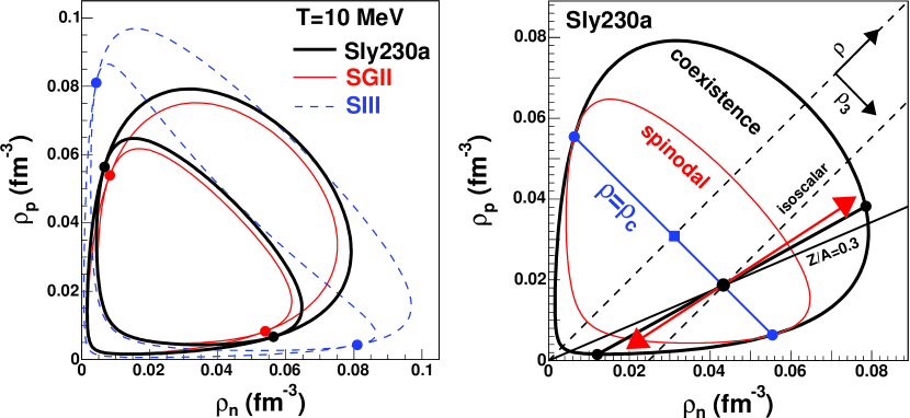
Figure 2: Coexistence and spinodal curve in the density plane at $T=10MeV$. Left: comparison between different Skyrme parameterizations : Sly230a (thick lines), SGII (thin lines) and SIII (dashed lines). Right: illustration of phase separation for a system of proton fraction $Z/A=0.3$ inside instability region (cf section III).

The phase diagram of the three different Skyrme forces is compared for the same temperature $T=10$ MeV on the left part of fig.2. Sly230a and SGII give close results, while SIII shows an atypical behaviour, especially, as expected, on the asymmetric parts of the diagram.

III Direction of phase separation

Let us consider a system whose proton fraction $Z/A$ and total density $\rho$ are such that it is situated inside instability region. This is illustrated on the right-hand side of fig.2 for a neutron-rich system ($Z/A=0.3$).

If equilibrium is reached, this system will undergo phase separation according to Gibbs construction. We can see that the corresponding phases in coexistence, represented as black dots on the coexistence border on the right part of fig.2, do not belong to the line of constant proton fraction. We can remark that the liquid fraction is closer to symmetric matter than the gas fraction: this behavior is a consequence of the symmetry-energy minimization in the dense phase. This inequal repartition of isospin between the two phases is the well-known phenomenon of isospin fractionation Muller-Serot .

In order to quantify the phenomenon of isospin fractionation, we will study the associated directions in the density plane. The line of constant proton fraction defines a direction $\mathbf{u}_{Z/A}$. Let us introduce the isoscalar direction $\mathbf{u}_{\rho}$, which corresponds to the axis of total density $\rho=\rho_{n}+\rho_{p}$. The equilibrium direction $\mathbf{u}_{eq}$ is given by the straight line that joins the couple of phases in coexistence. Isospin fractionation is linked to the difference between $\mathbf{u}_{eq}$ and $\mathbf{u}_{Z/A}$. The equilibrium direction being rotated towards $\mathbf{u}_{\rho}$, phase separation gives a liquid more asymmetric than the gas.

We now turn to study isospin fractionation if phase separation occurs out of equilibrium. Specifically, if the system is brought inside the spinodal region in a reaction too fast for global equilibrium to be achieved, its evolution will be driven by local instabilities instead of global Gibbs construction. This is spinodal decomposition Chomaz-PhysRep : the local properties of the constrained entropy curvature determine the development of a spinodal instability into phase separation. The information for this study is contained in the free-energy curvature matrix given by :

$$C=\left(\begin{array}[]{ll}\partial^{2}f/\partial\rho_{n}^{2}&\partial^{2}f/\partial\rho_{n}\partial\rho_{p}\\ \partial^{2}f/\partial\rho_{p}\partial\rho_{n}&\partial^{2}f/\partial\rho_{p}^{2}\\ \end{array}\right)=\left(\begin{array}[]{ll}\partial\mu_{n}/\partial\rho_{n}&\partial\mu_{p}/\partial\rho_{n}\\ \partial\mu_{n}/\partial\rho_{p}&\partial\mu_{p}/\partial\rho_{p}\\ \end{array}\right)$$ (12)

This matrix is defined for each point of the density plane. The lower eigen-value $C_{<}$ corresponds to the minimal curvature of $f$ at the considered point. The spinodal border is the ensemble of points for which $C_{<}=0$. The instability region is defined by $C_{<}<0$ : in such points, there are directions of abnormal curvature, corresponding to a concave free energy. The eigen-vetctor $\mathbf{u}_{<}$ associated with the lower eigen-value gives the direction of most negative curvature: this is the instability direction. It is represented by the double arrow on the example of fig.2, where we can see that spinodal decomposition leads to a more pronounced fractionation than equilibrium, the denser phase getting closer to the symmetric matter. It is important to remark at this point that the instability direction does not give a direct quantitative measurement of the final fractionation after phase separation. For this to be true, the effect of the evolution of density fluctuations on the isospin composition has to be completely neglected. If this is certainly an approximation ColonnaMatera , it has been however shown in explicit transport calculations Chomaz-PhysRep that the initial instability largely dominates the subsequent dynamics. The interest of employing this simplified approach as complementary to more sophisticated transport codes is that, within this approximation, the spinodal mechanism can be directly compared to phase separation at equilibrium. Indeed the equilibrium direction can also be expressed as the eigen-vector of a curvature matrix, like the instability direction. Let us define $f^{eq}$ as the free energy at equilibrium, i.e. after correction of the curvature anomaly by phase mixing according to Gibbs construction. This construction imposes a positive curvature at each point, and a zero curvature between two phases in coexistence. As a result, in the coexistence region the lower eigen-value of the $f^{eq}$ curvature matrix is zero, and the associated eigen-vector is what we have defined as the equilibrium direction, $\mathbf{u}_{eq}$. In the following, we will denote $f^{0}$ and $f^{eq}$ the free energy before and after Gibbs construction, their respective curvature eigen-modes being $(C_{<}^{0},\mathbf{u}_{<}^{0},C_{>}^{0},\mathbf{u}_{>}^{0})$ and $(C_{<}^{eq},\mathbf{u}_{<}^{eq},C_{>}^{eq},\mathbf{u}_{>}^{eq})$. A qualitative impression of how equilibrium and instability directions compare through the density plane can be gained from fig.3 for the three Skyrme forces. In order to follow the eigen-direction of the curvature matrix, we draw curves which are everywhere tangential to the curvature eigenvectors. Both directions of phase separation at equilibrium (Gibbs construction) and out of equilibrium (spinodal decomposition) remain quite close, and essentially isoscalar Margueron-isoscalar ; Baran-PhysRep410 . A comparable degree of isospin fractionation, with formation of a more symmetric liquid, is conserved all through the instability region. The dominant feature is that the instability direction leads to more fractionation than equilibrium.

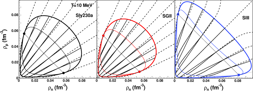
Figure 3: Global representation of phase-separation directions through the density plane, for three different Skyrme parameterizations. Coexistence and spinodal boundaries are represented as in fig.2. A few selected equilibrium directions are given by straight lines joining the high and low-density branches of the coexistence curve (these straight lines are everywhere tangent to the equilibrium direction $\mathbf{u}_{<}^{eq}$). Phase-separation directions in spinodal decomposition are represented by a selection of lines which are everywhere tangent to the instability direction $\mathbf{u}_{<}^{0}$. They are drawn as full lines inside the spinodal region where they correspond to an instability direction, and prolongated in dashed lines ouside the spinodal, where there is no more local instability.

In order to have a quantitative comparison of the different fractionations, it is convenient to express the directions of phase separation as slopes with respect to the isoscalar direction $\delta\rho_{3}/\delta\rho$. This quantity gives a measure of the degree of fractionation associated with phase separation. It can in principle vary from zero (in the case of a purely isoscalar phase separation), to infinity (in the case of a purely isovector instability, corresponding to a separation of protons from neutrons into two phases at the same baryon density). In practice $\delta\rho_{3}/\delta\rho$ is always a small number Margueron-isoscalar ; Baran-PhysRep410 . This is easy to understand considering that i) proton and neutron kinetic energies favour equal-size Fermi spheres and ii) the nuclear interaction is more attractive in the proton-neutron than the proton-proton and neutron-neutron channels in any realistic nuclear physics model ($T=0$ contribution), which favours the existence of a mixed isospin bound phase.

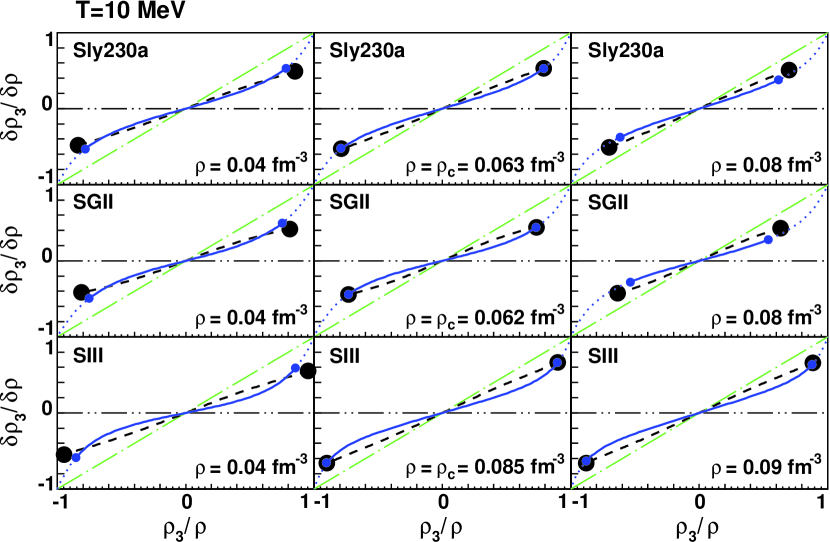
Figure 4: Phase-separation directions $\delta\rho_{3}/\delta\rho$ at equilibrium (dash) and in spinodal decomposition (solid) as a function of the asymmetry $\rho_{3}/\rho$ for three different Skyrme parameterizations at different values of $\rho$ : below, at and above the associated critical density. The instability direction is continued by the lowest curvature direction (dotted line). The dot-dash straight line gives the direction of constant $Z/A$ while the double-dot-dash horizontal line gives the isoscalar direction $\delta\rho_{3}=0$. Small dots give spinodal boundaries and large ones coexistence region boundaries.

The evolution of $\delta\rho_{3}/\delta\rho$ (degree of fractionation) with $\rho_{3}/\rho$ (system asymmetry) is given by fig.4 for three different total densities : below, at, and above the respective critical density $\rho_{c}$ (i.e the total density at critical points). In this representation, the direction of constant proton fraction is a diagonal straight line while the isoscalar direction is an horizontal line. On this figure, equilibrium and instability direction are compared for the different Skyrme parameterizations.

Phase-separation evolutions verify some expected constraints. First, the isospin invariance of Skyrme interactions ensures that the graphs are symmetric with respect to $\rho_{3}=0$. It also imposes that all directions become purely isoscalar in the case of symmetric matter, i.e. all curves must join at the origin $(\delta\rho_{3}/\delta\rho,\rho_{3}/\rho)=(0,0)$. Another constraint is given by the ending points of the curves. At these borders ($|\rho_{3}|=\rho$), the vanishing of one species means that its chemical potential at finite temperature goes to $-\infty$, implying an infinite curvature of the free energy in the corresponding direction. The minimal curvature $\mathbf{u}_{<}^{0}$ is then oriented along the axis of the remaining species, which is also the direction of constant $Z/A$.

The first observation is that spinodal and phase-equilibrium directions are very close and lie between the isoscalar direction and the constant-proton-fraction one. This means that they lead to a rather similar fractionation. In order to get a deeper insight, let us consider the various densities in more details.

Let us consider the case of the axis at $\rho=\rho_{c}$, for which the instability region ends at the critical points. Between these extremities, the instability direction induces more fractionation than equilibrium since it is closer to isoscalar direction. At the critical points, where the spinodal and coexistence curves are tangent, both directions of phase separation join to become tangential to the coexistence and spinodal borders. This is an additional constraint on phase-separation directions which, with the already discussed constraints, explains the similarities between the phase-separation directions at and out of equilibrium. This additional constraint does not apply if the total density we consider is not $\rho_{c}$. We observe that for $\rho<\rho_{c}$, a small inversion occurs around the extremities of the instability region. For $\rho>\rho_{c}$ instead, a phase separation out of equilibrium induces more fractionation for all isospin asymmetries.

These observations stand for the three Skyrme forces that we have considered. The quantitative differences, which essentially distinguish SIII from the two more recent parameterizations, do not affect the qualitative features that have been described. This is partly due to the above discussed constraints.

IV Fractionation and isocaling observables

In a variety of experimental situations, it has been observed that the isotopic-yield ratio for two reactions (denoted $(1)$ and $(2)$) of different asymmetry approximatly follows an exponential form Tsang :

$$R_{iso}^{(1),(2)}(N,Z)=Y^{(2)}(N,Z)/Y^{(1)}(N,Z)\propto exp(\alpha_{n}N+\alpha_{p}Z).$$ (13)

This phenomenon is known under the name of isoscaling. In an equilibrium interpretation in the grand-canonical ensemble, the isoscaling parameters $\alpha_{q}$ should be linked to the chemical potentials and temperature of the systems, $\alpha_{q}=(\mu_{q}^{(2)}-\mu_{q}^{(1)})/T$. It has been proposed to extract from the measured isoscaling parameters the symmetry-energy coefficient $C_{sym}$ through the approximate formula Ono ; Shetty :

$$\alpha_{n}=4C_{sym}([Z/\langle A\rangle]_{(1)}^{2}-[Z/\langle A\rangle]_{(2)}^{2})/T.$$ (14)

This relation, derived for the grand-canonical ensemble in the saddle-point approximation Ono , holds in the hypothesis of equilibrium at the time of fragment formation. This means that to extract $C_{sym}(Z)$ from the measured isoscaling parameters, modifications of $\alpha_{n}$ due to secondary decay have to be accounted for and the proton fraction of the most probable isobar for each $Z$ should be known at the time of fragment formation .

Because of the small variation of $\alpha_{n}$ with the atomic number, an average estimation of $C_{sym}$ can be obtained using for $[Z/\langle A\rangle]_{(i)}$ the average proton content of the liquid fraction Ono . Since even this quantity is not experimentally known, a similar formula can be found in the literature, where, however, the proton fraction of the fragmenting source $[Z_{0}/A_{0}]_{(i)}$ is used instead of $[Z/\langle A\rangle]_{(i)}$: this leads to a quantity we call $C_{sym}^{0}$ Tsang2 ; LeFevre ; Botvina . This approximation is supported by the fact that in the zero-temperature limit the proton fraction of the fragments converges to the proton fraction of the source Botvina .

However, in general this does not need to be the case and the approximated $C_{sym}^{0}$ may differ from the value $C_{sym}$. In particular, both in the equilibrium hypothesis at finite temperature and in the case of dynamical fragment formation through spinodal decomposition, as we have seen, we can expect the phenomenon of fractionation: fragments should not have the same isospin ratio as the fragmenting source. This should affect the value of $C_{sym}$ obtained from the isoscaling coefficients.

Our equilibrium nuclear-matter approach does not allow to give quantitative predictions on the actual isospin content of fragments obtained out of the different phase-separation mechanisms; we can however make some qualitative order of magnitude estimations of the possible deformation that isospin fractionation may induce on symmetry-energy measurements.

Dynamical transport models Baran-PhysRep410 ; Ono indicate that clusterization takes place at a relatively well-defined density inside the spinodal region determined by the collision dynamics and corresponding to the first development of instabilities, for which we take a typical value around $\rho_{0}/3$. Spinodal decomposition is then a phenomenon fast enough for fragment formation dynamics to be dominated by the amplification of the most unstable modes at this density Chomaz-PhysRep . This density then determines the phase-separation direction.

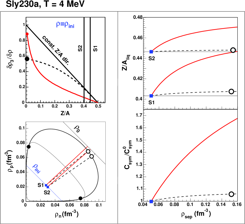
Figure 5: Influence of isospin fractionation on $C_{sym}$ measurement at $T=4MeV$. Left side: phase-separation directions. Top-left: separation direction at a typical density of fragment formation $\rho=\rho_{ini}=0.05fm^{-3}$, as a function of the global proton fraction for equilibrium (dashed line) and spinodal instability (full line). Vertical lines indicate the two systems S1$\sim$¹¹²Sn, S2$\sim$¹²⁴Sn. Bottom-left: representation of the corresponding phase separations in the density plane. Right side: consequence on symmetry-energy measurement. Top-right : average isotopic composition of the liquid-like fraction as a function of fragment density at separation, for the two systems S1 and S2. Bottom-right: Symmetry energy coefficient $C_{sym}$ compared to the approximate expression obtained neglecting fractionation $C_{sym}^{0}$, as a function of separation density, for equilibrium (dashed line) and spinodal instability (full line). In the case of equilibrium, the liquid position is fixed in the density plane: it is indicated by the empty circles.

The left part of fig.5 displays, similar to fig.4 above, the directions of phase equilibrium and spinodal decomposition as a function of Z/A at a typical temperature of $T=4MeV$. The case of two systems with global proton fractions corresponding to ¹¹²Sn and ¹²⁴Sn is shown by the vertical lines. We can see that fractionation at equilibrium is negligible in agreement with ref.Botvina , and fragmentation of more exotic nuclei should be studied to explore this effect. However even for these stable systems, spinodal decomposition gives an important fractionation, and the effect would be amplified using more asymmetric systems.

Once the direction of phase separation is known, the final composition of the fragments depends only on their density at freeze-out, when they become separated. We call this density $\rho_{sep}$. The average $Z/A$ of the liquid fraction is represented in the central part of fig.5 as a function of the density at separation. This density must be between the initial density and the saturation value, but its actual value is not known from fundamental principles. It is generally assumed that fragments at separation are at normal density $\rho_{sep}\approx\rho_{0}$. Recent AMD calculations however seem to indicate that lower values $\rho\approx 0.1fm^{-3}$ may be more realistic Shetty ; Ono2 .

The asymmetry coefficient $C_{sym}$ deduced through eq.(14) is compared to its approximate value $C_{sym}^{0}$ obtained with the proton fraction of the fragmenting source in the right part of fig.5. Little change (few % at maximum) is observed in the case of equilibrium, again consistently with the predictions of the statistical model Botvina . However, the stronger fractionation effect in the case of spinodal decomposition sensitively decreases, by up to $50\%$ (or more), the approximate asymmetry coefficient. This implies that the low values reported for $C_{sym}$ in ref.LeFevre may be alternatively interpreted as a signal of isospin fractionation in a spinodal decomposition.

V Isospin fluctuations

In section III, we have studied the direction of phase separation, corresponding to the direction of minimal curvature of the free energy $\mathbf{u}_{<}$. This direction can be qualitatively linked to the average isospin content of fragments issuing from the phase-separation mechanism. As we have seen in section IV, some quantitative predictions can also be obtained if some extra hypotheses are made, namely that fragment-formation dynamics is dominated by an amplification of instabilities from well-defined initial density and temperature. Within the same line of reasoning, the other eigen-vector $\mathbf{u}_{>}$ giving the direction of maximal curvature can be linked to fluctuations in the system composition, that we now turn to analyze.

A physical system characterized by a given value of the isoscalar density $\rho$ at equilibrium presents a distribution of $\rho_{3}$ given by:

$$P_{\beta,\mu,\mu_{3}}(\rho_{3})\propto e^{V(s_{c}^{\beta,\mu}(\rho_{3})+\beta\frac{\mu_{3}}{2}\rho_{3})}$$ (15)

where $\mu_{3}=\mu_{n}-\mu_{p}$ is the isovector chemical potential, and $\mu=\mu_{n}+\mu_{p}$ the isoscalar chemical potential. The constrained entropy $s_{c}^{\beta,\mu}(\rho_{3})$ is defined by the Legendre transform (cf eq.(9)):

$$s_{c}^{\beta,\mu}(\rho_{3})=s(e,\rho,\rho_{3})-\beta e+\beta\frac{\mu}{2}\rho$$ (16)

In the case of an infinite system, the distribution (15) is characterized by a unique value, $P(\rho_{3})\propto\delta(\rho_{3}-\rho_{3}^{0})$, given by the maximum $\rho_{3}^{0}$ of the function $s_{c}^{\beta,\mu}(\rho_{3})+\beta\frac{\mu_{3}}{2}\rho_{3}$. Indeed the correspondence between densities and chemical potentials is one-to-one for infinite systems since fluctuations go to zero at the thermodynamical limit. If conversely we consider systems of finite volume V, this distribution can be approximated by a gaussian if the system is big enough:

$$P_{\beta,\mu,\mu_{3}}(\rho_{3})\propto e^{-\frac{(\rho_{3}-\rho_{3}^{0})^{2}}{2\sigma_{\rho_{3}}^{2}}}$$ (17)

where the distribution variance $\sigma_{\rho_{3}}^{2}=<\rho_{3}^{2}>-<\rho_{3}>^{2}$, which measures the isospin fluctuation, is directly linked to the entropy curvature. Indeed if the entropy has a finite curvature in $\rho_{3}$ direction, a development of $s_{c}^{\beta,\mu}(\rho_{3})$ around $\rho_{3}^{0}$ gives:

$$s_{c}^{\beta,\mu}\left(\rho_{3}\right)+\beta\frac{\mu_{3}}{2}\rho_{3}=\left[s_{c}^{\beta,\mu}(\rho_{3}^{0})+\beta\frac{\mu_{3}}{2}\rho_{3}^{0}\right]+\frac{\left(\rho_{3}-\rho_{3}^{0}\right)^{2}}{2}\frac{\partial^{2}s_{c}^{\beta,\mu}}{\partial\rho_{3}^{2}}|_{\rho_{3}^{0}}$$ (18)

so that

$$\sigma_{\rho_{3}}^{2}=-\frac{1}{V}\left(\frac{\partial^{2}s_{c}^{\beta,\mu}}{\partial\rho_{3}^{2}}\right)_{\rho_{3}^{0}}^{-1}=\frac{1}{\beta V}\left(\frac{\partial^{2}f}{\partial\rho_{3}^{2}}\right)^{-1}_{\rho_{3}^{0}}$$ (19)

This is related to the symmetry-energy coefficient $C_{sym}$ defined from the free-energy curvature by $\partial^{2}f/\partial\rho_{3}^{2}=\frac{2}{\rho}C_{sym}(\rho)$, which is independent of $\rho_{3}$ in the parabolic approximation baoanli :

$$\sigma_{\rho_{3}}^{2}=\frac{\rho}{2\beta VC_{sym}(\rho)}$$ (20)

The neglect of higher order terms in eq.(18) is not fully justified for a genuinely finite system, where we expect deviations from the gaussian ansatz (17); it is however consistent with our mean-field approximation. Equations (17), (20) show that isospin distributions are directly linked to the symmetry properties of the effective interaction. This is why isotopic distributions measured in fragmentation reactions have been studied by many authors and their widths tentatively connected to the symmetry-energy coefficient $C_{sym}$ at subsaturation density Botvina ; Liu .

Let us now consider a system at equilibrium inside the spinodal region at a point $(\rho_{n},\rho_{p})$. Since this situation is unstable for an homogeneous system, it will separate into a liquid and a gas fraction. As we have discussed in section III, this separation follows the direction of minimal curvature $\mathbf{u}_{<}$ of the free energy. The directions of the two orthogonal eigenvectors $\mathbf{u}_{<}$ and $\mathbf{u}_{>}$ define a set of orthogonal eigen-observables $(\rho_{<},\rho_{>})$ corresponding to a rotation of the set $(\rho_{n},\rho_{p})$ with an angle $\alpha=(\mathbf{u}_{<},\mathbf{u}_{n})$:

$$\begin{array}[]{l}\rho_{<}=\rho_{n}cos\alpha+\rho_{p}sin\alpha\\ \rho_{>}=\rho_{n}sin\alpha-\rho_{p}cos\alpha\end{array}$$ (21)

At each point of the system evolution along the axis $\rho_{<}$, the inverse curvature along the orthogonal axis measures the fluctuation of $\rho_{>}$ . Since the direction of phase separation $\mathbf{u}_{<}$ is essentially isoscalar ($\alpha\approx\pi/4$), the observable $\rho_{<}$ is close to the total system density while $\rho_{>}\approx\frac{\rho_{n}-\rho_{p}}{\sqrt{2}}=\frac{\rho_{3}}{\sqrt{2}}$ approximately gives the isospin content of the system. In that sense, the fluctuations of $\rho_{>}$ are related to the isospin fluctuations of the system. The actual isospin fluctuations can be calculated projecting the fluctuations of $\rho_{>}$ on the $\rho_{3}$ direction.

If the process occurs at equilibrium, phase separation follows Gibbs construction rules, which constrain the two phases on the coexistence curve. Thus, the physical equilibrium fluctuations for the system are associated with the curvature of the free-energy surface $f^{eq}(\rho_{n},\rho_{p})$ in the direction $\rho_{coL}$ ($\rho_{coG}$), given by the tangent to the coexistence curve at the liquid (gas) point.

Since phase separation is a simple straight line, these final fluctuations are nothing but the extrapolation to the coexistence border of the $f^{eq}$ inverse curvature in the $\mathbf{u}_{>}^{eq}$ direction, calculated at the initial point $(\rho_{n},\rho_{p})$ .

Figure 6: Inverse curvature of the equilibrated free energy $f^{eq}$ as a function of the isovector chemical potential $\mu_{3}$. Dashed lines: curvature taken in the direction $\mathbf{u}_{>}^{eq}$ for points inside the coexistence region along the axis $\rho=\rho_{c}$. Thick (thin) lines: curvature taken in the direction $\mathbf{u}_{coL}$ ($\mathbf{u}_{coG}$) tangent to the liquid (gas) branch of the coexistence curve. Left part: $T=4MeV$. Right part: $T=10MeV$. Lower part: projection on $\rho_{3}$ axis of the different curvatures considered.

The different curvatures associated with the two phases in coexistence are represented in fig.6 as a function of the isovector chemical potential $\mu_{3}=\mu_{n}-\mu_{p}$, in order to have a common abscissa for liquid and gas. The projections in the $\rho_{3}$ direction are given in the lower part of the figure. The curvature of $f^{eq}$ is almost constant inside the coexistence zone (dashed lines). Because of the characteristic shape of the coexistence curve (cf fig.3) this curvature is reduced (increased) at the liquid (gas) border. It is represented for both phases in full lines. This very general result is only due to the free-energy structure of the two phases, and we may expect it to stay qualitatively valid independently of finite-size effects and phase-separation mechanism. The extreme values of $\mu_{3}$ correspond to the critical points, which are defined by a zero curvature along the coexistence curve. At these points, both curvatures in $\rho_{coL}$ and $\rho_{coG}$ become zero, fourth order terms have to be considered in the expansion (18), and the gaussian approximation (17) breaks down. Since the coexistence curve is closed, there is a value of asymmetry for which the coexistence line is tangent to the isoscalar direction, leading to a divergence of the $\rho_{3}$-projected curvature on the liquid side. However, this still happens close to the critical point, where the gaussian approximation is not enough.

Far from the critical point, these inverse curvatures can be associated with a fluctuation through eq.(19). These fluctuations are largely independent of the system temperature inside the coexistence zone. They can be strictly interpreted as isospin fluctuations only for symmetric matter ($\mu_{3}=0$), where the $\rho_{coL}$ and $\rho_{coG}$ directions are purely isovector. For symmetric matter, the liquid fluctuation appears much larger than the gas one. Because of the actual shape of the coexistence line, the isospin part of the liquid fluctuation is a rapidly decreasing function of the global asymmetry, as shown in the lower part of fig.6. Conversely, the gas branch presents a fluctuation increasing with the asymmetry.

As far as physical fragmenting systems are concerned, fluctuations are affected by conservation laws which are not accounted for in this grand-canonical approach : therefore, the fluctuations represented in the lower part of fig.6 can only be qualitatively interpreted as widths of fragment isotopic distributions.

Let us now focus on the difference between equilibrium fluctuations and those expected in spinodal decomposition. In both cases we will use the same physical picture so that results can be qualitatively compared.

In the preceeding discussion we have assumed that phase separation is entirely determined by equilibrium rules. If, out of equilibrium, spinodal decomposition is the dominant mechanism, fluctuations in the two dimensional $(\rho_{n},\rho_{p})$ plane grow in time from the instability region until they cause the decomposition of the system. Then isospin fluctuations should be calculated as a dynamical variable given by the projection over the isovector axis of the two dimensional fluctuations varying in time. This approach is followed in numerical codes Baran-PhysRep410 ; Liu , as well as in simplified analytical models like in ref.ColonnaMatera , which follows the time evolution of unstable modes under the influence of a stochastic mean field in the linear approximation. Both approaches give similar predictions for the isotopic widths ColonnaMatera , and suggest narrower distributions than in experimental data and in the case of fragmentation in statistical equilibrium Liu .

In these approaches, the initial condition is given by statistical equilibrium inside spinodal region of the observables which are not associated with the instability. The initial fluctuation of these observables is neglected. However, the inverse curvature along the axis orthogonal to the instability direction $\mathbf{u}_{<}^{0}$ is never zero, giving rise to an initial fluctuation of $\rho_{>}$ . We now want to estimate this effect. Consistently with the reasoning of section IV above, we assume that this fluctuation is mainly determined at the onset of phase separation, which is justified in ref. Wen .

Figure 7: Study of isospin fluctuations, compared at equilibrium and for spinodal decomposition for three different Skyrme parameterizations as a function of the total isovector density. The represented quantity is the inverse curvature of the free energy taken in the relevant direction and projected on $\rho_{3}$ axis. Global systems are taken along the axis $\rho=\rho_{c}$. The system undergoing spinodal decomposition is represented by thin lines (curvature of $f^{0}$ taken in $\mathbf{u}_{>}^{0}$ direction). The curvature in $\mathbf{u}_{>}^{eq}$ direction is shown by the dashed lines. Dots give the position of critical points.

As we can see from fig.7, this inverse curvature is not negligible but rather comparable to the case of equilibrium. In this figure, we compare the cases of equilibrium and spinodal decomposition for the three different Skyrme parameterizations. We consider systems along the axis joining the critical points. The abscissa is the isovector density of the global system, $\rho_{3}=\rho_{n}-\rho_{p}$. For each point, we represent the $\rho_{3}$ projection of the different inverse curvatures. For spinodal decomposition, the relevant free energy is $f^{0}$, and its inverse curvature is calculated in $\mathbf{u}_{>}^{0}$ direction. At equilibrium, the concave intruder in $f^{0}$ is eliminated by Gibbs construction, and the inverse curvature of the resulting free energy $f^{eq}$ is computed in $\mathbf{u}_{>}^{eq}$ direction for the global system, which can be directly compared to the convexity of the unstable homogeneous system.

The main features obtained do not depend on Skyrme parameterization. We can see that, inside spinodal region, the convexification of the free energy does not modify drastically the curvature in the isospin direction. If spinodal decomposition is the dominant mechanism of phase separation, the isospin fluctuation tends to decrease with increasing global asymmetry, as in the equilibrium case. A complete dynamical treatment of the problem is needed to have quantitative predictions for the final fragment isotopic widths Liu ; ColonnaMatera . However in the minimal hypothesis of a completely diabatic dynamics that propagates the initial fluctuation over the free energy surface, we can expect the absolute isotopic width of fragments issuing from spinodal decomposition to be comparable to the case of coexisting phases at equilibrium. The high asymmetry region where this trend is inversed is not physical, since the gaussian approximation breaks down there for the liquid fraction in the equilibrium case.

To get more insight on this issue, we can compare the (initial) fluctuations expected for the spinodal mechanism with the predictions of the equilibrium SMM model in the grancanonical approximation. Within this formalism the production probability of an isotope composed of Z protons and N neutrons reads

$$P_{\beta,\mu_{n},\mu_{p}}\propto e^{\beta\left(-F_{\beta}(N,Z)+\mu_{n}N+\mu_{p}Z\right)}$$ (22)

Let us denote $A_{3}=V\rho_{3}=N-Z$. The isospin variance of the distribution (22) is $\left(\sigma_{A_{3}}^{eq}\right)^{2}=<A_{3}^{2}>-<A_{3}>^{2}=V^{2}\left(\sigma_{\rho_{3}}^{eq}\right)^{2}$. Using the same saddle point approximation we used to get eq.(19), this is related to the free-energy curvature by

$$\left(\sigma_{A_{3}}^{eq}\right)^{2}=\frac{1}{\beta}\left(\frac{\partial^{2}F}{\partial A_{3}^{2}}\right)^{-1}=\frac{A}{2\beta C_{sym}(A)}$$ (23)

where $C_{sym}(A)$ is the symmetry energy of the produced fragment. Denoting $\rho^{eq}$ the freeze-out fragment density, we have $C_{sym}(A)=C_{sym}(\rho^{eq})$.

In the minimal hypothesis that the initial fluctuations $\left(\sigma_{A_{3}}^{sd}\right)_{i}^{2}$ are not amplified (per unit volume) by the successive dynamics of phase separation :

$$\left(\sigma_{A_{3}}^{sd}\right)_{f}^{2}/V_{f}=\left(\sigma_{A_{3}}^{sd}\right)_{i}^{2}/V_{i}=V_{i}\left(\sigma_{\rho_{3}}^{sd}\right)_{i}^{2},$$ (24)

the final variance in the case of spinodal decomposition $\left(\sigma_{A_{3}}^{sd}\right)_{f}^{2}$ reads (cf eq.(19) and (20)) :

$$\left(\sigma_{A_{3}}^{sd}\right)_{f}^{2}=\frac{V_{f}\rho_{i}}{2\beta C_{sym}(\rho_{i})}=\frac{A}{2\beta C_{sym}(\rho_{i})}\frac{\rho_{i}}{\rho_{f}^{sd}}$$ (25)

where $\rho_{i}$ is the density at the onset of fragment formation and $\rho_{f}^{sd}$ the freeze-out fragment density in a spinodal decomposition scenario. Equations (23) and (25) lead to the relation :

$$\frac{\left(\sigma_{A_{3}}^{sd}\right)^{2}_{f}}{\left(\sigma_{A_{3}}^{eq}\right)^{2}}=\frac{C_{sym}(\rho^{eq})}{C_{sym}(\rho_{i})}\frac{\rho_{i}}{\rho_{f}^{sd}}$$ (26)

Using the standard representation baoanli $C_{sym}(\rho)=C_{sym}(\rho_{0})(\rho/\rho_{0})^{\gamma}$ and considering $\rho_{f}^{sd}\approx\rho^{eq}\approx\rho_{0}$, we get

$$\frac{\left(\sigma_{A_{3}}^{sd}\right)^{2}_{f}}{\left(\sigma_{A_{3}}^{eq}\right)^{2}}\approx\left(\frac{\rho}{\rho_{0}}\right)^{1-\gamma}$$ (27)

which can be even greater than $1$ for an asy-stiff equation of state.

Considering that in the dynamics of spinodal decomposition isovector density fluctuations will also be (slightly) increased from the initial condition ColonnaMatera , eq.(27) confirms that the fluctuations associated with the two scenarios are expected to be comparable.

VI Conclusion

In this paper, we have presented isospin properties of the phases formed in nuclear-matter liquid-gas transition. The characteristics of phase separation are deduced from the free-energy curvature properties, $f$ corresponding to the constrained entropy at a fixed temperature $\beta$. Under a critical temperature, the free energy of the homogeneous system $f^{0}$ presents a region of abnormal curvature, where phase separation is favorable. Phase equilibrium is obtained according to Gibbs construction, determining an equilibrated free energy $f^{eq}$. Phase properties are then deduced from the free-energy curvature matrix, studying $f^{eq}$ for a system at equilibrium and $f^{0}$ for a system undergoing spinodal decomposition. The direction of phase separation is given by the eigen-vector $\mathbf{u}_{<}$ linked to the lower eigen-value of the curvature matrix. In both equilibrium and spinodal decomposition, it leads to isospin fractionation, with a liquid more symmetric than the global system. In the direction orthogonal to phase separation, the curvature is linked to fluctuations affecting phase composition. This direction being close to $\rho_{3}$ direction, it is strongly linked to isospin fluctuations. Spinodal decomposition is predicted to give a stronger average fractionation and at least comparable or even higher isospin fluctuations with respect to a phase separation at equilibrium. Isoscaling observables as well as isotopic distributions are expected to be sensitive to such effects. If fragmentation can be associated with a spinodal decomposition, we qualitatively expect i) low apparent values of the symmetry energy coefficient extracted from isoscaling analyses, and ii) isotopic widths comparable or even larger than in the case of the statistical model. Finally we would like to stress that the present work concerns an idealized study of bulk matter, which is likely subject to significant modification when the nuclear surface is taken into account. The pursuit of this issue would be a very interesting topic for further study.

References

- (1)
- (2) J.E.Finn et al., Phys. Rev. Lett 49 (1982) 1321
- (3) G.Bertsch, P.J.Siemens, Phys. Lett. B 126 (1983)
- (4) C.B.Das et al, Phys. Rep. 406 (2005) 1
- (5) H.S.Xu et al., Phys. Rev. Lett. 85 (2000) 716.
- (6) Baran et al., Phys. Rep. 410 (2005) 335-466
- (7) M.B.Tsang et al., Phys. Rev. C64 (2001) 41603.
- (8) A.Ono et al., Phys. Rev. C68 (2003) 51601.
- (9) J.M.Lattimer and M.Prakash, Phys. Rep. 333 (2000) 121
- (10) N.K.Glendenning, Phys. Rep. 342 (2001) 393.
- (11) Ph.Chomaz, M.Colonna, J.Randrup, Phys. Rep. 389 (2004) 263.
- (12) E.Chabanat et al., Nuclear Physics A627 (1997) 710-746.
- (13) Nguyen Van Giai and H.Sagawa, Nucl. Phys. A371, 1 (1981)
- (14) F.Catara et al, NPA 624 (97) 449
- (15) M.Beiner et al., Nucl. Phys. A238, 29 (1975)
- (16) R. Balian, From Microphysics to Macrophysics, Springer Verlag, 1982.
- (17) K.Huang, Statistical Mechanics, Wiley 1963
- (18) H.Muller and B.Serot, Phys. Rev. C52 (1995) 2072.
- (19) C.Ducoin, Ph.Chomaz, F.Gulminelli, Nucl.Phys.A, in press.
- (20) D.Vautherin, Adv. Nucl. Phys. 22 (1996) 123.
- (21) J.Margueron, Ph. Chomaz, Phys. Rev. C67 (2003) 041602;
- (22) A.LeFevre et al., Phys. Rev. Lett 94 (2005) 162701
- (23) A.S. Botvina et al., Phys.Rev. C65 (2002) 044610
- (24) D.V.Shetty et al, Phys.Rev. C70 (2004) 011601
- (25) M.B.Tsang et al., Phys.Rev. C64 (2002) 054615
- (26) A. Ono et al., Phys. Rev. C70 (2004) 041604(R)
- (27) T.X.Liu et al., Phys. Rev. C69 (2004) 014603.
- (28) M.Colonna and F.Matera, Phys.Rev. C71 (2005) 064605.
- (29) W.P.Wen et al., Nucl. Phys. A637 (1998) 15-27
- (30) B.A.Li, C.M.Ko, Z.Ren, Phys. Rev. Lett. 78 (1997) 1644