Abstract

Unstable states of the eta meson and the ³He nucleus predicted using the time delay method were found to be in agreement with a recent claim of $\eta$-mesic ³He states made by the TAPS collaboration. Here, we extend this method to a speculative study of the unstable states occurring in the $\eta$d and $\eta^{4}$He elastic scattering. The $T$-matrix for $\eta\,^{4}$He scattering is evaluated within the Finite Rank Approximation (FRA) of few body equations. For the evaluation of time delay in the $\eta$d case, we use a parameterization of an existing Faddeev calculation and compare the results with those obtained from FRA. With an $\eta N$ scattering length, $a_{\eta N}=(0.42,0.34)$ fm, we find an $\eta d$ unstable bound state around $-16$ MeV, within the Faddeev calculation. A similar state within the FRA is found for a low value of $a_{\eta N}$, namely, $a_{\eta N}=(0.28,0.19)$ fm. The existence of an $\eta^{4}$He unstable bound state close to threshold is hinted by $a_{\eta N}=(0.28,0.19)$ fm, but is ruled out by large scattering lengths.

PACS numbers: 14.40.Aq, 03.65.Nk,14.20.Gk

1 Introduction

More than a decade after the prediction of the $\eta$-mesic nuclei [1], their existence remains a matter of interesting debate among nuclear physicists. The root of the debate lies in the uncertainty in the knowledge of the elementary eta-nucleon ($\eta N$) interaction. Though once again, the first prediction of an attractive $\eta N$ interaction [2] (arising basically due to the proximity of the $\eta N$ threshold to the $N^{*}(1535)$ resonance) was made back in 1985, an agreement on the magnitude of the attraction has not been reached. Though most of the models are constrained by the same sets of data on $\pi N$ elastic scattering and the $\pi N\rightarrow\eta N$ cross sections, the $\eta N$ scattering length predicted by different models is very different due to the unavailability of direct experimental information on $\eta N$ elastic scattering. Consequently, the predictions of possible resonances or unstable bound states of $\eta$ mesons and nuclei within these models also vary a lot. In the present article we refer to $\eta$-nucleus states with a negative binding energy but a finite lifetime (width) as “unstable bound states”. These states are sometimes also called “quasibound” states in literature.

Even if the present knowledge of the $\eta N$ interaction is somewhat poor, the growing experimental efforts in the past few years could improve the understanding in a not so distant future. The photoproduction of $\eta$-mesic ³He investigated by the TAPS collaboration [3], has indeed proved to be a step forward in this direction. The total inclusive cross section for the $\gamma\,^{3}$He $\rightarrow\eta X$ reaction was measured at the Mainz Microtron accelerator facility using the TAPS calorimeter and an unstable bound state with a binding energy of $-4.4\pm 4.2$ MeV was reported. Certain evidence for the existence of the $\eta$-mesic nucleus ${}^{11}_{\eta}C$, was reported in [4] and a claim for the light $\eta^{4}$He quasi-bound state was made in [5] from the study of the cross section and tensor analysing power in the $\vec{d}d\rightarrow\,^{4}$He$\,\eta$ reaction. Indirect evidence of the strong $\eta$-nucleus attraction was also obtained from data on $\eta$ production in the $pd\rightarrow\,^{3}$He$\,\eta$ [6] and $np\rightarrow d\eta$ [7] reactions which display large enhancements in the cross sections near threshold. More information is expected to be available from the ongoing program of the COSY-GEM collaboration [8].

Since the $\eta^{3}$He states which we recently predicted [9] from time delay were found to be in agreement with the TAPS data, we thought it worthwhile to extend the calculations and search for eta-mesic states in two other light nuclei. In contrast to conventional methods of resonance extraction like Argand diagrams and poles of the $S$-matrix in the complex energy plane, the time delay method has a physical meaning which was noticed more than 50 years ago by Eisenbud [10] and Wigner [11]. The fact that a large positive time delay in a scattering process is associated with the formation of a resonance is now mentioned and elaborately discussed in most standard text books [12]. This time delay is related to the energy derivative of scattering phase shifts and can be easily calculated. However, strangely but not surprisingly, this well-documented method had rarely been used in literature to extract information on resonances from data until recently when the authors of the present work put it to a test with hadron-hadron elastic scattering [13, 14, 15, 16]. Being encouraged by the fact that this method was successful in characterizing known nucleonic resonances [16], could find some evidence for penta-quark baryons [13] and revealed all known meson resonances [14], we carried out a similar study [9] for the $\eta^{3}$He system which also proved quite fruitful. Hence, in the present work we shall search for $\eta$d and $\eta^{4}$He unstable states using the time delay method. The transition matrix for $\eta$-nucleus scattering (which is required as an input to the calculation of time delay) is constructed using few body equations and accounts for off-shell re-scattering and nuclear binding energy effects. This model was successful [17] in showing that the enhancement in the cross sections (or the strong energy dependence of the scattering amplitude near threshold) of the $pd\rightarrow\,^{3}$He$\,\eta$ reaction is due to the $\eta\,^{3}$He final state interaction. Since the calculations are purely theoretical, we have extended the concept of time delay to negative energies too. In the following sections, we shall demonstrate the validity and usefulness of this concept in characterizing bound and virtual states occurring at negative energies.

There exist scores of papers in literature, with predictions of unstable bound (sometimes called quasi-bound) states of $\eta$-mesic nuclei as well as $\eta$-nucleus resonances. One can find a detailed account of the existing literature in a recent work [18], where a search for unstable $\eta$-mesic nuclei ranging from $A=3$ to $208$ was made. Here, we shall briefly survey the literature on light nuclei, since we restrict ourselves to the study of $\eta$d and $\eta^{4}$He elastic scattering in the present work. One of the early calculations [19] using the 3-body equation, predicted a resonance with a mass of 2430 MeV and a width of 10-20 MeV in the $\pi NN$-$\eta NN$ coupled system. This state led to a remarkable enhancement of the $\eta d$ elastic cross section. In some other Faddeev-type calculations [20, 21] of $\eta d$ scattering, a resonance at low energies was predicted. The exact values of the predicted mass and the width of course varied with the value of the $\eta$-nucleon scattering length, $a_{\eta N}$, which in turn depends on the model of the $\eta$-nucleon interaction. The existence of resonances in the above works was inferred from Argand diagrams. Some other recent (also Faddeev-type) calculations, however, ruled out the possibility of a resonance in the $\eta d$ system [22, 23, 24]. Predictions of resonances in the light $\eta$-nucleus systems, namely, $d$, ³He and ⁴He, from the positions and movements of the poles of the amplitude, can be found in [25]. Finally to mention some predictions of ‘virtual’ states, a virtual (anti-bound) s-wave $\eta^{3}$H state, which led to a large enhancement of the cross section for $\eta$ production from the three-body nuclei was found in [26], whereas a narrow virtual state in the $\eta d$ system was found [27] to have a rather weak effect on the $pn\rightarrow\eta d$ cross sections.

In this work, we shall infer the existence of unstable states in the $\eta$d and $\eta^{4}$He systems, from positive peaks in time delay and compare our results with existing predictions in literature using other methods. In the next section, we present the basic elements of the “time delay” method and the characteristics expected from it in the case of resonances, bound, quasi-bound, virtual and quasi-virtual states. Since one can find thorough discussions of time delay in literature [28, 29], and also in standard text-books on quantum mechanics [12, 30], we do not perform a review of this method here. However, the efficacy of the inferences from this method is established by applying it to the known case of neutron-proton bound and virtual states and referring to our earlier application to the known hadron resonances. Section 3 is devoted to a brief discussion of the few body equations involving the finite rank approximation (FRA) which we use to calculate the $\eta$-nucleus transition matrix. This $t$-matrix is subsequently used to evaluate the time delay in $\eta$-light nucleus scattering. Since the applicability of the FRA for the $\eta d$ case is limited (it was shown in [21] that FRA agrees with the Faddeev calculations for real part of the scattering lengths less than $0.5$ fm only), we use a parameterization of the $\eta$ d $t$-matrix using relativistic Faddeev equations and present the results of this calculation in Sec. 4. The time delay results for the $\eta^{4}$He system are given in Sec. 5. The FRA calculations are done using two different models of the $\eta N$ interaction (constructed within coupled channel formalisms) which fit the same set of data on pion scattering and pion induced $\eta$ production on a nucleon, but give different values of the $\eta N$ scattering length. Finally, Sec. 6 summarizes the findings of the present work.

2 Time delay plots of bound, virtual and decaying states

The collision time or delay time in scattering processes, was quantified by Eisenbud and Wigner in terms of the observable phase shift which can be extracted from cross section data. In [11], Wigner pictured the resonance formation in elastic scattering as the capture and retention of the incident particle for some time by the scattering centre, introducing thereby a time delay in the emergence of the outgoing particles. He further showed that the energy derivative of the phase shift, $\delta$, which is related to the time delay, $\Delta t(E)$, as

$$\Delta t(E)=2\hbar{d\delta\over dE}$$ (1)

and is large and positive close to resonances, can also take negative values which are however limited from causality constraints. In the presence of inelasticities, a one to one correspondence between time delay and the lifetime of a resonance does not hold and a more useful definition, namely, the time delay matrix (later discussed in terms of a lifetime matrix by Smith [29]) was given by Eisenbud. An element of this matrix, $\Delta t_{ij}$, which is the time delay in the emergence of a particle in the $j^{th}$ channel after being injected in the $i^{th}$ channel is given by,

$$\Delta t_{ij}=\Re e\biggl{[}-i\hbar(S_{ij})^{-1}{dS_{ij}\over dE}\biggr{]}\,,$$ (2)

where $S_{ij}$ is an element of the corresponding $S$-matrix. Writing the $S$-matrix in terms of the $T$-matrix as,

$${\bf S}=1+2\,i\,{\bf T}\,,$$ (3)

one can evaluate time delay in terms of the $T$-matrix. The time delay in elastic scattering, i.e. $\Delta t_{ii}$, is given in terms of the $T$-matrix as,

$$S^{*}_{ii}\,S_{ii}\,\Delta t_{ii}\,=\,2\,\hbar\,\biggl{[}\Re e\biggl{(}{dT_{ii}\over dE}\biggr{)}\,+\,2\,\Re eT_{ii}\,\,\Im m\biggl{(}{dT_{ii}\over dE}\biggr{)}\,-\,2\,\Im mT_{ii}\,\,\Re e\biggl{(}{dT_{ii}\over dE}\biggr{)}\,\biggr{]},$$ (4)

where T is the complex $T$-matrix such that,

$$T_{kj}=\Re eT_{kj}\,+\,i\,\Im mT_{kj}\,.$$ (5)

The time delay evaluated from eqs (1) and (4) is just the same.

The above relations were put to a test in [13, 14, 15, 16] to characterize the hadron resonances occurring in meson-nucleon and meson-meson elastic scattering. The energy distribution of the time delay evaluated in these works, nicely displayed the known $N$ and $\Delta$ baryons, meson resonances like the $\rho$, the scalars ($f_{0}$) and strange $K^{*}$’s found in $K\pi$ scattering, in addition to confirming some old claims of exotic states. The peaks in time delay, $\Delta t(E)$, agreed well with the known resonance masses. It was also shown that the time delay peaks and the $T$-matrix poles essentially contain the same information. A theoretical discussion on this issue can be found in [30, 31].

The time delay concept is not only useful to locate resonances, but can also be used to locate the bound, virtual and unstable bound states which have negative binding energies. We illustrate this assertion with the well-known case of the $n-p$ system. The $S$-matrix for the neutron-proton system, constructed from a square well potential which produces the correct binding energy of the deuteron is given as a function of $l$ as,

$$S_{l}=-{\alpha h_{l}^{(2)^{\prime}}(\alpha)j_{l}(\beta)-\beta h_{l}^{(2)}(\alpha)j_{l}{{}^{\prime}}(\beta)\over\alpha h_{l}^{(1)^{\prime}}(\alpha)j_{l}(\beta)-\beta h_{l}^{(1)}(\alpha)j_{l}^{{}^{\prime}}(\beta)}$$ (6)

where $j_{l}$, $h_{l}^{(1)}$ and $h_{l}^{(2)}$ are the spherical Bessel and Hankel functions of the first and second kind respectively.

$$\alpha=kR\,\,\,\,\,{\rm and}\,\,\,\,\,\beta=(\alpha^{2}-2\mu UR^{2}/\hbar^{2})^{1/2}$$ (7)

where the potential $U$ is given by

$$U=V+iW,\,\,\,\,\,U(r)=U\theta(R-r)$$ (8)

and $R$ is the width of the potential well. A similar square well potential was used by Morimatsu and Yazaki [32] while locating the “unstable bound states” of $\Sigma$-hypernuclei as second quadrant poles and by J. Fraxedas and J. Sesma using the time delay method [33].

Figure 1: The theoretical delay time in $np$ elastic scattering as a function of the energy $E=\sqrt{s}-m_{n}-m_{p}$, where $\sqrt{s}$ is the total energy available in the $np$ centre of mass system.

We evaluate the time delay in $n-p$ scattering at negative energies $E$, where $E=\sqrt{s}-m_{n}-m_{p}$ with $\sqrt{s}$ being the energy available in the $np$ centre of mass system. Using the above $S$-matrix with $\alpha=ikR$ (hence $E=-k^{2}/2\mu$), $l=0$ and the appropriate parameters for an $n-p$ square well potential, namely, $V=34.6MeV$ and $R=2.07$ fm, the time delay plot (as in Fig. 1) shows a sharp spike (positive infinite time delay) exactly at the binding energy of the deuteron ($E=-2.224$ MeV). If we add a small imaginary part to the potential, then of course there is a Breit-Wigner kind of distribution centered around the binding energy of the deuteron (a fictitious “unstable bound state” of the $n-p$ system at $E=-2.224$ MeV).

The correlation between the potential parameters and the position of the spike at the correct deuteron binding energy is very definite. If we take the potential parameters which do not give the correct binding energy, then the spike appears at a wrong place in the time delay plot. In Fig. 2, we demonstrate this sensitivity of time delay. In the upper half of the figure, we plot time delay calculated using a fixed well depth of $V=34.535$ MeV and different choices for the width of the square well. It can be seen that the position of the spike is very sensitive to the value of $R$. The spike at the right binding energy is produced only with $R=2.07$ fm. In the lower half of the plot, we perform a similar calculation but this time with the well width fixed and the well depth changing. Again, a small change in the well depth parameter, changes the energy at which the positive infinite time delay appears.

Figure 2: Sensitivity of time delay in $np$ scattering to the square well parameters. $V$ is the depth of the square well potential and $R$ its width. The solid lines indicate the sharp positive infinite time delay at the correct deuteron binding energy.

Beyond quasibound states, an $S$-matrix pole in the third quadrant of the complex momentum plane corresponds to a quasivirtual state, which translates to a pole on the unphysical sheet of the complex energy plane of the type $-|E|+i|\Gamma/2|$. This, in contrast to a resonance pole of $|E|-i|\Gamma/2|$ (which leads to an exponentially decaying state with a decay law of $e^{-\Gamma t}$), gives rise to an exponential growth, namely $e^{+\Gamma t}$. One can then see that in contrast to the time “delay” that one observes for a resonance, one would observe a time “advancement” for a quasivirtual state. In other words, for a quasivirtual state one observes a finite ‘negative’ time delay. Similarly, a virtual state, in contrast to a bound state would show an infinite negative time delay. This is indeed seen in Fig. 1 for the known $n-p$ virtual state at $100$ keV, where the time delay calculated from the square well potential with parameters corresponding to this virtual state (namely, $V=23.6$ MeV and $R=2$ fm) is plotted.

3 $T$-matrix for $\eta$-nucleus elastic scattering

We evaluate the transition matrix for $\eta$-nucleus ($\eta A$) elastic scattering, using few body equations for the $\eta(2N)$ and $\eta(4N)$ systems. The calculation is done within a Finite Rank Approximation (FRA) approach, which means that in the intermediate state, the nucleus in $\eta A$ elastic scattering remains in its ground state. Since the $\eta$-mesic bound states and resonances are basically low energy phenomena, it seems justified to use the FRA for calculations of the present work. In [21], the authors mention that though the use of FRA for $\eta^{3}$He and $\eta^{4}$He systems seems justified, it is questionable for the case of $\eta d$ scattering and investigate the shortcoming due to the neglect of excitations of the nuclear ground state in $\eta$-deuteron calculations. Within their model, they find that the FRA results differ from those evaluated using the rigorous Alt-Grassberger-Sandhas (AGS) equations in the case of the strong $\eta N$ interaction (Re $a_{\eta N}>0.5$ fm), while for small values of Re $a_{\eta N}$, the FRA is reasonably good. Therefore, for the $\eta$-d case, we also include calculations using the results from the recent relativistic Faddeev equation (RFE) calculations for the $\eta NN$ system.

The target Hamiltonian $H_{A}$, in the FRA is written as [36],

$$H_{A}\approx\varepsilon|\psi_{0}><\psi_{0}|$$ (9)

where $\psi_{0}$ is the nuclear ground state wave function and $\varepsilon$ the binding energy. The $\eta A$ $T$-matrix in the FRA is given as [25, 36, 37],

$$t_{\eta A}(\vec{k^{\prime}},\,\vec{k}\,;z) = <\,\vec{k^{\prime}}\,;\,\psi_{0}\,|\,t^{0}(z)\,|\,\vec{k}\,;\,\psi_{0}\,>\,+\,$$

$$\varepsilon\,\int{\vec{dk^{\prime\prime}}\over(2\pi)^{3}}{<\,\vec{k^{\prime}}\,;\,\psi_{0}\,|\,t^{0}(z)\,|\,\vec{k^{\prime\prime}}\,;\,\psi_{0}\,>\over(z-{k^{\prime\prime\,2}\over 2\mu})(z-\varepsilon-{k^{\prime\prime\,2}\over 2\mu})}t_{\eta A}(\vec{k^{\prime\prime}},\,\vec{k}\,;\,z)$$

where $z=E-|\varepsilon|+i0$. $E$ is the energy associated with $\eta A$ relative motion, $\varepsilon$ is the binding energy of the nucleus and $\mu$ is the reduced mass of the $\eta A$ system. Though the operator $t^{0}$ describes the scattering of the $\eta$ meson from nucleons fixed in their space position within the nucleus, it differs from the usual fixed center $t$-matrices. Here, $t^{0}$ is taken off the energy shell and involves the motion of the $\eta$ meson with respect to the center of mass of the target. The present scheme should not be confused with a conventional optical potential approach which involves the impulse approximation and omits the re-scattering of the $\eta$ meson from the nucleons. The matrix elements for $t^{0}$ are given as,

$$<\,\vec{k^{\prime}}\,;\,\psi_{0}\,|\,t^{0}(z)\,|\,\vec{k}\,;\,\psi_{0}\,>=\int d\vec{r}\,|\,\psi_{0}(\vec{r})\,|^{2}\,t^{0}\,(\vec{k^{\prime}},\,\vec{k}\,;\vec{r}\,;z)$$ (11)

where,

$$t^{0}\,(\vec{k^{\prime}},\,\vec{k}\,;\vec{r}\,;z)=\sum_{i=1}^{A}\,t_{i}^{0}\,(\vec{k^{\prime}},\,\vec{k}\,;\vec{r_{i}}\,;z)$$ (12)

$t_{i}^{0}$ is the t-matrix for the scattering of the $\eta$-meson from the $i^{th}$ nucleon in the nucleus, with the re-scattering from the other (A-1) nucleons included. It is given as,

$$t_{i}^{0}\,(\vec{k^{\prime}},\,\vec{k}\,;\vec{r_{i}}\,;z)=t_{i}^{\eta N}(\vec{k^{\prime}},\,\vec{k}\,;\vec{r_{i}}\,;z)+\int{d\vec{k^{\prime\prime}}\over(2\pi)^{3}}\,{t_{i}^{\eta N}(\vec{k^{\prime}},\,\vec{k^{\prime\prime}}\,;\vec{r_{i}}\,;z)\over z-{k^{\prime\prime\,2}\over 2\mu}}\sum_{j\neq i}t_{j}^{0}(\vec{k^{\prime\prime}},\,\vec{k}\,;\vec{r_{j}}\,;z)$$ (13)

The t-matrix for elementary $\eta$-nucleon scattering, $t_{i}^{\eta N}$, is written in terms of the two body $\eta N$ matrix $t_{\eta N\rightarrow\eta N}$ as,

$$t_{i}^{\eta N}(\vec{k^{\prime}},\,\vec{k}\,;\vec{r_{i}}\,;z)=t_{\eta\,N\rightarrow\eta N}(\vec{k^{\prime}},\,\vec{k}\,;z)\,exp[\,i(\,\vec{k}-\vec{k^{\prime}}\,)\cdot\,\vec{r_{i}}\,]$$ (14)

The ⁴He nuclear wave function, required in the calculation of the $T$-matrix is taken to be of the Gaussian form. The deuteron wave function is written using a parametrization of the wave function [34] obtained using the Paris potential. The results using the Paris potential are also compared with a calculation using a Gaussian form of the deuteron wave function.

As mentioned in the introduction, there exists a lot of uncertainty in the knowledge of the $\eta$-nucleon interaction and hence, we use different prescriptions of the $\eta$-N t-matrix, t${}_{\eta\,N\,\rightarrow\,\eta\,N}$, leading to different values of the $\eta N$ scattering length. We give a brief description of two of these models of t${}_{\eta\,N\,\rightarrow\,\eta\,N}$ which we use for the FRA calculations below. In [24] a coupled channel t-matrix including the $\pi$N and $\eta$N channels with the S₁₁ - $\eta$N interaction playing a dominant role was constructed. The t-matrix thus consisted of the meson - N* vertices and the N* propagator as given below:

$$t_{\eta\,N\,\rightarrow\,\eta\,N}(\,k^{\prime},\,k;z)={{\rm g}_{{}_{N^{*}}}\beta^{2}\over(k^{\prime\,2}+\beta^{2})}\,\tau_{{}_{N^{*}}}(z)\,{{\rm g}_{{}_{N^{*}}}\beta^{2}\over(k^{2}+\beta^{2})}$$ (15)

with,

$$\tau_{{}_{N^{*}}}(z)=(\,z-M_{0}-\Sigma_{\pi}(z)-\Sigma_{\eta}(z)+i\epsilon\,)^{-1}$$ (16)

where $\Sigma_{\alpha}(z)$ $(\alpha=\pi,\eta)$ are the self energy contributions from the $\pi N$ and $\eta N$ loops. We choose the parameter set with ${\rm g}_{{}_{N^{*}}}=2.13,\,\beta=13\,{\rm fm}^{-1},\,\,\,{\rm and}\,\,\,M_{0}=1656\,{\rm MeV}$ which leads to $a_{\eta N}$ = (0.88, 0.41) fm.

We also present results using one of the earliest calculations of the $\eta$-N t-matrix [2] which gives a much smaller value of the scattering length, namely, $a_{\eta N}$ = (0.28, 0.19) fm. In this model, the $\pi$N, $\eta$N and $\pi\Delta$ ($\pi\pi N$) channels were treated in a coupled channel formalism (so that an additional self-energy term appears in the propagator in Eq. (16)). The parameters of this model are, ${\rm g}_{{}_{N^{*}}}=0.616,\,\beta=2.36\,{\rm fm}^{-1},\,\,\,{\rm and}\,\,\,M_{0}=1608.1\,{\rm MeV}.$

There also exists a recent model of the $\eta N$ interaction [40], which predicts a scattering length of $a_{\eta N}=(0.91,0.27)$ fm, from a fit to the $\pi N\to\pi N$, $\pi N\to\eta N$, $\gamma N\to\pi N$ and $\gamma N\to\eta N$ data. However, we have not used it for our present FRA calculations since the $T$-matrix which fits the data very well is an on-shell $T$-matrix. The off-shell separable form given by the authors [40] agrees with their on-shell $T$-matrix (which fits data) but does not include the intermediate off shell $\pi$ and $\eta$ loops. The off shell nature appears only in the vertex form factors.

The $T$-matrix for $\eta A$ elastic scattering, $t_{\eta A}$, is related to the $S$-matrix as,

$$S\,=\,1\,-\,{\mu\,i\,k\over\pi}\,t_{\eta A}$$ (17)

where $k$ is the momentum in the $\eta A$ centre of mass system and hence, the dimensionless $T$-matrix required in the evaluation of time delay as given in eq. (4) is evaluated using the relation,

$$T\,=\,-\,{\mu\,k\over\,2\,\pi}\,t_{\eta A}$$ (18)

We shall present the time delay plots for $\eta$d and $\eta\,^{4}$He elastic scattering in the next sections.

4 The $\eta$ deuteron system

We make an analytic continuation of the $T$ matrix for $\eta$-nucleus elastic scattering on to the complex energy plane. Evaluating the matrix elements of the $\eta$-nucleus $T$-matrix at negative energies (corresponding to purely imaginary momentum), i.e. $t_{\eta A}(\vec{ik},\,i\vec{k}\,;z)$, we evaluate the time delay in $\eta$-nucleus elastic scattering and search for the “unstable bound states”. The resonances at positive energies are of course determined from the positive time delay peaks at positive energies and real momenta.

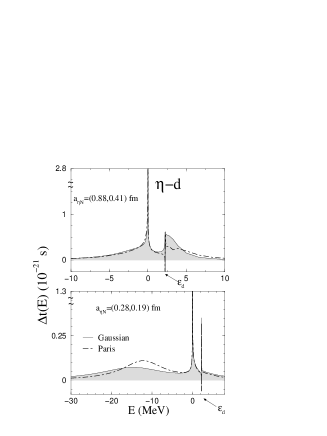
Figure 3: The delay time in $\eta$-deuteron elastic scattering as a function of the energy $E=\sqrt{s}-m_{\eta}-m_{d}$, where $\sqrt{s}$ is the total energy available in the $\eta d$ centre of mass system. The shaded curves are calculations using the Gaussian form of the deuteron wave function and dashed lines are evaluated using the Paris deuteron wave function. The vertical axis scale is broken in order to display the structure in the time delay plot clearly.

In Fig. 3, we plot the time delay in $\eta$ d $\rightarrow\eta$ d elastic scattering with two different inputs for the elementary $\eta N$ interaction. The $\eta N$ scattering lengths of $a_{\eta N}=(0.88,0.41)$ fm and $a_{\eta N}=(0.28,0.19)$ fm correspond to $\eta$d scattering lengths of $a_{\eta d}=(1.52,2.57)$ fm and $a_{\eta d}=(0.67,0.42)$ fm respectively. In both cases, we see a large positive time delay located near threshold. The solid lines (with shaded regions) are the calculations using a Gaussian form and the dashed lines with a Paris potential parametrization of the deuteron wave function. The vertical axis scale in Fig. 3 is broken in order to display the structure in the time delay plot clearly. We do not find a big difference in the results with the change of the wave function. In the case of the weaker $\eta N$ interaction, i.e. $a_{\eta N}=(0.28,0.19)$ fm, there appears a very broad bump around $-15$ MeV which could be due to an unstable bound state. On the positive energy side, there is a sharp negative time delay when the kinetic energy of the $\eta$-d system equals the binding energy of the deuteron. This behaviour is expected because of the connection of the energy derivative of the phase shift and hence the time delay (1) to the density of states as given by the Beth-Uhlenbeck formula [41]. It was shown in [15] that a maximum negative time delay occurs at the opening of an inelastic threshold. In the present case, the negative dip around $2.22$ MeV, corresponds to the break up threshold of the deuteron. We also see a resonance just near this inelastic threshold. However, the above result near the inelastic threshold should be taken with some caution since we have used the FRA which might not be a very good approximation at energies where new thresholds open up.

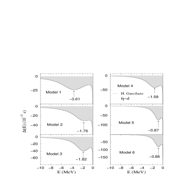
Figure 4: Quasivirtual states of the $\eta d$ system evaluated from a Faddeev calculation for $\eta d$ scattering. The various model numbers correspond to the different strengths of the $\eta N$ interaction as explained in [42].

Figure 5: Quasivirtual and quasibound states of the $\eta d$ system evaluated from a Faddeev calculation for $\eta d$ scattering using model 0 as mentioned in [42].

In order to check the validity of the above FRA approach for the $\eta d$ case (where it is known to have limitations [21]), we evaluate time delay using a model [42] which obtains the $\eta d$ elastic scattering amplitude using a relativistic version of the Faddeev equations described in [43]. The $\eta d$ amplitude in [42] is parametrized using the effective range formula:

$$f^{-1}_{\eta d}={1\over A_{\eta d}}\,+\,{1\over 2}\,R_{\eta d}\,k^{2}\,+\,S_{\eta d}\,k^{4}\,-i\,k$$ (19)

where $k$ is the momentum in the $\eta d$ centre of mass system and the parameters $A_{\eta d}$, $S_{\eta d}$ and $R_{\eta d}$ are as given in Table II of [42]. In Figs 4 and 5, we show the results obtained using the above amplitude. The time delay in Fig. 4 has been evaluated using $k\to-ik$ and hence the negative dips in this figure correspond to the quasivirtual states which appear as poles in the third quadrant of the complex k-plane. The locations of these dips (using different models as given in [42]) are exactly at the energy pole values given in Table III of [42] as expected. As explained already in Sec. II, such a negative time delay (or time advancement) is expected for quasivirtual states which give an exponential rise rather than an exponential decay law.

Figure 6: Magnitude of the complex amplitude $S=1+2ikf$ in the complex momentum plane evaluated from a Faddeev calculation for $\eta d$ scattering using model 0 as mentioned in [42]. The sharp pole corresponds to the quasibound state at $-16$ MeV as seen in the time delay plot in Fig. 5.

In the upper half of Fig. 5, we plot the time delay evaluated using $k\to-ik$ and the lower half shows the time delay plot corresponding to $k\to+ik$ in the amplitude with Model 0. Thus the negative dip in the upper half is the quasivirtual state as also given in Table II of [42] and the lower half shows the positive time delay corresponding to a quasibound or what we address as an “unstable bound” state in the present work. In order to demonstrate once again the one-to-one correspondence between the time delay peak and $S$-matrix poles, in Fig. 6 we plot the magnitude of $S$ as a function of the real and imaginary parts of momentum $k$. The pole occurs at ($-0.283+i0.674$) fm in the complex momentum plane. This corresponds to a peak value of about $-17$ MeV and a width of $35$ MeV which is in good agreement with the time delay plot in Fig. 5. Such a pole has however not been mentioned by the author in [42] (probably due to the fact that the author in [42] has been mostly concerned about the effect of the near threshold quasivirtual states on the $np\rightarrow d\eta$ reaction). We do not find any such positive peaks in any of the models shown in Fig. 4. It is interesting to note that as expected from [21], the FRA has some agreement with the Faddeev calculation for small $\eta N$ scattering lengths, $a_{\eta N}$, and the discrepancy increases for large $a_{\eta N}$.

Finally, we wish to caution the reader regarding the interpretation of time delay peaks in the case of $s$-wave scattering. To see this, substituting the phase shift expression, $S=exp(2i\delta)$ and comparing it with (17), one can write,

$$\delta={1\over 2i}\,{\rm ln}(1-{i\mu k\over\pi}t_{\eta A})\,=\,{1\over 2i}\,{\rm ln}(1+2ikf)$$ (20)

where $f$ is the scattering amplitude. For small $k$, $\delta\simeq kf$ and the behaviour of $d\delta/dE$ (the real part of which is essentially the time delay) is determined by the simple pole at $k=0$ (or $E_{\eta A}=E_{threshold}$) and the energy dependence of the scattering amplitude $f$. In the absence of a resonance, as $k\to 0$, $\delta=ka$, where $a=a_{R}+ia_{I}$ is the complex scattering length. For positive energies, $\Re e\delta=ka_{R}$, whereas for energies below zero, $k\to ik$ and $\Re e\delta=-ka_{I}$. In such a situation, $\Re e(d\delta/dE)$ exhibits a sharp peak at $E_{\eta A}=E_{threshold}$, the sign of which is determined by the sign of the scattering length. On the other hand, if the scattering amplitude has a resonant behaviour near threshold, one would see a superposition of the two behaviours. Consequently, a state reasonably close to threshold gets distorted in shape and one very close manifests simply by broadening the threshold singularity. A state far from threshold, however, remains completely unaffected.

5 The $\eta\,^{4}$He system

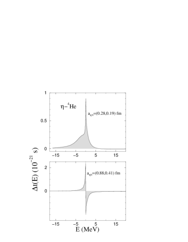
Figure 7: The delay time in $\eta\,^{4}$He elastic scattering as a function of the energy $E=\sqrt{s}-m_{\eta}-m_{\eta^{4}He}$, where $\sqrt{s}$ is the total energy available in the $\eta\,^{4}$He centre of mass system.

The time delay plot in the upper half of Fig. 7, shows once again the near threshold peak and one more broad one centered around $-2$ MeV. However, the plot with time delay evaluated using the model which gives $a_{\eta N}=(0.88,0.41)$ fm, shows a large negative time delay near threshold. The negative time delay can sometimes also arise due to a repulsive interaction [29]. Intuitively, an attractive interaction is something that causes resonance formation and “delays” the scattering process. A repulsive interaction on the other hand would speed up the process and the time taken for the process in the absence of interaction would be larger than that with interaction.

Before ending this section, we note that the $\eta^{4}$He scattering lengths obtained within the FRA and using two different models of the $\eta N$ interaction, namely, $a_{\eta N}=(0.88,0.41)$ fm and $a_{\eta N}=(0.28,0.19)$ fm are $a_{\eta\,^{4}He}=(-3.94,5.575)$ fm and $a_{\eta\,^{4}He}=(1.678,1.524)$ fm respectively.

6 Summary

In conclusion, we summarize the present work as:
(i) we have made a search for the unstable states of $\eta$-mesic deuteron and ⁴He extending the approach of time delay which was used recently for the first time in the eta-mesic case [9].
(ii) The established time delay method for searching resonances has been extended to negative energies, to search for bound, virtual and unstable bound states. The validity of this method has been established by applying it first to the known case of the $np$ system and then to the case of the $\eta$-d system within a parameterized Faddeev calculation.
(iii) The calculations were performed with different values of the $\eta N$ scattering length considered as acceptable in literature. Within the Faddeev equation parameterization, we find one unstable bound state far from threshold ($\sim-16$ MeV) for an $\eta N$ scattering length of $(0.42,0.34)$ fm. Within the FRA calculation, we find such an $\eta d$ state around $-12$ MeV for $a_{\eta N}=(0.28,0.19)$ fm. These results seem to indicate that though the FRA in general is not recommendable for $\eta d$ elastic scattering, the results are close to those from the Faddeev calculations for low values of the $\eta N$ scattering length.
(iv) In the $\eta^{4}$He case, within the FRA calculations, we find an unstable bound state close to threshold for a small scattering length of $(0.28,0.19)$ fm.

References

- [1] Q. Haider, L. Liu, Phys. Lett. B 172, 257 (1986); ibid 174, 465(E) (1986).
- [2] R. S. Bhalerao, L. C. Liu, Phys. Rev. Lett. 54, 865 (1985).
- [3] M. Pfeiffer et al., Phys. Rev. Lett. 92, 252001 (2004).
- [4] G. A. Sokol et al., Part. Nucl. Lett. 102, 71 (2000); G. A. Sokol and L. N. Pavlyuchenko, arXiv:nucl-ex/0111020.
- [5] N. Willis et al., Phys. Lett. B 406, 14 (1997); arXiv:nucl-ex/9703002
- [6] B. Mayer et al., Phys. Rev. C 53, 2068 (1996); J. Berger et al., Phys. Rev. Lett. 61, 919 (1988).
- [7] H. Calen et al., Phys. Rev. Lett. 80, 2069 (1998); H. Calen et al., Phys. Rev. Lett. 79, 2642 (1997).
- [8] M. Ulicny [GEM Collaboration], “Measurement of the reaction near threshold energies”, AIP Conf. Proc. 603, 543 (2001).
- [9] N. G. Kelkar, K. P. Khemchandani and B. K. Jain, J. Phys. G:Nucl. Part. Phys. 32, L19 (2006); arXiv:nucl-th/0601080.
- [10] L. Eisenbud, dissertation, Princeton, June 1948 (unpublished).
- [11] E. P Wigner, Phys. Rev. 98, 145 (1955); E. P. Wigner and L. Eisenbud Phys. Rev. 72, 29 (1947).
- [12] C. J. Joachain 1975 Quantum Collision Theory (North-Holland); J. R. Taylor 1972 Scattering Theory: The Quantum theory on non-relativistic collisions (John Wiley and Sons, Inc.); M. L. Goldberger and Watson 1964 Collision Theory (New York; John Wiley); Arno Böhm 1979 Quantum Mechanics (Springer-Verlag); A. Messiah 1961 Quantum Mechanics (V. I. North-Holland Publishing Company, Amsterdam).
- [13] N. G. Kelkar, M. Nowakowski, K. P. Khemchandani, J. Phys. G: Nucl. Part. Phys. 29, 1001 (2003), hep-ph/0307134; ibid, Mod. Phys. Lett. A 19, 2001 (2004), nucl-th/0405008; N. G. Kelkar and M. Nowakowski, hep-ph/0412240, Talk given at International Workshop on PENTAQUARK04, Spring-8, Hyogo, Japan, 20-23 Jul 2004 (to appear in the proceedings).
- [14] N. G. Kelkar, M. Nowakowski and K. P. Khemchandani, Nucl. Phys. A724, 357 (2003), hep-ph/0307184; M. Nowakowski and N. G. Kelkar, hep-ph/0411317, Talk given at International Workshop on PENTAQUARK04, Spring-8, Hyogo, Japan, 20-23 Jul 2004 (to appear in the proceedings).
- [15] N. G. Kelkar, J. Phys. G: Nucl. Part. Phys. 29, L1 (2003), hep-ph/0205188.
- [16] N. G. Kelkar, M. Nowakowski, K. P. Khemchandani and S. R. Jain, Nucl. Phys. A730, 121 (2004), hep-ph/0208197.
- [17] K. P. Khemchandani, N. G. Kelkar, B. K. Jain, Nucl. Phys. A708, 312 (2002), nucl-th/0112065.
- [18] Q. Haider and L. C. Liu, Phys. Rev. C 66, 045208 (2002).
- [19] T. Ueda, Phys. Rev. Lett. 66, 297 (1991).
- [20] S. A. Rakityansky, S. A. Sofianos, N. V. Shevchenko, V. B. Belyaev, W. Sandhas, Nucl. Phys. A684, 383 (2001); N. V. Shevchenko, V. B. Belyaev, S. A. Rakityansky, S. A. Sofianos, W. Sandhas, Eur. Phys. J. A 9, 143 (2000), arXiv:nucl-th/9908035.
- [21] N. V. Shevchenko, S. A. Rakityansky, S. A. Sofianos, V. B. Belyaev, W. Sandhas, Phys. Rev. C 58, R3055 (1998), arXiv:nucl-th/9808009.
- [22] H. Garcilazo and M. T. Peña, Phys. Rev. C 63, 021001 (2001).
- [23] A. Deloff, Phys. Rev. C 61, 024004 (2000).
- [24] A. Fix and H. Arenhövel, Eur. Phys. J A 9, 119 (2000); ibid, Nucl. Phys. A697, 277 (2002).
- [25] S. A. Rakityansky, S. A. Sofianos, M. Braun, V. B. Belyaev and W. Sandhas, Phys. Rev. C 53 (1996) R2043; S. A. Rakityansky, S. A. Sofianos, V. B. Belyaev, W. Sandhas, Few-Body Systems Suppl., 9, 227 (1995).
- [26] A. Fix and H. Arenhövel, MKPH-T-02-03, Jun 2002; “Interaction of eta mesons with a three-nucleon system”, arXiv:nucl-th/0206038, Published in Cracow (2002) “Production, properties and interaction of mesons”, 383-387.
- [27] S. Wycech and A. M. Green, Phys. Rev. C 64, 045206 (2001); arXiv:nucl-th/0104053.
- [28] G. Calucci, L. Fonda, G. C. Ghirardi, Phys. Rev. 166, 1719 (1968); H. C. Ohanian, C. G. Ginsburg, Am. Journal of Phys. 42, 310 (1974); A. I. Baz, JETP 33 (1957) 923; H. M. Nussenzveig, Phys. Rev. D 6, 1534 (1972); H. M. Nussenzveig, Phys. Rev. A 55, 1012 (1997).
- [29] F. T. Smith, Phys. Rev. 118, 349 (1960).
- [30] B. H. Bransden and R. Gordon Moorhouse 1973 The Pion-Nucleon System (Princeton University Press, New Jersey).
- [31] Asher Peres, Annals of Physics 37, 179 (1966).
- [32] O. Morimatsu and K. Yazaki, Nucl. Phys. A435, 727 (1985).
- [33] J. Fraxedas and J. Sesma, Phys. Rev. C 37, 2016 (1988).
- [34] M. Lacombe et al., Phys. Lett. B101 (1981) 139.
- [35] L. I. Schiff 1949 Quantum Mechanics, (McGraw-Hill Book Company, Inc., New York).
- [36] V. B. Belyaev, Lectures on the theory of FEW BODY SYSTEMS, Springer series in Nuclear and Particle Physics, 1990.
- [37] S. A. Rakityansky and S. A. Sofianos, Proceedings of The European Conference on Advances in nuclear physics and related areas, Thessaloniki-Greece, (1997) 570, Giahoudi-Giapouli Publishing, Thessaloniki, 1999.
- [38] A. M. Green, S. Wycech, Phys. Rev. C 60, 035208 (1999); ibid Phys. Rev. C 55, 2167 (1997).
- [39] M. Batinić, I. Dadić,I. Šlaus, A. Švarc, B. M. K. Nefkens and T. S. H. Lee, Physica Scripta 58, 15 (1998); nucl-th/9703023 (1997); M. Batinić, I. Šlaus, A. Švarc, Phys. Rev. C 52, 2188 (1995); ibid B. M. K. Nefkens, Phys. Rev. C 51, 2310 (1995), Erratum - C 57, 1004 (1998).
- [40] A. M. Green and S. Wycech, Phys. Rev. C 71, 014001 (2005).
- [41] E. Beth and G. E. Uhlenbeck, Physics 4, 915 (1937); K. Huang, Statistical Mechanics (Wiley, New York, 1963).
- [42] H. Garcilazo, Phys. Rev. C 71, 048201 (2005).
- [43] H. Garcilazo, Phys. Rev. C 67, 055203 (2003).