TRI-PP-06-08

A Wilsonian renormalization group (WRG) equation for nuclear current operators in two-nucleon systems is derived. Nuclear current operators relevant to low-energy Gamow-Teller transitions are analyzed using the WRG equation. We employ the axial two-body current operators from phenomenological models and heavy-baryon chiral perturbation theory, which are quite different from one another in describing small scale physics. After reducing the model space of the operators using the WRG equation, we find that there still remains a significant model dependence at $\Lambda=200$ MeV, where $\Lambda$ is the sharp cutoff specifying the size of the model space. A model independent effective current operator is found at a rather small cutoff value, $\Lambda=70$ MeV. By simulating the effective current operator at $\Lambda=70$ MeV, we obtain a current operator based on a pionless theory, thereby arguing that an equivalence relation exists between nuclear current operators of phenomenological models and those of effective field theories.

PACS(s): 05.10.Cc, 25.10.+s.

1. Introduction

A theoretical framework, based on the idea of effective field theory, for describing nuclear system was proposed at the beginning of 1990’s by Weinberg [1]. The framework provides us with a systematic scheme for constructing nuclear operators such as nuclear forces and nuclear electroweak currents from an effective Lagrangian of the underlying theory. We will refer to it as nuclear effective field theory (NEFT). For reviews, see, e.g., Refs. [2, 3, 4, 5, 6] and references therein. Meanwhile, phenomenological models for the nuclear operators have been conventionally used in nuclear physics. Expressions and behaviors of those nuclear operators are quite different among the phenomenological models and NEFT, whereas all of the nuclear operators give essentially the same reaction rates for low-energy reactions in few-nucleon system, e.g., solar-neutrino reactions on the deuteron[7, 8, 9, 10]. This implies that there exists an equivalence relation between the nuclear operators of phenomenological models and NEFT, and thus it is interesting to seek for the relation.

Recently, one of the authors (SXN) argued the relation for the nuclear forces from a viewpoint of the renormalization group (RG) [11]. In that work, the author formulated a “scenario”, which we describe in detail in the followings, for the relation between the nuclear forces based on NEFT ($V_{EFT}$) and phenomenological nuclear forces ($V_{ph}$) paying attention to a difference in the size of the model space between $V_{EFT}$ and $V_{ph}$. One may construct many different $V_{ph}$ all of which reproduce the low-energy $NN$-data. Those nuclear forces are different from one another in modeling small scale phenomena. As high-momentum states of the nucleon are integrated out and thus the model space of $V_{ph}$ is reduced, information relevant to the details of the small scale physics are gradually lost. As a result, all $V_{ph}$ eventually converge to a single nuclear force defined in a sufficiently small model space; the model dependence found in the original $V_{ph}$ disappears. The short-range part of the single low-momentum interaction is accurately parameterized with the use of simple contact interactions, which is the way NEFT describes the small scale physics. After all, the parameterization of the single low-momentum interaction is nothing more than $V_{EFT}$. By construction, $V_{EFT}$ obtained in this way does not have a dependence on modeling the small scale physics. This is the scenario for the relation among $V_{EFT}$ and $V_{ph}$. In Ref. [11], the author employed a Wilsonian renormalization group (WRG) equation derived by Birse, McGovern and Richardson [13] for the model space reduction, and showed a result to convincingly argue that the scenario for the relation between $V_{ph}$ and $V_{EFT}$ is realized.

It would be interesting to extend the WRG analysis to the study of nuclear electroweak currents. This is the main subject of this paper. Similar to the nuclear forces, the expression and behavior of a nuclear exchange current operator of a phenomenological model are quite different from those of another model or NEFT, and thus the reaction mechanism of an electroweak process is also model dependent. The model dependence stems from modeling small scale physics. Thus, if one reduces the model spaces of the different nuclear current operators, it is expected that all the operators evolve to be essentially a single nuclear current, which may be accurately simulated by the NEFT-based parameterization. In this way, nuclear electroweak currents from phenomenological models and from NEFT are related through RG.

In this work, we derive a WRG equation of nuclear current operator for two-nucleon system. By using the WRG equation, we reduce the model space of nuclear current operators of either phenomenological models or NEFT with the pion, and examine the evolution of the operators. We are specifically concerned with the axial vector current associated with the Gamow-Teller transition in the low-energy neutral-current neutrino reaction on the deuteron ($\nu d\rightarrow\nu pn$), where our analysis can be simplified due to the absence of the Coulomb interaction. Finally, the effective operator, obtained as a result of the model-space reduction, is simulated by a NEFT-based operator without the pion [15].

Here, we mention a choice of the model-space reduction scheme. So far, some methods have been used to derive a low-momentum $NN$ interaction from phenomenological $NN$ interactions. Those methods are the WRG method[11, 13], the Lee-Suzuki method[12, 16], and the unitary transformation method[17]. For detailed comparison of them, see Ref. [18]. In Ref. [11], the author argued that the use of the WRG method is consistent with the construction of the effective Lagrangian in NEFT. This argument is based on that an effective Lagrangian in NEFT is in principle obtained by integrating out high-energy degrees of freedom within the path integral formalism, and that solving the WRG equation is equivalent to performing a path integral. Also in the reference, the three model-space reduction schemes are applied to the nuclear forces and it is shown that only the WRG method generates an effective low-momentum interaction which is accurately simulated by the NEFT-based parameterization of the nuclear forces, even in a case of a small model space relevant to a pionless EFT [EFT( / $\pi$ )]. Therefore, we regard the WRG method as being the most appropriate for studying the relation between the models and NEFT, and we adopt it as the model-space reduction method in this work.

This paper is organized as follows. In Sec. 2, we derive the WRG equation of the nuclear current operators for two-nucleon system. In Sec. 3, we present the current operators employed in this work, and give a detailed description of our numerical analysis. In Sec. 4, we show results of the numerical calculation and give discussion on our results. Finally, we give a concluding remark in Sec. 5. In appendices, we give a detailed derivation of the WRG equation, a discussion of a conservation law for an effective current operator, and a discussion on a role of the tensor nuclear force in a pionless theory.

2 Wilsonian renormalization group equation for nuclear current operator

We briefly discuss a Wilsonian renormalization group (WRG) equation for nuclear current operators. A detailed derivation of the WRG equation is given in Appendix A. We start with a matrix element of a current operator in a two-nucleon system evaluated in the momentum space,

$$\langle O\rangle=\int_{0}^{\Lambda}\!\!\!k^{2}dk\int_{0}^{\Lambda}\!\!\!k^{\prime 2}dk^{\prime}\;\psi_{p^{\prime}}^{(\beta)*}(k^{\prime})\;O^{(\beta,\alpha)}(k^{\prime},k)\;\psi_{p}^{(\alpha)}(k)\ ,$$ (1)

where $\psi_{p}^{(\alpha)}(k)$ ($\psi_{p^{\prime}}^{(\beta)}(k^{\prime})$) is the radial part of the wave function for the initial (final) two-nucleon state, which are derived from an effective interaction with a cutoff $\Lambda$ (see Eq. (14) in Appendix A). The quantity $p$ ($p^{\prime}$) is an on-shell relative momentum for the initial (final) two-nucleon state, $p\equiv\sqrt{ME}$ ($p^{\prime}\equiv\sqrt{ME^{\prime}}$) with $E$ ($E^{\prime}$) being the energy for the relative motion of the two nucleons and $M$ is the nucleon mass, and $\alpha$ ($\beta$) specifies a partial wave. The radial part of the current operator between the $\beta$ and $\alpha$ partial waves are denoted by $O^{(\beta,\alpha)}(k^{\prime},k)$. The quantities $k$ and $k^{\prime}$ are the magnitudes of the relative off-shell momenta of the two-nucleon system. The cutoff $\Lambda$, which is the maximum magnitude of the relative momenta, specifies the size of the model space spanned by plane wave states of the two-nucleon system.

We differentiate the both sides of Eq. (1) and impose a condition that the matrix element is invariant with respect to changes in $\Lambda$, i.e., $d\langle O\rangle/d\Lambda=0$. This leads to the WRG equation for the effective current operator,

$${\partial O^{(\beta,\alpha)}_{\Lambda}(k^{\prime},k;p^{\prime},p)\over\partial\Lambda}$$

$$={M\over 2\pi^{2}}\left({O^{(\beta,\alpha)}_{\Lambda}(k^{\prime},\Lambda;p^{\prime},p)V^{(\alpha)}_{\Lambda}(\Lambda,k;p)\over 1-p^{2}/\Lambda^{2}}\right.+\left.{V^{(\beta)}_{\Lambda}(k^{\prime},\Lambda;p^{\prime})O^{(\beta,\alpha)}_{\Lambda}(\Lambda,k;p^{\prime},p)\over 1-p^{\prime 2}/\Lambda^{2}}\right)\ ,$$ (2)

where $V^{(\alpha)}_{\Lambda}(k^{\prime},k;p)$ is an effective $NN$-potential for a partial wave $\alpha$, which evolves following the WRG equation for a $NN$ potential [11, 13]. In $V^{(\alpha)}_{\Lambda}(k^{\prime},k;p)$, $k$ ($k^{\prime}$) denotes the off-shell relative momentum of the two nucleons before (after) the interaction, $p$ denotes the on-shell momentum, and $\Lambda$ is the cutoff value specifying the model space. Some arguments in the current operator, which have been suppressed in Eq. (1) for simplicity, are shown. We note that, because the current operator and $NN$ potential are evolved by means of the WRG equation, the effective current operator acquires a dependence on both the initial and final on-shell momenta, $p$ and $p^{\prime}$ ($E$ and $E^{\prime}$), whereas the effective $NN$-potential acquires a dependence on either the on-shell momentum of the initial state or that of the final state, $p$ or $p^{\prime}$ ($E$ or $E^{\prime}$). A graphical representation of Eq. (S0.Ex1) is shown in Fig. 1.

Figure 1: A graphical representation of the WRG equation for a current operator. $O$ ($O^{\prime}$) is an original (renormalized) current operator and $V$ is a $NN$-interaction. In the loops, the magnitude of the relative momentum of the two nucleons is denoted by $\bar{k}$, which lies in the momentum shell that is integrated out.

For an infinitesimal reduction of the cutoff, the operator $O$ evolves into the renormalized one $O^{\prime}$ by absorbing the one-loop graph either before or after the insertion of the current operator. The loops include the intermediate two-nucleon states of $\Lambda-\delta\Lambda\leq\bar{k}\leq\Lambda$, where $\bar{k}$ is the magnitude of the relative momentum. The WRG equation given by Eq. (S0.Ex1) is for a single $NN$ partial wave, but an extension to a coupled-channel case is straightforward.

One starts with $O=O_{\bar{\Lambda}}$ for a cutoff $\bar{\Lambda}$ and derives $O_{\Lambda}$ for $\Lambda(<\bar{\Lambda})$ by solving the WRG equation. A solution (integral form) of the WRG equation, Eq. (S0.Ex1), may be written as

$$O_{\Lambda}^{(\beta,\alpha)} = \eta\left(O_{\bar{\Lambda}}^{(\beta,\alpha)}+O_{\bar{\Lambda}}^{(\beta,\alpha)}\lambda{1\over E-H_{\bar{\Lambda}}^{(\alpha)}}\lambda V_{\bar{\Lambda}}^{(\alpha)}+V_{\bar{\Lambda}}^{(\beta)}\lambda{1\over E^{\prime}-H_{\bar{\Lambda}}^{(\beta)}}\lambda O_{\bar{\Lambda}}^{(\beta,\alpha)}\right.$$ (3)

$$+ \left.V_{\bar{\Lambda}}^{(\beta)}\lambda{1\over E^{\prime}-H_{\bar{\Lambda}}^{(\beta)}}\lambda O_{\bar{\Lambda}}^{(\beta,\alpha)}\lambda{1\over E-H_{\bar{\Lambda}}^{(\alpha)}}\lambda V_{\bar{\Lambda}}^{(\alpha)}\right)\eta\ ,$$

where $H_{\bar{\Lambda}}^{(\alpha)}$, $V_{\bar{\Lambda}}^{(\alpha)}$ are the full Hamiltonian and the $NN$-interaction for a partial wave $\alpha$, respectively, defined in the model space with $\bar{\Lambda}$. Furthermore, $\eta$ and $\lambda$ are the projection operators defined by

$$\eta = \int{\bar{k}^{2}d\bar{k}\over 2\pi^{2}}\left|\bar{k}\,\right\rangle\left\langle\bar{k}\,\right|\,\,,\quad\quad\quad\bar{k}\leq\Lambda\,\,,$$ (4)

$$\lambda = \int{\bar{k}^{2}d\bar{k}\over 2\pi^{2}}\left|\bar{k}\,\right\rangle\left\langle\bar{k}\,\right|\,\,,\quad\quad\quad\Lambda<\bar{k}\leq\bar{\Lambda}\,\,,$$ (5)

where $|\bar{k}\rangle$ represents the radial part of the free two-nucleon states with the relative momentum $\bar{k}$. By inserting Eq. (3) into Eq. (S0.Ex1), one can easily check that the integral form of the WRG equation, Eq. (3), satisfies its differential form, Eq. (S0.Ex1).

A nuclear current operator has the properties which a nuclear force does not possess, i.e., the current operator satisfies a (partial) conservation law. It is interesting to examine the conservation law for the effective current operator obtained after the model-space reduction. This subject is discussed in Appendix B.

3. Nuclear current operators

In this section, we introduce the nuclear current operators used in our numerical renormalization group analysis. We employ five nuclear current operators contributing to the GT transition: two of them are phenomenological models and the others are based on pionful EFT [EFT($\pi$)] with three cutoff values . Each of the five operators has the same one-body operator,

$$\vec{A}_{1}(\vec{x}) = -g_{A}\sum_{i}{\tau^{3}_{i}\over 2}\,\vec{\sigma}_{i}\,\delta^{(3)}(\vec{x}-\vec{r}_{i})\ ,$$ (6)

where $g_{A}$ is the axial-vector coupling constant, and $\vec{\tau}_{i}$ and $\vec{\sigma}_{i}$ are the isospin and spin operators, respectively, for the $i$-th nucleon. The isospin operator has only the third component, $\tau^{3}_{i}/2$, because we consider the neutral-current reaction, $\nu d\to\nu pn$, in this work. It is noted that we neglect the small corrections from the axial form factor, the induced pseudoscalar current, and corrections from higher order terms (e.g., $1/M$ corrections) because we are concerned with the reaction in a low-energy region, $E_{\nu}<20$ MeV, where $E_{\nu}$ is the incoming neutrino energy.

Figure 2: Diagrams for axial-vector exchange currents of phenomenological models. Upper two diagrams (a,b) are for the $\Delta$-excitation currents induced by the $\pi$ (or $\rho$) exchange. Lower diagrams (c) and (d) are for the $\pi$ (or $\rho$) exchange pair currents, and diagram (e) is for the $\pi$-$\rho$ current.

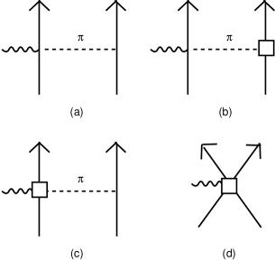
Figure 3: Diagrams for axial-vector exchange currents from EFT($\pi$). Dashed lines denote pions and vertices without (with) white box arise from the leading (sub-leading) order Lagrangian.

We now present the two-body operators. The operators of two phenomenological models are found, e.g., in Ref. [8]. The operator for one of the models are obtained by calculating five diagrams shown in Fig. 3. The model was originally proposed in Ref. [20] and the strength of the $\Delta$-excitation currents in the model was fixed to reproduce the experimental tritium $\beta$-decay rate. We will refer to the model as “Model I”. The other model consists of only the $\Delta$-excitation currents (the upper two diagrams in Fig. 3). The overall strength of the model was adjusted so as to reproduce the same total cross section for $\nu d\rightarrow\nu pn$ as that of Model I at the reaction threshold. We will refer to this model as “Model II”. For explicit expressions of the operators, see Eqs. (22)-(26) of Ref. [8].

The nuclear currents based on EFT($\pi$) are obtained from heavy-baryon chiral Lagrangian up to next-to-next-to-next-to leading order in Refs. [10, 21]. Diagrams for the two-body current operator are shown in Fig. 3 and explicit expressions for the operators are given in, e.g., Eq. (20) in Ref. [21]. We use three EFT($\pi$)-based operators with different cutoff values, $\Lambda_{eft}=500$, 600, and 800 MeV (see the footnote 8). For each of the cutoff values, the coupling constant of the axial-vector-four-nucleon contact interaction shown by diagram (d) in Fig. 3 has been fixed so as to reproduce the tritium $\beta$-decay rate [22].

In our numerical analysis, we consider the operator, $O$, obtained with the current operators, $A(\vec{x})$, presented above,

$$O=\int d\vec{x}\ e^{i\vec{q}\cdot\vec{x}}{\cal A}(\vec{x})\ ,$$ (7)

where ${\cal A}(\vec{x})\equiv A(\vec{x})|_{\vec{R}=0}$, with $A(\vec{x})$ being the axial-vector current. The center of mass coordinate of the two nucleons is denoted by $\vec{R}$. The quantity $\vec{q}$ is the momentum transfer to the nuclear current operator. We will examine the evolution of the operator $O$ defined in Eq. (7), rather than the current operator $A(\vec{x})$ itself, using the WRG equation. Also, a matrix element we calculate is always that of the operator $O$. In what follows, we refer to the operator $O$ in Eq. (7) also as “current operator”.

Matrix elements of the operators are calculated before a model-space reduction ($\Lambda=\infty$), and the numerical results are shown in Table 1. We calculate contributions (ratio) to the matrix elements from the one-body and the two-body current operators. We decompose the contributions from the two-body operators into those from the deuteron $S$ and $D$-wave states. For the final neutron-proton scattering state, we consider only the ${}^{1}S_{0}$ partial wave, which is the dominant state in the low-energy region. The total amplitude from “Model I” is normalized to 100%. In calculating the matrix elements, we employ a specific kinematic condition: $E=-B$, $E^{\prime}=1$ MeV, and $q=30$ MeV where $B$ is the deuteron binding energy and $q=|\vec{q}|$. The wave functions are obtained with the Argonne v18 potential[24]. Since all of the five operators have the same one-body operator, we have the same contribution from the one-body operator with the deuteron $S$- and $D$-waves, 98.87%. Meanwhile, the five two-body currents give small contributions which agree with each other within 1% accuracy. We have 1.13, 0.72, 1.42, 1.41, 1.40% contributions from the two-body currents with the deuteron $S$- and $D$-waves from the Model I and II, and EFT($\pi$) with the three cutoff values $\Lambda_{eft}=500$, 600, and 800 MeV, respectively.

$\Lambda$	Model	$\langle\mbox{1B}\rangle$	$\langle\mbox{2B}\rangle$	$\langle\mbox{2B}\rangle$
(MeV)		$S+D$ (%)	$S+D$ (%)	$S$ (%)	$D$ (%)
	Model I	98.87	1.13	-0.33	1.46
	Model II	98.87	0.72	0.00	0.72
$\infty$	$\Lambda_{eft}=500$ MeV	98.87	1.42	-1.18	2.60
	$\Lambda_{eft}=600$ MeV	98.87	1.41	-2.00	3.41
	$\Lambda_{eft}=800$ MeV	98.87	1.40	-3.26	4.65
	Model I	97.05	2.96	2.85	0.12
	Model II	97.05	2.56	2.50	0.06
200	$\Lambda_{eft}=500$ MeV	97.05	3.25	3.05	0.20
	$\Lambda_{eft}=600$ MeV	97.05	3.25	3.04	0.21
	$\Lambda_{eft}=800$ MeV	97.05	3.23	3.01	0.22
	Model I	69.22	30.79	30.77	0.03
	Model II	69.22	30.39	30.36	0.03
70	$\Lambda_{eft}=500$ MeV	69.22	31.08	31.05	0.03
	$\Lambda_{eft}=600$ MeV	69.22	31.08	31.05	0.03
	$\Lambda_{eft}=800$ MeV	69.22	31.06	31.04	0.03

Table 1: Contributions (ratio) to the Gamow-Teller (GT) matrix element, $\langle^{1}S_{0}|O|^{3}S_{1}(^{3}D_{1})\rangle$, from each component of the current operators. The model space reduction using the WRG equation introduces the sharp cutoff and the values of it are shown in the first column. Each current operator is obtained from Model I and II, and EFT($\pi$) with $\Lambda_{eft}=500$, 600, 800 MeV, shown in the second column. The third and fourth columns give the contribution from the one-body (1B) and the two-body (2B) operators, respectively. The 2B contributions are from the deuteron ${}^{3}S_{1}$ and ${}^{3}D_{1}$ waves, which are separately given in the fifth and sixth columns (denoted by $S$ and $D$). For more details, see the text.

We can see from the table that the behaviors of the two-body currents are quite different. Model I and II induce the ${}^{3}D_{1}\to{}^{1}S_{0}$ transitions (1.47 and 0.72%) more strongly than the ${}^{3}S_{1}\to{}^{1}S_{0}$ ones ($-0.33$ and 0.00%), because the important operator in the models is the tensor-type originated from the $\Delta$-excitation currents exchanging a pion or a rho meson. In contrast, the EFT($\pi$)-operators generate the ${}^{3}S_{1}\to{}^{1}S_{0}$ transition amplitudes ($-1.18$, $-2.00$, and $-3.26$% for $\Lambda_{eft}=500$, 600, and 800 MeV, respectively) and ${}^{3}D_{1}\to{}^{1}S_{0}$ ones ($2.60$, $3.41$, and $4.65$%), both of which are larger than those of Model I and II. The ${}^{3}S_{1}\to{}^{1}S_{0}$ transition is due to the contact interaction, the diagram (d) in Fig. 3, whereas the ${}^{3}D_{1}\to{}^{1}S_{0}$ transition is due to the pion exchange two-body currents, mainly the diagram (c) in Fig. 3. We find that a larger cutoff value ($\Lambda_{eft}$) leads to a more destructive interference between the deuteron $S$ and $D$-wave contributions. The interference between the two transitions are so destructive for the EFT($\pi$)-based operators and thus the net contribution is almost the same as those of Model I and II.

4. WRG analysis of the current operators

Starting with the five sets of the nuclear operators discussed in the previous section, we calculate effective operators at the cutoff values $\Lambda=200$ and 70 MeV using the integral form of the WRG equation, Eq. (3). In this work, we define the one- and two-body effective currents as

$$O^{eff}_{1} = \eta O_{1}\eta\,,$$ (8)

$${O}^{eff}_{2} = \eta\left[O_{2}+(O_{1}+O_{2})\lambda\frac{1}{E-H}\lambda V+V\lambda\frac{1}{E^{\prime}-H}\lambda(O_{1}+O_{2})\right.$$ (9)

$$\left.+V\lambda\frac{1}{E^{\prime}-H}\lambda(O_{1}+O_{2})\frac{1}{E-H}\lambda V\right]\eta\,,$$

where $O_{1}$ and $O_{2}$ are the “bare” one- and two-body current operators, respectively, which we have already introduced. We note that the high energy parts of the bare one-body current operator $O_{1}$ are included in $O_{2}^{eff}$, as graphically shown in Fig. 4. The cutoffs in the projection operators, $\eta$ and $\lambda$ in Eqs. (4) and (5), are thus $\bar{\Lambda}=\infty$ and $\Lambda=200$ or 70 MeV.

In our WRG analysis, we observe that the effective two-body operators suddenly jump up at a momentum around the cutoff. (We will see it below.) As shown in Eq. (9) (graphically in Fig. 4), the bare one-body current operator can give a contribution to the effective two-body operator, and this is the origin of the “jump-up” structure in the effective operators.

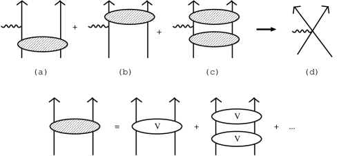
Figure 4: A graphical representation of the renormalization of the effective two-body operator due to the one-body operator. In the diagrams (a)-(c), all external two-nucleon systems have the relative momentum belonging to the model space while all the intermediate states are the high momentum states to be integrated out. After the model-space reduction, the diagrams (a)-(c) contribute to the renormalization of the two-body operator shown by the diagram (d).

In Fig. 4(a) (Fig. 4(b)), the high momentum states before (after) the insertion of the current operator are integrated out whereas, in Fig. 4(c), the high momentum states before and after the insertion of the current are integrated out to renormalize the two-body operator. The diagrams (a), (b) and (c) in Fig. 4 correspond to the $O_{1}$ part of the second, third and fourth terms in Eq. (9), respectively. Because of the momentum conservation, these terms of Figs. 4(a)-(c) give non-vanishing contributions only if the condition, $\left|\bar{k}-{q\over 2}\right|\leq\bar{k}^{\prime}\leq\bar{k}+{q\over 2}$, is satisfied; $\bar{k}$ ($\bar{k}^{\prime}$) is the magnitude of the relative momentum of the two-nucleon state just before (after) the insertion of the current operator. The diagrams, Figs. 4(a) and (b), start generating a large amount of the contributions at a certain kinematical point. For example, the $O_{1}$ part of the second term in Eq. (9) gives non-vanishing contribution for

$$\left|\Lambda-{q\over 2}\right|\leq k^{\prime}\leq\Lambda\ .$$ (10)

The behavior of the renormalized effective two-body operators thus changes suddenly at the value of the momentum $k$ ($k^{\prime}$), as discussed above.

4.1 Effective current operators at $\Lambda=200$ MeV

Now we are in a position to discuss our result of the effective operators for $\Lambda=200$ MeV. We reduce the model space of Model I or II or EFT($\pi$) using the WRG equation, and evaluate the GT matrix elements for the kinematics specified before. The result is shown in Table 1. The contribution from the effective one-body operator, 97.05%, is smaller than that (98.87%) for $\Lambda=\infty$ by 1.82%. This is because a part of the one-body operator sensitive to the high momentum part of the wave functions is renormalized into the effective two-body operator. In addition, we find that most of the two-body $D$-wave contributions at $\Lambda=\infty$ are also renormalized into the two-body $S$-wave ones at $\Lambda=200$ MeV. We can see that there still remains some model dependence among the models and EFT($\pi$) at $\Lambda=200$ MeV. On the other hand, the three EFT($\pi$)-based operators, which appear differently at $\Lambda=\infty$, give almost the same result at $\Lambda=200$ MeV.

In Figs. 6 and 6, we show the radial part of effective two-body current operators for $\Lambda=200$ MeV obtained from the EFT($\pi$)-based operators. We denote the effective operator for the initial deuteron $S$- and $D$-wave states (and the final ${}^{1}S_{0}$ state) by $O_{2,SS}^{eff}(k^{\prime},k)$ and $O_{2,SD}^{eff}(k^{\prime},k)$, respectively. We plot the diagonal part of them, i.e., $k^{\prime}=k$, and also that of the “bare” current operators, $O_{2,SS}(k,k)$ and $O_{2,SD}(k,k)$.

Figure 5: Effective two-body operators ($\Lambda=200$ MeV), $O_{2,SS}^{eff}$, for the deuteron $S$-wave state from EFT($\pi$)-based $O_{2,SS}$. The diagonal momentum-space matrix elements are shown. The lower three dotted curves represent the original $O_{2,SS}$; from the bottom, $\Lambda_{eft}=800,600$ and 500 MeV. The upper three curves represent the $O_{2,SS}^{eff}$. The solid, dashed and dash-dotted curves are the effective two-body currents obtained from EFT($\pi$) with $\Lambda_{eft}=500,600$ and 800 MeV, respectively.

Figure 6: Effective two-body operators ($\Lambda=200$ MeV), $O_{2,SD}^{eff}$, for the deuteron $D$-wave state from EFT($\pi$)-based $O_{2,SD}$. Three dotted curves represent the original $O_{2,SD}$, from the bottom, for $\Lambda_{eft}=500,600$ and 800 MeV. The other three curves represent the $O_{2,SD}^{eff}$. The solid, dashed and dash-dotted curves are for $\Lambda_{eft}=500,600$ and 800 MeV, respectively. Scale of vertical axis is ten times as small as that of Fig. 6. The other features are the same as those in Fig. 6.

We find that the curves of the effective operators in the figures suddenly change at $k=\Lambda-q/2=185$ MeV (“jump-up” structure). This is because, as discussed above, at this point the diagrams Figs 4(a) and (b) start contributing to the effective two-body operators. We also find that the cutoff $\Lambda_{eft}$ dependence among the original EFT($\pi$)-based operators at $\Lambda=\infty$ are much less observed at this resolution of the system. However, the disappearance of the model dependence is not as perfect as the case for the nuclear force, $V_{low\mbox{-}k}$, in which the model dependence of phenomenological nuclear forces are almost not observed at $\Lambda(=2.1\mbox{\rm fm}^{-1})\simeq 400$ MeV[11, 12]. We find that there still remains a significant model dependence ($\Lambda_{eft}$-dependence) for $\Lambda\simeq$ 400 MeV (we did not show it), and that the model dependence of the central-type EFT($\pi$)-based nuclear current almost disappears at $\Lambda=200$ MeV (Fig. 6). Furthermore, we observe the model dependence in the tensor-type operator even at $\Lambda=200$ MeV (Fig. 6). This result has been expected because all of the operators have the same pion-range mechanism. Since the EFT($\pi$)-based operators consist of the same one-pion-exchange currant and the contact currents, they look almost the same only when we observe the operators with a resolution insensitive to details of mechanisms other than the one-pion-exchange mechanism. A resolution of $\Lambda\sim 400$ MeV is still sensitive to the short-range mechanisms, while that of $\Lambda\sim 200$ MeV is not.

Figure 7: Effective two-body operator $O_{2,SS}^{eff}$ ($\Lambda=200$ MeV) for the deuteron $S$-wave state from various models of $O_{2,SS}$. The diagonal momentum-space matrix elements are shown. The lower three dotted curves represent the bare $O_{2,SS}$; from the bottom, EFT($\pi$), Model I and II. We show EFT($\pi$) for $\Lambda_{eft}=600$ MeV. The dotted curve for Model II is almost on the zero axis. The upper three curves represent the $O_{2,SS}^{eff}$ and the solid, dashed and dash-dotted curves are the effective two-body currents obtained from Model I, II and EFT($\pi$).

Figure 8: Effective two-body operator $O_{2,SD}^{eff}$ ($\Lambda=200$ MeV) for the deuteron $D$-wave from various models of $O_{2,SD}$. The three dotted curves represent the bare $O_{2,SD}$; from the bottom, Model II, Model I and EFT($\pi$). The other three curves represent the $O_{2,SD}^{eff}$. The solid, dashed and dash-dotted curves are the effective two-body currents obtained from Model I, Model II and EFT($\pi$). Scale of the vertical axis is ten times as small as that of Fig. 8. The other features are the same as those in Fig. 8.

In Figs. 8 and 8, we plot the diagonal part of the effective two-body operators at $\Lambda=200$ MeV from the phenomenological models for the initial $S$- and $D$-wave deuteron states, respectively. We also plot the “bare” operators, $O_{2,SS}(k,k)$ and $O_{2,SD}(k,k)$ from the models and EFT($\pi$) in the figures. We find in these figures that the model dependence still clearly remains at this scale. This is because the starting operators are model dependent even on the one-pion exchange mechanism.

4.2 Effective current operators for $\Lambda=70$ MeV

We now discuss our result of the WRG analysis at $\Lambda=70$ MeV. In Table 1, we present our result for the ratio of the amplitudes from the one- and two-body operators. We find a significantly reduced contribution (69.22%) from the effective one-body operator at $\Lambda=70$ MeV because the cutoff value is now rather small and thus the large portion of the contribution from the bare one-body operator is renormalized into the effective two-body operators. We also find that most of the contribution from the tensor-type two-body operator is renormalized into the central-type two-body operator at $\Lambda=70$ MeV.

Figure 9: Effective two-body axial-vector current operator $O_{2,SS}^{eff}$ ($\Lambda=70$ MeV) for the initial deuteron $S$-wave. The dotted curve (almost on the zero line) is the same as the solid curve in Fig. 8. The other three curves represent the effective currents for $\Lambda$ = 70 MeV. The solid, dashed and dash-dotted curves are respectively derived from Model I, Model II and EFT($\pi$) with $\Lambda_{eft}=600$ MeV.

Figure 10: Effective two-body axial-vector current operator $O_{2,SD}^{eff}$ ($\Lambda=70$ MeV) for the initial deuteron $D$-wave. The dotted curve (almost on the zero line) is the same as the solid curve in Fig. 8. Scale of the vertical axis is ten times as small as that of Fig. 10. The other features are the same as those in Fig. 10.

In Figs. 10 and 10, we show our results of the effective operators at $\Lambda=70$ MeV for the initial deuteron $S$- and $D$-wave states, respectively. We find again that the curves of the effective two-body operators suddenly change at $k=\Lambda-q/2=55$ MeV, as discussed earlier, due to the renormalization from the bare one-body operator. Since the three EFT($\pi$)-based operators become to be very similar to each other already at $\Lambda=200$ MeV, we show an evolution of one ($\Lambda_{eft}=600$ MeV) of them. With this resolution of the system, the dependence on modeling the details of the small scale physics is not seen any more. Therefore, the three different nuclear operators give essentially the same GT matrix elements in the kinematical region within the model space of $\Lambda=70$ MeV.

We mention here the on-shell energy dependence of the effective nuclear current operator. As discussed in the section 2, an effective nuclear current obtained with the WRG equation [Eq. (S0.Ex1)] acquires a dependence on both the initial and final on-shell energies. In our case, the on-shell energy for the initial state (the deuteron) is fixed. Therefore, we examined the dependence of the effective two-body current on the on-shell energy of the final scattering state. We found a significant dependence on the on-shell energy for this model space ($\Lambda=70$ MeV), which indicates an importance of the on-shell energy dependence of a NEFT-based operator defined in a small model space.

4.3 EFT( / $\pi$ )-based current operator from effective current operator

We simulate the obtained low-momentum current operator with $\Lambda=70$ MeV using the EFT( / $\pi$ )-based parameterization [9, 25]

$$O^{EFT({\pi\hskip-3.14998pt/})}_{2,SS}(k^{\prime},k) = L_{1A}+{K_{1A}\over 2}(k^{2}+k^{\prime 2})\ .$$ (11)

It is clear that the part of the effective operator after $k=\Lambda-q/2$ cannot be well simulated by this parameterization. We therefore simulate an effective operator which does not include the contributions from the diagrams, Figs. 4(a) and (b). The result of the simulation is shown in Fig. 11.

Figure 11: The simulation of the effective two-body axial-vector current with $\Lambda=70$ MeV using the contact current operators. The solid curve is the same as the solid curve in Fig. 10. The dotted curve simulates the solid curve using the contact current operator with no derivative. The dashed curve additionally has the contact current with two derivatives.

Even the one-parameter fit is fairly good, and the two-parameter fit yields an almost perfect simulation. We note that this contact current, whose parameters have been fixed by fitting to the diagonal components, also simulates well the off-diagonal components of the effective current operator. The EFT( / $\pi$ )-based current operator can be obtained from the models or EFT($\pi$) in this way, and this may be understood as a relation between them.

Even EFT( / $\pi$ )-based current operator was determined from the models (or EFT($\pi$)) using the WRG equation, it is still missing the contributions from the diagrams of Figs. 4(a) and (b). Because these contributions are more (less) for a larger (smaller) momentum transfer, validity of the operator is limited to a small momentum transfer region. For the $\nu d\rightarrow\nu pn$ reaction at $E_{\nu}=20$ MeV and $T_{NN}(=E^{\prime})=1$ MeV, the allowed region of the momentum transfer is $15\ \raise 1.29167pt\hbox{$<$\kern-7.5pt\lower 4.30554pt\hbox{$\sim$}}\ q\ \raise 1.29167pt\hbox{$<$\kern-7.5pt\lower 4.30554pt\hbox{$\sim$}}\ 30$ MeV. The contributions from the diagrams of Figs. 4(a) and (b) to the GT matrix elements are 1.8%, 2.8% and 5.1% for $q=15,20$ and 30 MeV, respectively. When a few percent level precision is required, this contribution is significant. Although there is still a kinematical region where the omission of the “jump-up” part is a good approximation, the EFT( / $\pi$ )-based current operator constructed in the previous paragraph does not accurately predict the $\nu d\to\nu pn$ reaction cross sections in the solar neutrino energy regime ($E_{\nu}\ \raise 1.29167pt\hbox{$<$\kern-7.5pt\lower 4.30554pt\hbox{$\sim$}}\ 20$ MeV). One useful idea to overcome the difficulty can be found in the calculations of More Effective Effective Field Theory (MEEFT) (or EFT*) [5], which is discussed in the next paragraph.

MEEFT has been successfully applied to calculations of reaction rates for electroweak processes in few-nucleon system (see Ref. [5] and references therein), and is essentially equivalent to the proper NEFT as discussed in Ref. [26]. In the MEEFT calculation of a matrix element, the bare one-body current operator is sandwiched by wave functions obtained with a phenomenological nuclear force. The high-momentum components of the bare one-body operator have neither been integrated out nor been renormalized into the effective two-body operator. Meanwhile, the cutoff ($\Lambda_{eft}$) is introduced only in the two-body operators. If we follow the manner of MEEFT, we would not have the “jump-up” structure in the effective two-body currents. Thus we can safely parameterize the effective two-body operator using the NEFT-based operator and use it in a wider kinematical region.

5. Conclusion

In this work, we extended our previous renormalization group analysis of the nuclear force to the nuclear current operator. We derived the Wilsonian renormalization group (WRG) equation for the current operator and used it for the analysis of the operators.

In our RG analysis, we studied the five nuclear axial-vector currents, which are from the two phenomenological models and EFT($\pi$) with the three cutoff values, associated with the GT matrix element for the $\nu d\to\nu pn$ reaction in the solar neutrino energy regime. The original operators are different from one another due to the difference in describing the details of the small scale physics; even the pion range mechanism is model dependent. In spite of the difference, these operators give essentially the same GT matrix element in the low-energy region. It was found that, as the model space is reduced, the model dependence gradually disappears and an essentially unique effective operator is obtained at the small model space with $\Lambda=70$ MeV. It was noted that the three EFT($\pi$)-based operators converge to a single operator in the relatively larger model space with $\Lambda=200$ MeV because they have the same pion range mechanism. As a result, the differences among the original operators in the reaction mechanism, such as the deuteron $D$-wave contribution in the matrix element of the two-body operator, disappear. Our RG analysis clearly showed the reason why the nuclear current operators of the phenomenological models and those of NEFT give essentially the same electroweak reaction rate. The reason is that as long as reactions with the kinematics included in the small model space are concerned, the reactions hardly probe the details of the small scale physics which make a difference among these nuclear operators.

We simulated the single effective operator obtained with the WRG equation using the EFT( / $\pi$ )-based parameterization. A good simulation indicates that if we observe the operators of EFT($\pi$) or phenomenological models roughly enough, they look like that of EFT( / $\pi$ ), not only in the strong sector but also in the electroweak sector; this is the relation among these operators. Furthermore, we can regard the EFT( / $\pi$ )-based current operator as model-independent because it simulates well the unique, model-independent effective current operator defined in a certain small model space. However, the accurate simulation can be done only if we omit the “jump-up” part of the effective operators. This omission limits ourselves to a rather small kinematical region (small momentum transfer) where the omission gives negligible effects to the GT matrix element. In this regard, we discussed the advantage of using MEEFT to avoid the problem.

Finally, we make some remarks here. Although we performed the RG analysis of the nuclear current operator for the $\nu d\rightarrow\nu pn$ reaction, the result we obtained should be the case for other electroweak processes in two-nucleon system such as the $np\rightarrow d\gamma$ reaction [27, 28] and the $pp\rightarrow de^{+}\nu_{e}$ reaction [20, 22, 25, 29, 30]. That is, in nuclear current operators for those two-nucleon processes, one can also find the relation between models and NEFT using the WRG method. The operators for the $\nu d\rightarrow\nu pn$ reaction are studied as an example to study the general relation. With the general result, we mention an impact of this work on non-nuclear physics communities, such as neutrino physics and astrophysics. Theoretical cross sections of various reactions in two-nucleon system have been often used by people in these communities as input parameters in their analysis of their own problems. Although the agreement in the theoretical cross sections between the different approaches (models, NEFT) has been a good basis for those people to rely on the theoretical values, the situation is not totally satisfactory because the reason for the agreement has not been clearly shown. Now we can provide the communities with a firmer basis, i.e., the equivalence relation between phenomenological models and NEFT from the viewpoint of RG, which we have demonstrated in this work.

Acknowledgments

This work is supported by the Natural Science and Engineering Research Council of Canada. SA is also supported by Korean Research Foundation and The Korean Federation of Science and Technology Societies Grant funded by Korean Government (MOEHRD, Basic Research Promotion Fund).

Appendix A: Derivation of Wilsonian renormalization equation for nuclear current operator

We start with a matrix element, evaluated in the momentum space, of an operator $O$ defined in a model space:

$$\langle O\rangle=\int_{0}^{\Lambda}\!{k^{2}\!dk\over 2\pi^{2}}\int_{0}^{\Lambda}\!{k^{\prime 2}\!dk^{\prime}\over 2\pi^{2}}\;\psi^{(\beta)*}_{p^{\prime}}(k^{\prime})\;O^{(\beta,\alpha)}_{\Lambda}(k^{\prime},k;p^{\prime},p)\;\psi^{(\alpha)}_{p}(k)\ ,$$ (12)

where $\psi^{(\alpha)}_{p}(k)$ ($\psi^{(\beta)}_{p^{\prime}}(k^{\prime})$) is the radial part of the wave function for the initial (final) two-nucleon state, and $\alpha$ ($\beta$) specifies the partial wave. The quantities $k$ and $k^{\prime}$ ($p$ and $p^{\prime}$) are the magnitudes of the (on-shell) relative momenta of the two-nucleon system. The cutoff $\Lambda$, which is the maximum magnitude of the relative momenta, specifies the size of the model space for the two-nucleon states. The radial part of the current operator between the $\beta$ and $\alpha$ partial waves is denoted by $O^{(\beta,\alpha)}_{\Lambda}(k^{\prime},k;p^{\prime},p)$, which may depend on the on-shell momenta and the cutoff.

We differentiate the both sides of Eq. (12) with respect to $\Lambda$, and obtain

$${\partial\langle O\rangle\over\partial\Lambda} = \int_{0}^{\Lambda}\!{k^{2}\!dk\over 2\pi^{2}}{\Lambda^{2}\over 2\pi^{2}}\;\psi^{(\beta)*}_{p^{\prime}}(\Lambda)\;O^{(\beta,\alpha)}_{\Lambda}(\Lambda,k;p^{\prime},p)\;\psi^{(\alpha)}_{p}(k)$$ (13)

$$+ {\Lambda^{2}\over 2\pi^{2}}\int_{0}^{\Lambda}\!{k^{\prime 2}\!dk^{\prime}\over 2\pi^{2}}\;\psi^{(\beta)*}_{p^{\prime}}(k^{\prime})\;O^{(\beta,\alpha)}_{\Lambda}(k^{\prime},\Lambda;p^{\prime},p)\;\psi^{(\alpha)}_{p}(\Lambda)$$

$$+ \int_{0}^{\Lambda}\!{k^{2}\!dk\over 2\pi^{2}}\int_{0}^{\Lambda}\!{k^{\prime 2}\!dk^{\prime}\over 2\pi^{2}}\;\psi^{(\beta)*}_{p^{\prime}}(k^{\prime})\;{\partial\,O^{(\beta,\alpha)}_{\Lambda}(k^{\prime},k;p^{\prime},p)\over\partial\Lambda}\;\psi^{(\alpha)}_{p}(k)\ .$$

Here we write the wave function as

$$\psi^{(\alpha)}_{p}(k)=2\pi^{2}{\delta(p-k)\over k^{2}}+{1\over E_{p}-E_{k}+i\epsilon}\int_{0}^{\Lambda}\!{k^{\prime 2}\!dk^{\prime}\over 2\pi^{2}}V^{(\alpha)}_{\Lambda}(k,k^{\prime};p)\;\psi^{(\alpha)}_{p}(k^{\prime})\ ,$$ (14)

where $E_{x}\equiv x^{2}/M$ with $M$ being the nucleon mass. The quantity $V^{(\alpha)}_{\Lambda}(k,k^{\prime};p)$ is the $NN$-potential defined in the model space specified by $\Lambda$; the $\Lambda$-dependence of $V^{(\alpha)}_{\Lambda}(k,k^{\prime};p)$ is controlled by the WRG equation for $NN$ potential [11, 13]. It is noted, in the case of the deuteron wave function, that the first term in the r.h.s. of Eq. (14) does not exist, and that the normalization is such that the amplitudes are the same as those of the wave function from $V_{\Lambda=\infty}$ whose squared integral is normalized to be unity. Using Eq. (14), we can rewrite Eq. (13) as

$${\partial\langle O\rangle\over\partial\Lambda} = \int_{0}^{\Lambda}\!\!{k^{2}\!dk\over 2\pi^{2}}\int_{0}^{\Lambda}\!\!{k^{\prime 2}\!dk^{\prime}\over 2\pi^{2}}\,{\Lambda^{2}\over 2\pi^{2}}\;\psi^{(\beta)*}_{p^{\prime}}(k^{\prime})\;V^{(\beta)}_{\Lambda}(k^{\prime},\Lambda;p^{\prime})\;{1\over E_{p^{\prime}}-E_{\Lambda}}\;O^{(\beta,\alpha)}_{\Lambda}(\Lambda,k;p^{\prime},p)\;\psi^{(\alpha)}_{p}(k)$$ (15)

$$+ \int_{0}^{\Lambda}\!\!{k^{2}\!dk\over 2\pi^{2}}\int_{0}^{\Lambda}\!\!{k^{\prime 2}\!dk^{\prime}\over 2\pi^{2}}\,{\Lambda^{2}\over 2\pi^{2}}\;\psi^{(\beta)*}_{p^{\prime}}(k^{\prime})\;O^{(\beta,\alpha)}_{\Lambda}(k^{\prime},\Lambda;p^{\prime},p)\;{1\over E_{p}-E_{\Lambda}}\;V^{(\alpha)}_{\Lambda}(\Lambda,k;p)\;\psi^{(\alpha)}_{p}(k)$$

$$+ \int_{0}^{\Lambda}\!\!{k^{2}\!dk\over 2\pi^{2}}\int_{0}^{\Lambda}\!\!{k^{\prime 2}\!dk^{\prime}\over 2\pi^{2}}\;\psi^{(\beta)*}_{p^{\prime}}(k^{\prime})\;{\partial\,O^{(\beta,\alpha)}_{\Lambda}(k^{\prime},k;p^{\prime},p)\over\partial\Lambda}\;\psi^{(\alpha)}_{p}(k)\ .$$

Now we impose a condition that the matrix element is invariant with respect to changes in $\Lambda$, i.e.,

$${\partial\langle O\rangle\over\partial\Lambda}=0\ ,$$ (16)

then we find from Eq. (15) the Wilsonian renormalization group equation for the operator $O$:

$${\partial\,O^{(\beta,\alpha)}_{\Lambda}(k^{\prime},k;p^{\prime},p)\over\partial\Lambda} = {M\over 2\pi^{2}}V^{(\beta)}_{\Lambda}(k^{\prime},\Lambda;p^{\prime})\,{\Lambda^{2}\over\Lambda^{2}-p^{\prime 2}}\,O^{(\beta,\alpha)}_{\Lambda}(\Lambda,k;p^{\prime},p)$$ (17)

$$+ {M\over 2\pi^{2}}\,O^{(\beta,\alpha)}_{\Lambda}(k^{\prime},\Lambda;p^{\prime},p)\,{\Lambda^{2}\over\Lambda^{2}-p^{2}}\,V^{(\alpha)}_{\Lambda}(\Lambda,k;p)\ .$$

Note that Eq. (17) is a sufficient condition of Eq. (16), but not a necessary condition. Nevertheless, Eq. (17) is physically appealing because this equation can also be derived with the path integral method, as stated in footnote 7, without concerning about whether Eq. (17) is a necessary condition or not.

Appendix B: Conservation law for effective current operator

It is interesting to study a conservation law for an effective current operator obtained with the WRG equation [Eq. (S0.Ex1)]. Suppose that we start with a model in which the (vector or axial-vector) current operator $J^{\mu}$ satisfies an equation

$$q_{\mu}J^{\mu} = S\ ,$$ (18)

where $S$ denotes a source term and $q^{\mu}$ is the momentum transfer from the external current to a nuclear system. (We will use $q^{\mu}$ as the momentum transfer in the following.) We also suppose that this model is defined in a model space whose size is specified by a cutoff $\bar{\Lambda}$. Now we reduce the model space of the current operator using the WRG equation up to a cutoff $\Lambda$. We obtain

$$J^{\mu}_{eff}=\eta\left(J^{\mu}+J^{\mu}\lambda{1\over E-H}\lambda V+V\lambda{1\over E^{\prime}-H}\lambda J^{\mu}\right.+\left.V\lambda{1\over E^{\prime}-H}\lambda J^{\mu}\lambda{1\over E-H}\lambda V\right)\eta\ ,$$ (19)

where $J^{\mu}_{eff}$ is the effective current operator defined in the model space with $\Lambda$. The full Hamiltonian and the $NN$-interaction are respectively denoted by $H$ and $V$, both of which are defined in the model space with $\bar{\Lambda}$. The quantities $E$ and $E^{\prime}$ are the kinetic energies of the two-nucleon system in the initial and final states, respectively. The projection operators $\eta$ and $\lambda$ are defined by

$$\eta = \int{d^{3}\bar{k}\over(2\pi)^{3}}\left|\bar{\mbox{\boldmath{$k$}}}\,\right\rangle\left\langle\bar{\mbox{\boldmath{$k$}}}\,\right|\,\,,\quad\quad\quad\left|\bar{\mbox{\boldmath{$k$}}}\,\right|\leq\Lambda\,\,,$$ (20)

$$\lambda = \int{d^{3}\bar{k}\over(2\pi)^{3}}\left|\bar{\mbox{\boldmath{$k$}}}\,\right\rangle\left\langle\bar{\mbox{\boldmath{$k$}}}\,\right|\,\,,\quad\quad\quad\Lambda<\left|\bar{\mbox{\boldmath{$k$}}}\,\right|\leq\bar{\Lambda}\,\,,$$ (21)

where $|\bar{\mbox{\boldmath{$k$}}}\rangle$ represents the free two-nucleon states with the relative momentum $\bar{\mbox{\boldmath{$k$}}}$.

Now, with the Eqs. (18) and (19), the equation which the effective current satisfies is

$$q_{\mu}J^{\mu}_{eff} = S_{eff}\ ,$$ (22)

with

$$S_{eff}=\eta\left(S+S\lambda{1\over E-H}\lambda V+V\lambda{1\over E^{\prime}-H}\lambda S\right.+\left.V\lambda{1\over E^{\prime}-H}\lambda S\lambda{1\over E-H}\lambda V\right)\eta\ .$$ (23)

Therefore, if the current $J^{\mu}$ in the starting model is conserved ($S=0$ in Eq. (18)), then the effective current $J^{\mu}_{eff}$ is also conserved ($S_{eff}=0$ in Eq. (22)). As has been done in the text, we simulated the effective current with the use of the contact currents. In such a case, the contact currents violate Eq. (22) to a certain extent. However, as we have seen, the simulation is quite accurate, up to the “jump-up” part, and therefore the violation of the equation is very small.

Appendix C: Tensor nuclear force in pionless effective field theory

In describing low-energy two-nucleon system, two types of nuclear effective field theories (NEFTs) have been often used. One of them considers the nucleon and the pion explicitly [EFT($\pi$)] while the other treats only the nucleon as an explicit degree of freedom [EFT( / $\pi$ )]. Although both NEFTs successfully describe low-energy $NN$ system, there is a distinct difference between them in dealing with the tensor force. In EFT($\pi$) with a cutoff regularization scheme, the tensor force which comes from the one-pion-exchange potential (OPEP) is considered to be a leading order (LO) term, and is iterated to all orders by solving the Schrödinger equation. Thus, the tensor force in EFT($\pi$) is LO and treated non-perturbatively. In contrast, treatments of the tensor force in EFT( / $\pi$ ) are as follows. In the cutoff scheme, the tensor force is a next-to-leading order (NLO) term and is treated non-perturbatively (iteration to all orders). In the KSW counting scheme[31], the tensor force is a next-to-next-to-leading order (N²LO) term and is perturbatively treated. Thus, the tensor force is considered to be less important in EFT( / $\pi$ ), which is based on the counting rules used. However, it is still interesting to examine whether the tensor force indeed has different importance in EFT($\pi$) and EFT( / $\pi$ ). This examination can be done quantitatively by deriving $V_{EFT({\pi\hskip-3.14998pt/})}$ from $V_{EFT(\pi)}$, for which the renormalization group plays an essential role ($V_{EFT(\pi)}$ ($V_{EFT({\pi\hskip-3.14998pt/})}$) is the nuclear force based on EFT($\pi$) (EFT( / $\pi$ ))). This is what we discuss in this appendix, using a result given in our previous paper[11].

We use $V_{EFT(\pi)}$ and $V_{EFT({\pi\hskip-3.14998pt/})}$ presented in Ref. [11] in the analysis here. More specifically, we use $V_{EFT(\pi)}^{II}$ which consists of the OPEP plus contact interactions with zero, two and four derivatives , and $V_{EFT({\pi\hskip-3.14998pt/})}^{II}$ which consists of contact interactions with zero, two and four derivatives. The cutoff values, which specify the size of the model space for the nuclear forces, are $\Lambda=200$ MeV for $V_{EFT(\pi)}^{II}$ and $\Lambda=70$ MeV for $V_{EFT({\pi\hskip-3.14998pt/})}^{II}$. In Ref. [11], the parameterization of these nuclear forces is given in Eq. (2.14) and Appendix B, and the numerical values of the parameters are given in Table I. The two interactions, $V_{EFT(\pi)}^{II}$ and $V_{EFT({\pi\hskip-3.14998pt/})}^{II}$ , are related to each other through the Wilsonian renormalization group equation (Eq. (2.3) of the reference).

Now we focus our attention on the ${}^{3}S_{1}$-${}^{3}D_{1}$ partial wave, because we are interested in the importance of the tensor force. We calculate the $NN$ scattering phase shifts and the deuteron binding energy using $V_{EFT(\pi)}^{II}$ and $V_{EFT({\pi\hskip-3.14998pt/})}^{II}$. In order to study the importance of the tensor force, we switch on and off the tensor force included in $V_{EFT(\pi)}^{II}$ and $V_{EFT({\pi\hskip-3.14998pt/})}^{II}$. The result is shown in Table 2. We can observe that the tensor force in $V_{EFT({\pi\hskip-3.14998pt/})}^{II}$ gives only a tiny effect to the observables. On the other hand, the tensor force in $V_{EFT(\pi)}^{II}$ plays an unnegligible role, as expected. In this way, we conclude that the tensor force has different importance in EFT($\pi$) and EFT( / $\pi$ ), which supports the counting rules used so far.

Table 2: The importance of the tensor force in $NN$ observables. The first column indicates the nuclear force used, while the second one specifies whether the tensor force contained in the nuclear force is turned on or off. The third (fourth) column presents the phase shifts of the $NN$ ${}^{3}S_{1}$-${}^{3}D_{1}$ partial wave scattering for $p=10(30)$ MeV; $p$ is the on-shell relative momentum of the two nucleons. The fifth column gives the deuteron binding energy.

	tensor force	$\delta^{(^{3}S_{1})}_{p=10{\rm MeV}}$	$\delta^{(^{3}S_{1})}_{p=30{\rm MeV}}$	B.E.
$V_{EFT(\pi)}^{II}$	ON	164.47	137.19	2.225
($\Lambda=200$ MeV)	OFF	163.46	135.15	1.835
$V_{EFT({\pi\hskip-3.14998pt/})}^{II}$	ON	164.47	137.35	2.223
($\Lambda=70$ MeV)	OFF	164.46	137.34	2.217

References

- [1] S. Weinberg, Phys. Lett. B251, 288 (1990); Nucl. Phys. B363, 3 (1991).
- [2] G. P. Lepage, Lectures given at the VIII Jorge Andre Swieca Summer School (Brazil, 1997), nucl-th/9706029.
- [3] S. R. Beane, P. F. Bedaque, W. C. Haxton, D. R. Phillips and M. J. Savage, in At the frontier of particle physics, edited by M. Shifman (World Scientific, 2001), vol. 1, p. 133; nucl-th/0008064.
- [4] P. Bedaque and U. van Kolck, Annu. Rev. Nucl. Part. Sci. 52, 339 (2002).
- [5] K. Kubodera and T.-S. Park, Annu. Rev. Nucl. Part. Sci. 54, 19 (2004).
- [6] E. Epelbaum, nucl-th/0509032.
- [7] S. Nakamura, T. Sato, V. Gudkov, K. Kubodera, Phys. Rev. C 63, 034617 (2001).
- [8] S. Nakamura, T. Sato, S. Ando, T.-S. Park, F. Myhrer, V. Gudkov and K. Kubodera, Nucl. Phys. A707, 561 (2002).
- [9] M. Butler and J.-W. Chen, Nucl. Phys. A675, 575 (2000); M. Butler, J.-W. Chen and X. Kong, Phys. Rev. C 63, 035501 (2001).
- [10] S. Ando, Y. H. Song, T.-S. Park, H. W. Fearing and K. Kubodera, Phys. Lett. B555, 49 (2003).
- [11] S. X. Nakamura, Prog. Theor. Phys. 114, 77 (2005).
- [12] S. Bogner, T. T. S. Kuo and L. Coraggio, Nucl. Phys. A684, 432 (2001); S. K. Bogner, T. T. S. Kuo and A. Schwenk, Phys. Rep. 386, 1 (2003).
- [13] M. C. Birse, J. A. McGovern and K. G. Richardson, Phys. Lett. B464, 169 (1999).
- [14] C. Bloch and J. Horowitz, Nucl. Phys. 8, 91 (1958).
- [15] J.-W. Chen, G. Rupak, M. J. Savage, Nucl. Phys. A653, 386 (1999).
- [16] S. Y. Lee and K. Suzuki, Phys. Lett. B91, 173 (1980); K. Suzuki and S. Y. Lee, Prog. Theor. Phys. 64, 2091 (1980).
- [17] E. Epelbaum, W. Glöckle and U.-G. Meißner, Phys. Lett. B439, 1 (1998); E. Epelbaum, W. Glöckle, A. Krüger and U.-G. Meißner, Nucl. Phys. A645, 413 (1999).
- [18] B. K. Jennings, Europhys. Lett. 72, 211 (2005).
- [19] K. Harada, K. Inoue and H. Kubo, Phys. Lett. B636, 305 (2006); K. Harada and H. Kubo, nucl-th/0605004.
- [20] R. Schiavilla, V. G. J. Stoks, W. Glöckle, H. Kamada, A. Nogga, J. Carlson, R. Machleidt, V. R. Pandharipande, R. B. Wiringa, A. Kievsky, S. Rosati and M. Viviani, Phys. Rev. C 58, 1263 (1998).
- [21] S. Ando, T.-S. Park, K. Kubodera and F. Myhrer, Phys. Lett. B533, 25 (2002).
- [22] T.-S. Park, L. E. Marcucci, R. Schiavilla, M. Viviani, A. Kievsky, S. Rosati, K. Kubodera, D.-P. Min and M. Rho, Phys. Rev. C 67, 055206 (2003).
- [23] A. Gårdestig and D.R. Phillips, Phys. Rev. Lett. 96, 232301 (2006).
- [24] R. B. Wiringa, V. G. J. Stoks and R. Schiavilla, Phys. Rev. C 51, 38 (1995).
- [25] M. Butler and J.-W. Chen, Phys. Lett. B520, 87 (2001).
- [26] S. X. Nakamura, Prog. Theor. Phys. 114, 713 (2005).
- [27] T.-S. Park, D.-P. Min, and M. Rho, Phys. Rev. Lett. 74, 4153 (1995); Nucl. Phys. A596, 515 (1996).
- [28] J.-W. Chen and M. J. Savage, Phys. Rev. C 60, 065205 (1999); G. Rupak, Nucl. Phys. A678, 405 (2000); S. Ando and C. H. Hyun, Phys. Rev. C 72, 014008 (2005); S. I. Ando, R. H. Cyburt, S. W. Hong, and C. H. Hyun, ibid. 74, 025809 (2006).
- [29] T.-S. Park, K. Kubodera, D.-P. Min, and M. Rho, Astro. J 507, 443 (1998).
- [30] X. Kong and F. Ravndal, Nucl. Phys. A656, 421 (1999); Phys. Lett. B470, 1 (1999); Phys. Rev. C 64, 044002 (2001).
- [31] D. B. Kaplan, M. J. Savage and M. B. Wise, Phys. Lett. B 424, 390 (1998); Nucl. Phys. B534, 329 (1998).
- [32] S. Fleming, T. Mehen and I. W. Stewart, Nucl. Phys. A677, 313 (2000).