Abstract

We calculate at two-loop order the complex-valued scattering amplitude related to the twice-iterated scalar-isovector boson-exchange between nucleons. In comparison to the once-iterated boson-exchange amplitude it shows less dependence on the scattering angle. We calculate also the iteration of the (static) irreducible one-loop potential with the one-boson exchange and find similar features. Together with the irreducible three-boson exchange potentials and the two-boson exchange potentials with vertex corrections, which are also evaluated analytically, our results comprise all nonrelativistic contributions from scalar-isovector boson-exchange at one- and two-loop order. The applied methods can be straightforwardly adopted to the pseudoscalar pion with its spin- and momentum-dependent couplings to the nucleon.

PACS: 12.20.Ds, 12.38.Bx, 13.75.Cs, 21.30.Cb.

Over the last years, effective field theory (in particular chiral perturbation theory) has been successfully applied to the two-nucleon system at low and intermediate energies [1, 2, 3]. The strategy is to construct the long- and medium-range NN-potential systematically from one-, two- and three-pion exchanges and to represent the short-distance dynamics by adjustable contact interactions. In order to obey unitarity of the S-matrix the NN-potential must then be iterated to all orders, e.g., by solving the Lippmann-Schwinger integral equation. In practice this unitarization procedure introduces additional cut-offs or off-shell form factors in order to eliminate high-momentum components from the chiral NN-potential. However, there exist also purely algebraic methods for unitarization, such as the inverse amplitude expansion or the N/D-method, which do not require such additional regularizations. In the context of coupled channels dynamics the so-called chiral unitary approach has been widely used for meson-meson and meson-baryon scattering [4]. In a recent work [5], Oller has adopted the method to elastic nucleon-nucleon scattering, considering so far only contact interactions. Clearly, a more realistic treatment must include the one-pion exchange as well as pion-loop contributions. If one goes now in this novel unitarization scheme for NN-scattering to sufficiently high orders in the small momentum expansion one will encounter the (multiply) iterated pion-exchanges. At present, analytical expressions are only known for the once-iterated pion-exchange scattering amplitude (see sect. 4.3 in ref.[6]), but not for the higher iterations or the iterations involving the pion-loop potential.

The purpose of the present paper is to perform such calculations for the technically simpler case of a scalar-isovector boson (treating the nucleons in the nonrelativistic approximation). The generalization to the pseudoscalar pion with its spin- and momentum-dependent couplings to the nucleon is in principle straightforward and will be presented elsewhere [7] together with results for NN-phase shifts and mixing angles. For the following we assume that the scalar-isovector boson of mass $m$ is light ($m\ll M$, where $M$ denotes the nucleon mass) and that it couples weakly to the nucleon (with a coupling constant $g\sim 2\pi m/M$).

Figure 1: Diagrams of once-iterated (left) and twice-iterated (right) boson-exchange

Let us start with recalling the once-iterated meson-exchange amplitude. The corresponding planar one-loop diagram for the elastic scattering process in the center-of-mass frame is shown in Fig. 1. The pertinent complex-valued one-loop integral reads:

$$\int{d^{3}l\over(2\pi)^{3}}{g^{4}M(\vec{\tau}_{1}\cdot\vec{\tau}_{2})^{2}\over(\vec{l}^{\,2}-\vec{p}^{\,2}-i0)[m^{2}+(\vec{l}+\vec{p}\,)^{2}][m^{2}+(\vec{l}+\vec{p}\,^{\prime})^{2}]}$$ (1)

$$={g^{4}M\over 4\pi}(3-2\vec{\tau}_{1}\cdot\vec{\tau}_{2})\,G(p,q)\,,$$

and it can be solved in terms of inverse trigonometric and logarithmic functions [6]:

$$G(p,q) = {1\over q\sqrt{m^{4}+p^{2}(4m^{2}+q^{2})}}\Bigg{[}\arcsin{q\,m\over\sqrt{(m^{2}+4p^{2})(4m^{2}+q^{2})}}$$

$$+\,i\,\ln{p\,q+\sqrt{m^{4}+p^{2}(4m^{2}+q^{2})}\over m\sqrt{m^{2}+4p^{2}}}\Bigg{]}\,.$$

Figure 2: Real and imaginary part of the once-iterated scalar-boson exchange NN-scattering amplitude $G(p,q)$ versus the center-of-mass momentum $p$. The cases $z=1,0,-1$ correspond to forward, perpendicular, and backward scattering with momentum transfer $q=p\sqrt{2(1-z)}$, respectively.

Here, $p=|\vec{p}\,|=|\vec{p}\,^{\prime}|$ is the center-of-mass momentum and $q=|\vec{p}\,^{\prime}-\vec{p}\,|$ denotes the momentum transfer between the two nucleons. $\vec{\tau}_{1,2}$ are the usual isospin operators. For the value at threshold $p=q=0$ one easily deduces from Eq.(2): $G(0,0)=1/(2m^{3})$.

In Fig. 2 we show the real and imaginary part of the (dimensionless) once-iterated scalar-boson exchange amplitude $m^{3}G(p,q)$ as a function of the center-of-mass momentum $p$ in the region $0\leq p\leq 2m$. The three full and three dashed lines correspond to the cases of forward scattering ($z=1$), perpendicular scattering ($z=0$), and backward scattering ($z=-1$) with the momentum transfer given by $q=p\sqrt{2(1-z)}$. All other possible kinematical configurations lie of course in between. One observes from Fig. 2 a rapid decrease of the real part, whereas the imaginary part develops a broad maximum around $p\simeq 0.5m$.

Next, we come to the twice-iterated meson-exchange represented by the right diagram in Fig. 1. The corresponding two-loop integral:

$$\int{d^{3}l_{1}d^{3}l_{2}\over(2\pi)^{6}}{g^{6}M^{2}(\vec{\tau}_{1}\cdot\vec{\tau}_{2})^{3}\over(\vec{l}_{1}^{\,2}-\vec{p}^{\,2})(\vec{l}_{2}^{\,2}-\vec{p}^{\,2})[m^{2}+(\vec{l}_{1}+\vec{p}\,)^{2}][m^{2}+(\vec{l}_{1}-\vec{l}_{2})^{2}][m^{2}+(\vec{l}_{2}+\vec{p}\,^{\prime})^{2}]}$$ (3)

$$={g^{6}M^{2}\over 16\pi^{2}}(7\vec{\tau}_{1}\cdot\vec{\tau}_{2}-6)\,H(p,q)\,,$$

defines the complex-valued scattering amplitude $H(p,q)$. In order to evaluate it, we make use of (perturbative) unitarity in the form of the Cutkosky cutting rule. For the problem at hand it states that the imaginary part of the twice-iterated boson-exchange amplitude is equal to the two-body phase space integral (i.e. a solid angle integral) over the one-boson exchange amplitude times twice the real part of the once-iterated boson-exchange amplitude. Since the latter is known in closed form (see Eq.(2)) we get after some transformations the following single-integral representation for the imaginary part:

$${\rm Im}\,H(p,q) = \int_{0}^{2p}dk\,\arcsin{k\,m\over\sqrt{(m^{2}+4p^{2})(4m^{2}+k^{2})}}\,\bigg{\{}\Big{[}m^{4}+p^{2}(4m^{2}+k^{2})\Big{]}$$

$$\times\Big{[}m^{4}p^{2}+m^{2}(2p^{2}(q^{2}+k^{2})-q^{2}k^{2})+p^{2}(q^{2}-k^{2})^{2}\Big{]}\bigg{\}}^{-1/2}\,.$$

The associated real part is obtained from an unsubtracted dispersion relation of the form:

$${\rm Re}\,H(p,q)={2\over\pi}-\!\!\!\!\!\!\int_{0}^{\infty}{dp^{\prime}\,p^{\prime}\over p^{\prime\,2}-p^{2}}\,{\rm Im}\,H(p^{\prime},q)\,.$$ (5)

It is astonishing that the value at threshold $p=q=0$ is still calculable analytically, with the result:

$$m^{4}H(0,0)=\ln{4\over 3}\,.$$ (6)

In case of the two-loop representation Eq.(3) we can show some intermediate steps:

$$m^{4}H(0,0) = {2\over\pi^{2}}\int_{0}^{\infty}dx\int_{0}^{\infty}dy\int_{-1}^{1}dz\Big{[}(1+x^{2})(1+y^{2})(1+x^{2}+y^{2}-2xyz)\Big{]}^{-1}$$

$$= {2\over\pi}\int_{0}^{\infty}{dx\over x(1+x^{2})}\bigg{[}\arctan x-\arctan{x\over 2}\bigg{]}=\ln 2-\ln{3\over 2}\,,$$

which lead to this results. For the numerical evaluation of the principal value integral in Eq.(5) it is advantageous to convert it into a sum of nonsingular integrals by the identity:

$$-\!\!\!\!\!\!\int_{0}^{\infty}ds^{\prime}\,{f(s^{\prime})\over s^{\prime}-s}=\int_{0}^{2s}ds^{\prime}\,{f(s^{\prime})-f(s)\over s^{\prime}-s}+\int_{2s}^{\infty}ds^{\prime}\,{f(s^{\prime})\over s^{\prime}-s}\,,$$ (8)

where $s=p^{2}$. In Fig. 3 we show the real and imaginary part of the (dimensionless) twice-iterated scalar-boson exchange amplitude $m^{4}H(p,q)$ versus the center-of-mass momentum $p$ in the interval $0\leq p\leq 2m$. In comparison to the once-iterated boson-exchange amplitude $G(p,q)$ one observes less dependence on the scattering angle, a feature which is exhibited by the weaker splitting of the curves ($z=1$) and ($z=-1$) corresponding to forward and backward scattering. Another remarkable property is that the real part Re $H(p,q)$ crosses zero at $p\simeq 0.58\,m$ and from there on it continues with small negative values which asymptotically tend to zero.

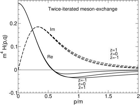
Figure 3: Real and imaginary part of the twice-iterated scalar-boson exchange NN-scattering amplitude $H(p,q)$. For further notations, see Fig. 2.

Figure 4: Crossed two-boson exchange diagram, and diagrams related (partly) to the iteration of the irreducible one-loop potential $V_{2}(q)$ with one-boson exchange.

At two-loop order there are also the non-planar ladder diagrams shown in Fig. 4. These correspond (partly) to the iteration of the irreducible two-boson exchange (i.e. the one-loop potential) with the one-boson exchange. The complete one-loop potential arises from the (left) crossed two-boson exchange diagram in Fig. 4 and the irreducible part of the (left) box diagram in Fig. 1. Both pieces together lead to the following result for the (static) one-loop potential  in momentum space:

$$V_{2}(q)={2g^{4}\over\pi^{2}}\,\vec{\tau}_{1}\cdot\vec{\tau}_{2}\,{1\over q\sqrt{4m^{2}+q^{2}}}\ln{q+\sqrt{4m^{2}+q^{2}}\over 2m}\,.$$ (9)

Our sign convention is chosen here such that the (static) one-boson exchange reads: $V_{1}(q)=g^{2}\,\vec{\tau}_{1}\cdot\vec{\tau}_{2}\,(m^{2}+q^{2})^{-1}$. It is interesting to note here that modulo their isospin factors $3\pm 2\vec{\tau}_{1}\cdot\vec{\tau}_{2}$ the crossed box diagram and the irreducible part of the planar box diagram are equal but with opposite sign in the limit $M\to\infty$ (for further details on that fact, see sect. 4.2 in ref.[6]). The coordinate space potential corresponding to Eq.(9) can be expressed through a modified Bessel function: $\widetilde{V}_{2}(r)=-g^{4}\vec{\tau}_{1}\cdot\vec{\tau}_{2}\,K_{0}(2mr)/2\pi^{3}r$.

Now we are in the position to calculate also the iteration of the (static) one-loop two-boson exchange potential with the one-boson exchange:

$$T_{3}^{\times}(p,q)={g^{6}M\over 2\pi^{3}}(3-2\vec{\tau}_{1}\cdot\vec{\tau}_{2})\,J(p,q)\,.$$ (10)

Unitarity determines again the imaginary part of the complex-valued amplitude $J(p,q)$ as:

$${\rm Im}\,J(p,q) = \int_{0}^{2p}dk\,\ln{k+\sqrt{4m^{2}+k^{2}}\over 2m}\,\bigg{\{}(4m^{2}+k^{2})$$

$$\times\Big{[}m^{4}p^{2}+m^{2}(2p^{2}(q^{2}+k^{2})-q^{2}k^{2})+p^{2}(q^{2}-k^{2})^{2}\Big{]}\bigg{\}}^{-1/2}\,,$$

and the real part Re $J(p,q)$ follows from an unsubtracted dispersion relation analogous to Eq.(5). The value at threshold $p=q=0$ is again calculable analytically, with the result:

$$m^{3}J(0,0)=\int_{2}^{\infty}{2\,dx\over x(x+1)\sqrt{x^{2}-4}}=\pi\bigg{(}{1\over 2}-{2\sqrt{3}\over 9}\bigg{)}\,,$$ (12)

where we have made use of the spectral function representation [6] of the (static) one-loop potential $V_{2}(q)$ written in Eq.(9).

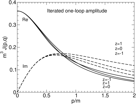
Figure 5: Real and imaginary part of the NN-scattering amplitude $J(p,q)$ generated by iterating the (static) irreducible one-loop potential with the one-boson exchange. For further notations, see Fig. 2.

In Fig. 5 we show the real and imaginary part of the (dimensionless) iterated one-loop amplitude $m^{3}J(p,q)$ versus the center-of-mass momentum $p$ in the region $0\leq p\leq 2m$. The real part displays only a minor dependence on the scattering angle, which is more pronounced for the imaginary part. Another noticeable feature is that the real part stays positive throughout and that the decrease of the amplitudes with increasing momentum $p$ is slower in comparison to $G(p,q)$ and $H(p,q)$ shown Figs. 2,3. The latter property has to do with the presence of the larger mass scale $2m$ in the (static) one-loop potential $V_{2}(q)$.

Figure 6: Crossed three-boson exchange diagrams. The dashed lines represent the isovector-scalar boson of mass $m$.

At two-loop order there are in addition the three crossed three-boson exchange diagrams shown in Fig. 6. These build up together with the irreducible parts of the two-loop ladder diagrams in Figs. 1,4 the (irreducible) three-boson exchange potential. The separation of a two-loop ladder diagram into twice-iterated $(\sim M^{2})$, once-iterated $(\sim M^{1})$, and nonrelativistic irreducible components $(\sim M^{0})$ is defined by the expansion of the corresponding Feynman amplitude in powers of the reciprocal nucleon mass $1/M$. For that one integrates first the product of light boson propagators $(l_{j}^{2}-m^{2}+i0^{+})^{-1}$ and heavy nucleon propagators $2M(p_{j}^{2}-M^{2}+i0^{+})^{-1}$ over the loop-energies $l^{0}_{1,2}$ via residue calculus and then expands in powers of $1/M$. This way we find that modulo their isospin factors $7\vec{\tau}_{1}\cdot\vec{\tau}_{2}\pm 6$ the irreducible part of the right (3-rung ladder) diagram  in Fig. 1 agrees with that of the left diagram in Fig. 6 [8]. Discarding again the isospin factors $7\vec{\tau}_{1}\cdot\vec{\tau}_{2}\pm 6$ and $-\vec{\tau}_{1}\cdot\vec{\tau}_{2}\pm 6$ we deduce furthermore that the total sum of the three crossed three-boson exchange diagrams in Fig. 6 is equal to the difference between the right (middle) crossed diagram in Fig. 6 and the irreducible part of the right (middle) ladder diagram in Fig. 4. Putting back the isospin factors and using the four relations between the irreducible parts of the six two-loop diagrams, we find for the isoscalar component of the (static) three-boson exchange potential in momentum space:

$$V_{3}(q)^{(is)}=-g^{6}\int{d^{3}l_{1}d^{3}l_{2}\over(2\pi)^{6}}\,{12\over\omega_{1}^{2}\omega_{2}^{4}\omega_{3}^{2}}=-{3g^{6}\over 8\pi^{2}m\,q}\,\arctan{q\over 3m}\,,$$ (13)

where we have made use of the results derived in the appendix of ref.[8]. The quantities $\omega_{j}=\sqrt{m^{2}+\vec{l}_{j}^{\,2}}$ denote the on-shell energies of the three exchanged scalar-isovector bosons, where $\vec{l}_{3}=\vec{l}_{1}+\vec{l}_{2}+\vec{q}$. The corresponding potential in coordinate space is repulsive and can be expressed by a simple exponential function: $\widetilde{V}_{3}(r)^{(is)}=3g^{6}e^{-3mr}/(32\pi^{3}mr^{2})$. The isovector part of the (irreducible) three-boson exchange potential proportional to $\vec{\tau}_{1}\cdot\vec{\tau}_{2}$ reads on the other hand:

$$V_{3}(q)^{(iv)}=g^{6}\int{d^{3}l_{1}d^{3}l_{2}\over(2\pi)^{6}}\,{4\over\omega_{1}^{3}\omega_{2}^{3}\omega_{3}}\bigg{[}{2\omega_{2}\over(\omega_{1}+\omega_{3})^{2}}+{1\over\omega_{1}+\omega_{2}+\omega_{3}}\bigg{]}\,.$$ (14)

At zero momentum transfer $q=0$ the six-dimensional integral in Eq.(14) can be evaluated analytically and the result $(6\pi m)^{-2}$ is found. For a numerical evaluation of the isovector potential $V_{3}(q)^{(iv)}$ the representation in Eq.(14) is not best suited. A better representation is obtained by introducing Feynman parameters for each four-dimensional loop integral and performing the elementary integrations over some of the Feynman parameters. After several skilful transformations we arrive at the following very handy double-integral representation:

$$V_{3}(q)^{(iv)} = {g^{6}\over 4\pi^{4}}\int_{0}^{1}\!\!dx\int_{0}^{\infty}\!\!dy\,\bigg{\{}1-\sqrt{y}\arctan{1\over\sqrt{y}}\bigg{\}}$$

$$\times\Big{[}m^{2}(x^{2}+xy+y+y^{2})+q^{2}x(1-x)y\Big{]}^{-1}\,.$$

In this form the $dx$-integral could even be solved in terms of square-root and arctangent or logarithmic functions (depending on the sign of a radicand). The associated coordinate space potential $\widetilde{V}_{3}(r)^{(iv)}$ can now also be computed easily. One just has to replace the polynomial inside the square brackets in Eq.(15) by the expression $-4\pi rx(1-x)y\exp\{mr[(x^{2}+xy+y+y^{2})/(x(1-x)y)]^{1/2}\}$. In the first and second row of Table I we have collected numerical values which display the dropping of the isoscalar and isovector three-boson exchange potentials $V_{3}(q)^{(is,iv)}$ with the momentum transfer $q$. In each case we have divided $V_{3}(q)^{(is,iv)}$ by the corresponding value at $q=0$. For comparison, we give in the third row the analogous ratios for the one-loop two-boson exchange potential $V_{2}(q)$ written down in Eq.(9). One observes that the isovector three-boson exchange potential drops somewhat faster than its isoscalar counterpart. This decrease is however weak in comparison to that of the two-boson exchange potential, mainly due to the different mass scales ($3m$ versus $2m$) involved. As an aside, we note that for a scalar-isoscalar boson the (static) irreducible two-boson and three-boson exchange potentials would both vanish identically: $V_{2}(q)=V_{3}(q)=0$. The latter zero-result follows from the relations between the irreducible parts of the six three-boson exchange two-loop diagrams, mentioned above.

$q/m$	1	2	3	4	5	6	7	8	9	10
3-isoscalar	0.965	0.882	0.785	0.695	0.618	0.554	0.500	0.455	0.416	0.384
3-isovector	0.957	0.856	0.739	0.633	0.544	0.471	0.412	0.363	0.322	0.289
one-loop	0.861	0.623	0.442	0.323	0.245	0.192	0.154	0.127	0.107	0.091
2-isoscalar	0.927	0.785	0.655	0.554	0.476	0.416	0.369	0.331	0.300	0.275
2-isovector	0.960	0.874	0.783	0.704	0.637	0.581	0.534	0.494	0.460	0.430

Table I: First and second row: The isoscalar and isovector three-boson exchange potentials Eqs.(13,15) versus the momentum transfer $q$. The respective values at $q=0$ have been divided out. The third row gives the analogous ratios for the one-loop two-boson exchange potential Eq.(9). The fourth and fifth row correspond to the two-boson-exchange potentials with one-loop vertex corrections written in Eqs.(18,19).

Figure 7: Two-boson exchange diagrams with one-loop vertex corrections. The diagrams with uncrossed boson lines and the role of both nucleons interchanged are not shown.

For the sake of completeness (at two-loop order in the nonrelativistic approximation) we consider also the two-boson exchange diagrams with vertex corrections shown in Fig. 7. In order to evaluate them we make use of the methods outlined in ref.[9]. From the one-loop corrections (beyond mass and coupling constant renormalization) to the isospin-even and isospin-odd boson-nucleon scattering amplitudes:

$$T^{+}_{bN}(\omega)={2g^{4}\over\pi\omega^{2}}\Big{(}m-\sqrt{m^{2}-\omega^{2}}\Big{)}\,,\qquad T^{-}_{bN}(\omega)={2g^{4}\over\pi^{2}\omega^{2}}\bigg{[}\omega-\sqrt{m^{2}-\omega^{2}}\arcsin{\omega\over m}\bigg{]}\,,$$ (16)

one can calculate (via unitarity) the spectral functions Im $V_{2}(i\mu)$. These mass spectra determine then the two-boson exchange potentials in momentum space through an unsubtracted dispersion relation:

$$V_{2}(q)={2\over\pi}\int_{2m}^{\infty}d\mu\,{\mu\,{\rm Im}V_{2}(i\mu)\over\mu^{2}+q^{2}}\,.$$ (17)

We find for the isoscalar part of the two-boson exchange potential with one-loop vertex corrections:

$$V_{2}(q)^{(is)}_{vc}={3g^{6}\over 4\pi^{2}m\,q}\arctan{q\over 2m}\,,$$ (18)

whose associated coordinate space representation is a simple exponential function: $\widetilde{V}_{2}(r)^{(is)}_{vc}=-3g^{6}\,e^{-2mr}/(16\pi^{3}mr^{2})$. The isovector component proportional to $\vec{\tau}_{1}\cdot\vec{\tau}_{2}$ reads on the other hand:

$$V_{2}(q)^{(iv)}_{vc}={2g^{6}\over\pi^{4}m\,q}\int_{1}^{\infty}{dx\,x\over(x^{2}-1)^{2}}\Big{[}\sqrt{x^{2}-1}-x\ln(x+\sqrt{x^{2}-1})\Big{]}\arctan{q\over 2mx}\,,$$ (19)

with the value $-g^{6}/(2\pi^{4}m^{2})$ at zero momentum transfer $q=0$. In order to obtain the associated coordinate space potential one just has to replace $q^{-1}\arctan(q/2mx)$ in Eq.(19) by the expression $-e^{-2mrx}/(4\pi r^{2})$. The numbers in the fourth and fifth row of Table I display the dependence of these two-boson exchange potentials with one-loop vertex corrections $V_{2}(q)^{(is,iv)}_{vc}$ on the momentum transfer $q$. One observes a slow decrease similar to that of the irreducible three-boson exchange potentials.

In summary we have calculated in this work all nonrelativistic contributions from scalar-isovector boson-exchange between nucleons at one- and two-loop order (including vertex corrections). At one loop order these contributions consist of the once-iterated boson-exchange amplitude and the irreducible two-boson exchange potential. At two-loop order one has the complex-valued scattering amplitudes related to the twice-iterated boson-exchange and the iteration of the one-loop potential with the one-boson exchange as well as the irreducible three-boson exchange potentials and the two-boson exchange potentials with one-loop vertex corrections. In each case we have given analytical expressions involving only the minimum number of integrations (to be done numerically). The present results could be useful for phase-shift analyses, few- and many-body calculations, etc. The applied methods can be straightforwardly generalized to the pseudoscalar-isovector pion with its spin- and momentum-dependent couplings to the nucleon. The number of amplitudes and diagrammatic contributions to each amplitude increases however drastically by several orders of magnitude. Work along these lines is in progress [7]. In passing we have to point out that there exist still other two-loop contributions which also scale as $g^{6}M^{0}$. These complex-valued amplitudes correspond either to the iteration of the relativistic $1/M$-correction to the one-loop potential with the one-boson exchange, or to relativistic $1/M^{2}$-correction to the twice-iterated boson-exchange. More work is necessary in order to isolate, classify, and analytically compute these relativistic correction terms.

References

- [1] E. Epelbaum, Prog. Part. Nucl. Phys. (2006), in print; nucl-th/0509032.
- [2] E. Epelbaum, W. Glöckle, and Ulf-G. Meißner, Nucl. Phys. A747, 362 (2005); and refs. therein.
- [3] D.R. Entem and R. Machleidt, Phys. Rev. C68, 041001 (2003); and refs. therein.
- [4] J.A. Oller, E. Oset, and A. Ramos, Prog. Part. Nucl. Phys. 45, 157 (2000); and refs. therein.
- [5] J.A. Oller, Nucl. Phys. A725, 85 (2003).
- [6] N. Kaiser, R. Brockmann, and W. Weise, Nucl. Phys. A625, 758 (1997).
- [7] N. Kaiser, J.A. Oller, and M.A. Perez, work in progress.
- [8] N. Kaiser, Phys. Rev. C62, 024001 (2000).
- [9] N. Kaiser, Phys. Rev. C64, 057001 (2001).