Quasiclassical description of bremsstrahlung accompanying
$\boldsymbol{\alpha}$ decay including quadrupole radiation

Abstract

We present a quasiclassical theory of $\alpha$ decay accompanied by bremsstrahlung with a special emphasis on the case of ²¹⁰Po, with the aim of finding a unified description that incorporates both the radiation during the tunneling through the Coulomb wall and the finite energy $E_{\gamma}$ of the radiated photon up to $E_{\gamma}\sim Q_{\alpha}/\sqrt{\eta}$, where $Q_{\alpha}$ is the $\alpha$-decay $Q$-value and $\eta$ is the Sommerfeld parameter. The corrections with respect to previous quasiclassical investigations are found to be substantial, and excellent agreement with a full quantum mechanical treatment is achieved. Furthermore, we find that a dipole-quadrupole interference significantly changes the $\alpha$-$\gamma$ angular correlation. We obtain good agreement between our theoretical predictions and experimental results.

I Introduction

A characteristic feature of the $\alpha$ decay process is the quantum mechanical tunneling Ga1929 through the so-called Coulomb wall generated by the electrostatic interaction of the $\alpha$ particle with the constituent protons of the daughter nucleus. Bremsstrahlung in $\alpha$ decay is intriguing because of the classically incomprehensible character of radiation emission during the tunneling process. Considerable attention has therefore been devoted to both experimental DAEtAl1994brems ; KaEtAl1997 ; Eremin2000 ; KaEtAl2000 ; KaEtAl1997jpg as well as theoretical investigations DyGo1996 ; PaBe1998 ; Dy1999 ; TaEtAl1999 ; Tk1999 ; Tk1999jetp ; BPZ1999 ; MaOl2003 ; MaBe2004 , with the aim of elucidating the role of tunneling during the emission process. It is necessary to emphasize, however, that the term “radiation during the tunneling process” has a restricted meaning as the wavelength of the photon is much larger than the width of the tunneling region and even larger than the main classical acceleration region. It is therefore not possible to identify the region where the photon was emitted. Besides, it is possible to write the matrix element of bremsstrahlung in different forms using operator identities. As a result, the integrands for the matrix element, as well as the relative contributions of the regions of integration, will be different depending on the operator identities used, although the total answer remains, of course, the same. This was demonstrated, e.g., by Tkalya in Refs. Tk1999 ; Tk1999jetp .

In the present paper, we revisit the theory of bremsstrahlung in the $\alpha$ decay of a nucleus with a special emphasis on the quasiclassical approximation. The applicability of this approximation is ensured by the large value of the Sommerfeld parameter $\eta$ (see below). We investigate the range of validity of the result obtained by Dyakonov Dy1999 and show that it is restricted by the condition $x\ll 1/\sqrt{\eta}$ where $x=E_{\gamma}/Q_{\alpha}$ (here, $E_{\gamma}$ is the photon energy, and $Q_{\alpha}$ is the $\alpha$-decay $Q$-value). Our quasiclassical result has no such a restriction although we assume $x\ll 1$. It is consistent with the results of both Dyakonov Dy1999 and Papenbrock and Bertsch PaBe1998 in limiting cases. For the experimentally interesting case of the $\alpha$ decay of ${}^{210}{\rm Po}$, our result is valid with high accuracy up to $x\sim 0.1$.

Another subject investigated here is the angular distribution of emitted photons. The $\alpha$ particle, initially in an $S$ state, may undergo a dipole transition to a $P$ final state, or a quadrupole transition to a $D$ state. While the quadrupole contribution is parametrically suppressed for small photon energies, the effective charge prefactor for the quadrupole contribution is large. The dipole-quadrupole interference term vanishes after angular averaging, but gives a significant contribution to the differential photon emission probability, resulting in a substantial deviation from the usually assumed dipole emission characteristics.

Very recently, the results of our high-statistics measurement of bremsstrahlung emitted in the $\alpha$ decay of ²¹⁰Po have been published, see Ref. ourexp . Due to the limited solid-angle coverage of the detectors used in this experiment, it was necessary to account for the $\alpha$-$\gamma$ angular correlation. Taking into account the contributions of the dipole and quadrupole amplitudes in the data analysis, as derived in the present paper, good overall agreement between theory and experiment is observed.

This paper is organized in four sections. In Sec. II, we investigate the leading dipole contribution to the differential bremsstrahlung probability and evaluate the corresponding amplitude in the quasiclassical approximation. The quadrupole contribution to the amplitude and its interference with the dipole part is analyzed in Sec. III. Conclusions are drawn in Sec. IV. Two appendices provide details on the methods used in the calculations.

II DIPOLE EMISSION

II.1 Emission Probability

It was shown in Ref. PaBe1998 that the differential bremsstrahlung probability $dP/dE_{\gamma}$ as a function of the energy $E_{\gamma}$ of the radiated photon in the dipole approximation has the form

$$\frac{dP}{dE_{\gamma}}=\frac{4\,e^{2}Z_{\rm eff}^{2}}{3\,\mu^{2}\,E_{\gamma}}\,\left|{\cal M}\right|^{2}\,,\qquad{\cal M}=\left<R_{f}\left|\partial_{r}V\right|R_{i}\right>\,,$$ (1)

where natural units with $\hbar=c=\epsilon_{0}=1$ are applied throughout the paper, $e$ is the proton charge and $\mu$ is the reduced mass of the combined system of $\alpha$ particle and daughter nucleus, $V\equiv V(r)=z(Z-z)\alpha/r$ is the potential of the daughter nucleus felt by the $\alpha$ particle. The functions $R_{i}$ and $R_{f}$ are the radial wave functions of the initial and final states corresponding to the angular momenta $l=0$ and $l=1$, respectively (see App. B). The effective charge for a dipole interaction between an $\alpha$ particle with charge number $z=2$ and mass number $4$ emitted from a parent nucleus with charge number $Z$ and mass number $A$ is (see also App. A)

$$Z_{\rm eff}=Z^{(1)}_{\rm eff}\approx\frac{2\,A-4\,Z}{A}=\frac{2}{5}\,,$$ (2)

where the latter value is relevant for the experimentally interesting case of the $\alpha$ decay of ${}^{210}{\rm Po}$ ($Z=84$). Evaluating the effective charge with accurate values for the masses of the alpha particle and the daughter nucleus (²⁰⁶Pb, $Z=82$), as given in Ref. Fi1996 yields a value of $Z^{(1)}_{\rm eff}=0.399$.

In the present paper, we calculate the matrix element ${\cal M}$ in the quasiclassical approximation taking into account the first correction of the order ${\cal O}(\eta^{-1})$, and the corresponding result is given below in Eq. (8). However, before presenting and discussing our formula for the matrix element ${\cal M}$, let us briefly review several results for ${\cal M}$ obtained earlier in the quasiclassical approximation. These are illustrative with respect to their range of applicability and with respect to the importance of the tunneling contribution.

II.2 Dipole Transition Matrix Element

Various approximations have been applied for the evaluation of the matrix element $\cal M$ in Eq. (1) Dy1999 ; PaBe1998 ; TaEtAl1999 ; Tk1999 ; Tk1999jetp . The approximations are intertwined with the identification of particular contributions to the real and imaginary parts of the matrix element $\mathcal{M}$ due to “tunneling” and due to “classical motion” of the $\alpha$ particle.

We use the convention that the complex phase of the matrix element $\cal M$ should be chosen in such a way that it becomes purely real in the classical limit $E_{\gamma}\to 0$. Our definition of $\cal M$ is consistent with that used in Ref. Dy1999 and differs by a factor $\rm{i}$ from the definition used in Ref. PaBe1998 .

Equation (5) in the work of Papenbrock and Bertsch PaBe1998 contains a fully quantum mechanical result for the photon emission amplitude $\mathcal{M}$, expressed in terms of regular and irregular Coulomb functions, without any quasiclassical approximations. However, the physical interpretation of this result depends on a comparison with a quasiclassical approximation, as only such a comparison clearly displays the importance of the finite photon energy and the emission amplitude during tunneling. Papenbrock and Bertsch PaBe1998 therefore present and discuss a quasiclassical expression for the imaginary part of their matrix element (real part for our convention), ignoring the contribution from the tunneling process to the emission amplitude. Note that the quasiclassical expression of Papenbrock and Bertsch PaBe1998 provides a very good approximation for the imaginary part of their matrix element up to very large photon energies with $x\sim 0.6$.

In contrast, the quasiclassical result of Dyakonov Dy1999 is valid only for very small photon energies ($x\ll 1/\sqrt{\eta}$), but includes contributions from tunneling. Here, we unify the treatments of Refs. PaBe1998 ; Dy1999 and obtain a quasiclassical differential emission probability $dP/dE_{\gamma}$, which includes the effect of photon emission during the tunneling process and which is substantially more accurate for higher photon energies than that of Dyakonov Dy1999 .

The quasiclassical approximation for the wave functions of the system of an $\alpha$ particle and a daughter nucleus in the initial and final states is valid for large values of the Sommerfeld parameters $\eta_{i,f}=z(Z-z)e^{2}\mu/k_{i,f}$ with $k_{i}=\sqrt{2\mu Q_{\alpha}}$ and $k_{f}=\sqrt{2\mu(Q_{\alpha}-E_{\gamma})}$. The indices $i$ and $f$ are reserved for initial and final configurations throughout the paper. The value of $\eta_{i}$ for the decay of ²¹⁰Po, which is the experimentally most interesting nucleus, is $22.0$, while the $Q$-value is $Q_{\alpha}=5.40746\,{\rm MeV}$ Fi1996 .

If one neglects the contribution to the matrix element $\mathcal{M}$ from the region $r\lesssim r_{0}$, where $r_{0}$ is the nuclear radius, then one is consistent with the simple assumption for the potential as a square well for $r<r_{0}$ and a pure repulsive Coulomb potential for $r>r_{0}$. Implementing this procedure according to Papenbrock and Bertsch PaBe1998 , one obtains the following approximation for the real part $M$ of the matrix element of $\mathcal{M}$,

$$M=\mbox{Re}\,\cal M\approx \,\eta_{i}\,\sqrt{\frac{2\,k_{i}}{\pi\,k_{f}}}\,$$

$$\;\times\int_{0}^{\infty}\frac{dr}{r^{2}}\,F_{1}(\eta_{f},k_{f}r)\,F_{0}(\eta_{i},k_{i}r)\,.$$ (3)

Here, $F_{0}$ and $F_{1}$ are the regular Coulomb radial wave functions corresponding to angular momenta $l=0$ and $l=1$, respectively. The importance of the contribution of the region $r\lesssim r_{0}$ was discussed in Refs. PaBe1998 ; Dy1999 . For relatively small photon energies, which are interesting from an experimental point of view, this contribution is not significant, and we do not consider it in the present paper. For high photon energies, the contribution of the region $r\sim r_{0}$ can be important (see Ref. BPZ1999 ). The explicit form of $M$ is given by Eqs. (6) and (7) of Ref. PaBe1998 ; PaBe1998-misprint .

We have calculated the integral in Eq. (II.2) using quasiclassical wave functions, keeping the correction of order ${\cal O}(\bar{\eta}^{-1})$ and ignoring terms of order ${\cal O}(1/\bar{\eta}^{2})$ and higher in the expansion for large “mean” Sommerfeld parameter ${\bar{\eta}}=(\eta_{i}+\eta_{f})/2$. The result of such a quasiclassical calculation for the real part of $\cal M$ reads

$$\widetilde{M}= \sqrt{\frac{2\,k_{i}}{\pi\,k_{f}}}\,\frac{k_{i}\,k_{f}}{k_{i}+k_{f}}\,\frac{\eta_{i}}{\bar{\eta}}$$

$$\times\xi\,{\rm e}^{-\pi\xi/2}\,\left[-K_{{\rm i}\xi}^{\prime}(\xi)-\frac{1}{\bar{\eta}}\,K_{{\rm i}\xi}(\xi)\right]\,,$$ (4)

where $\xi=\eta_{f}-\eta_{i}$, and $K_{a}(b)$ is the modified Bessel function. The derivative is $K_{a}^{\prime}(b)=\frac{\partial}{\partial b}K_{a}(b)$. Papenbrock and Bertsch PaBe1998 also calculated the real part of the integral (II.2) in the quasiclassical approximation. Note, however, that their term of order ${\cal O}(\bar{\eta}^{-1})$ [see Eq. (14) of Ref. PaBe1998 ] contains an additional factor $\sqrt{3}/2$ in comparison to Eq. (II.2).

Figure 1 shows the ratio ${\rm Re}\,{\cal M}/\widetilde{M}=M/\widetilde{M}$ as a function of $x$ for $\eta_{i}=22.0$, corresponding to the case of ²¹⁰Po. Note that even at $x=0.3$, the deviation of the quasiclassical result with the correction ${\cal O}(\bar{\eta}^{-1})$ taken into account is less than $1\%$ (solid line), while without this correction ($\widetilde{M}^{0}$), the deviation is about $5\%$ (dashed line).

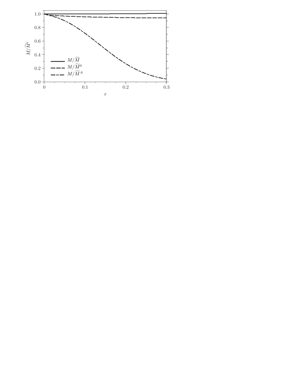
Figure 1: The ratio of $M=\mbox{Re}\,\cal M$, see Eq. (II.2), to various approximations, as a function of $x=E_{\gamma}/Q_{\alpha}$ for for the case of ²¹⁰Po ($\eta_{i}=22.0$). The solid line shows $M/\widetilde{M}$ with $\widetilde{M}$ taken from Eq. (II.2), illustrating the excellent agreement of the quasiclassical matrix element with the exact result in the range $x\leq 0.3$. For the dashed line we use $\widetilde{M}^{0}$, which is obtained from $\widetilde{M}$ by omitting the correction of order ${\cal O}(\bar{\eta}^{-1})$, showing a deviation of less than $5\%$. For the dash-dotted line the asymptotics $\widetilde{M}^{A}$ as given in Eq. (II.2) is used. The deviation of the latter curve from the others illustrates that the “$x\to 0$”-asymptotics is indeed only valid for $x\ll 1/\sqrt{\eta}$.

Strictly speaking, the validity of the evaluation of the transition matrix element (1) with the wave functions taken in the quasiclassical approximation requires special consideration (see §51 of Ref. LaLi1958 ) because of possibly noticeable contributions from the vicinities of the turning points. However, one can show that, for $\xi\ll\bar{\eta}$ (or $x\ll 1$), the contributions of the vicinities of the classical turning points ($r_{ci}=2\eta_{i}/k_{i}$ and $r_{cf}=2\eta_{f}/k_{f}$ in our case) are small. For $x\lesssim 1$, these contributions are no longer negligible.

For $x\ll 1$, we have $\xi=\eta_{i}\,(x/2+3x^{2}/8+\ldots)\,$. If $x^{2}\,\eta_{i}\ll 1$ (even if $x\,\eta_{i}\lesssim 1$), we can replace in (II.2) $\xi$ by $x\eta_{i}/2$ and make the substitution $\eta_{f}\to\eta_{i}$ and $k_{f}\to k_{i}$. As a result, we obtain the following asymptotics of $\widetilde{M}$:

$$\widetilde{M}^{A} =\frac{k_{i}}{\sqrt{2\pi}}\,\left(\frac{x\eta_{i}}{2}\right)\,{\rm e}^{-\pi x\eta_{i}/4}\,$$

$$\;\times\left[-K_{{\rm i}x\eta_{i}/2}^{\prime}\left(\frac{x\eta_{i}}{2}\right)-\frac{1}{\eta_{i}}\,K_{{\rm i}x\eta_{i}/2}\left(\frac{x\eta_{i}}{2}\right)\right]\,.$$ (5)

From the dash-dotted line of Fig. 1, we see that the ratio $M/\widetilde{M}^{A}$ deviates substantially from unity, illustrating that the applicability of Eq. (II.2) is indeed restricted to very small values of $x$.

Since

$$K_{i\nu}(x)=\exp(-\pi\nu/2)\int_{0}^{\infty}\cos(x\sinh t-\nu t)\,dt\,,$$ (6)

the quantity $\widetilde{M}^{A}$ without the ${\cal O}(\eta_{i}^{-1})$ correction exactly coincides with the real part of the amplitude ${\widetilde{\cal M}}_{\rm D}$ obtained by Dyakonov Dy1999 , where

$$\widetilde{\cal M}_{\rm D}= \;\frac{k_{i}}{\sqrt{2\pi}}\,J_{\rm D}\left(\frac{x\,\eta_{i}}{2}\right)\,,$$ (7a)

$$J_{\rm D}(y)= \;-{\rm i}\,y\exp(-\pi y)$$

$$\times\int_{0}^{\infty}dt\,\sinh(t)\,\exp[{\rm i}\,y\,(\sinh t-t)]\,,$$ (7b)

showing that this result is applicable only to very small photon energies. $\widetilde{\cal M}_{\rm D}$ contains both a real and an imaginary part and thus takes photon emission during tunneling into account. It was pointed out by Dyakonov Dy1999 that the imaginary part of $\widetilde{\cal M}_{\rm D}$ at $x\eta_{i}\sim 1$ is of the same order as the real part. For instance, in the case of the $\alpha$ decay of ²¹⁰Po with $\eta_{i}=22.0$, we have $x\,\eta_{i}\sim 1$ for $x\approx 0.05$. This indicates that the imaginary part of $\widetilde{\cal M}_{\rm D}$ is important.

Our quasiclassical approximation $\widetilde{\cal M}$ for the dipole transition matrix element $\cal M$ from Eq. (1), which includes the contributions from the tunneling of the $\alpha$ particle (we would like to refer to this result as the “unified result” in the following sections of the current paper) has the form:

$$\widetilde{\cal M}= \sqrt{\frac{2\,k_{i}}{\pi\,k_{f}}}\,\frac{k_{i}\,k_{f}}{k_{i}+k_{f}}\,\frac{\eta_{i}}{\bar{\eta}}\,\left[J(\xi)+\frac{1}{\bar{\eta}}J_{1}(\xi)\right]\,,$$ (8a)

$$J(y)= \;{\rm i}\,y\exp(-\pi y)$$

$$\times\int_{0}^{\infty}dt\,\sinh(t)\,\exp[{\rm i}\,y\,(t-\sinh t)]\,,$$ (8b)

$$J_{1}(y)= -y\exp(-\pi y)\,\int_{0}^{\infty}dt\,\exp[{\rm i}\,y\,(t-\sinh t)]\,.$$ (8c)

The derivation of Eqs. 8 (see App. B for more details) involves a shift of the integration region into the complex plane, which is needed to take the tunneling region into account in a quasi-classical treatment, as explained in DyGo1996 ; Dy1999 . Note that $J(y)$ is the complex conjugation of the function $J_{\rm D}(y)$ as defined in Eq. (7). Although this is irrelevant for the calculation of the bremsstrahlung emission probability, it is important for the dipole-quadrupole interference term discussed in Sec. III. The region of applicability of Eq. (8) is much wider than that of Eq. (7), because at small $x$ there is no additional restriction $x\ll 1/\sqrt{\eta}$ which may otherwise constitute a strong limitation at large value of $\eta$, as it was shown above. Moreover, Eq. (8) contains a correction ${\cal O}(\bar{\eta}^{-1})$, which is also essential.

Figure 2: The ratio $\mbox{Im}\,\widetilde{\cal M}/\mbox{Re}\,\widetilde{\cal M}$ for the case of ²¹⁰Po ($\eta_{i}=22.0$). The graph illustrates that the imaginary part of the matrix element $\widetilde{\cal M}$ is quite substantial even for moderate values of $x$.

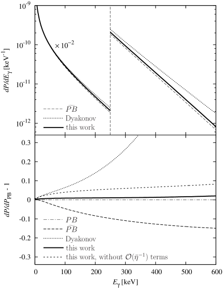
Figure 3: Differential branching ratio $dP/dE_{\gamma}$ for bremsstrahlung emission during $\alpha$ decay of ²¹⁰Po in units of inverse keV (top panel) and relative to the fully quantum mechanical calculation (PB) of Papenbrock and Bertsch PaBe1998 (bottom panel). The thick solid curve corresponds to our quasiclassical result, as given in Eq. (8). The other results are based on the quasiclassical treatment of Ref. PaBe1998 ($\widetilde{\rm PB}$), the semiclassical treatment of Dyakonov Dy1999 , and on Eq. (8) of the present work but neglecting the correction terms of order ${\cal O}(\bar{\eta}^{-1})$.

Our unified result (8) can be used with high accuracy up to $x\sim 0.3$. The real part of $\widetilde{\cal M}$ is identical to $\widetilde{M}$ given in Eq. (II.2) and is discussed already in detail above (see also Fig. 1). Figure 2 shows the ratio $\mbox{Im}\,\widetilde{\cal M}/\mbox{Re}\,\widetilde{\cal M}=\mbox{Im}\,\widetilde{\cal M}/\widetilde{M}$ as a function of $x$ at $\eta_{i}=22.0$, i.e. for the case of ${}^{210}{\rm Po}$. One can see that $\mbox{Im}\,\widetilde{\cal M}$ is not small in comparison to $\mbox{Re}\,\widetilde{\cal M}$. Thus, the imaginary part gives a noticeable contribution to $dP/dE_{\gamma}$ even for small $x$, and should not be neglected. This point was also emphasized in Refs. Dy1999 ; TaEtAl1999 .

II.3 Quantitative comparison of various quasiclassical results

As a last step, we compare in Fig. 3 the differential bremsstrahlung probability $dP/dE_{\gamma}$ for the bremsstrahlung accompanying $\alpha$ decay of ²¹⁰Po obtained with the use of our matrix element $\widetilde{\cal M}$ given in Eq. (8), the matrix element $\widetilde{M}$ [Eq. (II.2)], corresponding to the quasiclassical approach of Ref. PaBe1998 , and the matrix element $\widetilde{\cal M}_{\rm D}$ [Eq. (7)], to the full quantum mechanical formula given by Eq. (5) in PaBe1998 . A detailed comparison is shown in the bottom panel of Fig. 3 in the $\gamma$ energy range $0<E_{\gamma}<600$ keV. While the result of Dyakonov Dy1999 (dotted line) deviates roughly by a factor two at $E_{\gamma}=600$ keV, our result (thick solid line) agrees with the exact quantum mechanical treatment within about 2 % at this photon energy; the inclusion of the ${\cal O}(\bar{\eta}^{-1})$ correction is crucial in obtaining this agreement, as is evident from the supplementary curve in the bottom panel, where we omit the $J_{1}$ term from Eq. (8c). The quasiclassical approximation of Papenbrock and Bertsch PaBe1998 , obtained by neglecting the imaginary part of the matrix element (dashed line), deviates by more than 15 % at $E_{\gamma}=600$ keV. As expected, at low photon energies all results agree with each other.

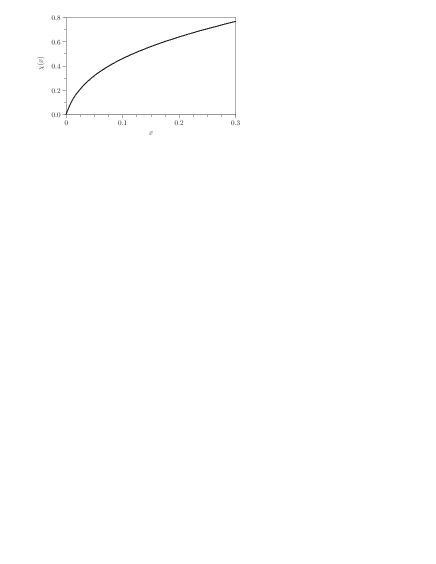
Figure 4: Interference term $\chi(x)$, defined in Eq. (11), for the bremsstrahlung accompanying $\alpha$ decay of ²¹⁰Po.

III QUADRUPOLE EMISSION

We are now concerned with the quadrupole component of the bremsstrahlung probability and the angular distribution of the radiation due to interference with the dipole components. The outgoing $\alpha$ particle defines an axis of symmetry. We therefore we may use $d\Omega=2\pi\sin\theta d\theta$ in order to describe the solid angle element of the photon spanning an infinitesimal range of polar angles $\theta$ with respect to the direction of the emitted $\alpha$-particle. We assume that a summation with respect to photon polarization is performed. Within the dipole approximation, Eq. (1) gives rise to an angular distribution of the form

$$\left.\frac{d^{2}P}{dE_{\gamma}d\Omega}\right|_{\rm dip}=\frac{e^{2}\left(Z^{(1)}_{\rm eff}\right)^{2}\sin^{2}\theta}{\pi\,\mu^{2}\,E_{\gamma}}\,\left|{\cal M}\right|^{2}\,,$$ (9)

where the index refers to the dipole approximation. Including the quadrupole term (see App. B), this formula should be generalized to

$$\frac{d^{2}P}{dE_{\gamma}d\Omega}= \;\frac{e^{2}\sin^{2}\theta}{\pi\mu^{2}E_{\gamma}}\left|Z_{\rm eff}^{(1)}\,{\rm e}^{{\rm i}\delta_{1}}\,{\cal M}\,+Z_{\rm eff}^{(2)}\,{\rm e}^{{\rm i}\delta_{2}}\,{\cal N}\,\cos\theta\right|^{2}$$

$$\,= \;\left.\frac{d^{2}P}{dE_{\gamma}d\Omega}\right|_{\rm dip}\,[1+\chi\,\cos\theta\,]+{\cal O}({\cal N}^{2})\,,$$ (10)

with

$$\chi= \;2\,\frac{Z_{\rm eff}^{(2)}}{Z_{\rm eff}^{(1)}}\,{\rm Re}\left(\frac{{\cal M}\,{\cal N}^{*}}{|{\cal M}|^{2}}\,{\rm e}^{{\rm i}(\delta_{1}-\delta_{2})}\right)\,,$$ (11)

where $\delta_{1}$ and $\delta_{2}$ are the Coulomb phases corresponding to the angular momenta $l=1$ and $l=2$, respectively. The effective quadrupole charge $Z^{(2)}_{\rm eff}$ is approximately given by (see App. A)

$$Z_{\rm eff}^{(2)}\approx 2+\frac{16(Z-A)}{A^{2}}=1.954\,$$ (12)

for the case of ${}^{210}{\rm Po}$, and is roughly five times larger than the dipole effective charge given in Eq. (2). Exact masses Fi1996 lead to the same result $Z_{\rm eff}^{(2)}=1.954$ (up to the last decimal digit indicated).

Calculating the quadrupole matrix element ${\cal N}$ within the quasiclassical approximation and keeping the leading in $1/\bar{\eta}$ term, we obtain

$$\widetilde{\cal N}= \;-\sqrt{\frac{2\,k_{i}}{\pi\,k_{f}}}\,\frac{k_{i}\,k_{f}}{k_{i}+k_{f}}\,\frac{\eta_{i}}{\bar{\eta}}\,v\,J_{1}(\xi)\,.$$ (13a)

We here neglect a parametrically suppressed next-to-leading order correction to the interference term, discussed in more detail in Appendix B, and we introduce the notation $v=\sqrt{2Q_{\alpha}/\mu}$, where $v$ approximately equals the final velocity of the $\alpha$ particle for bremsstrahlung emission with $x\ll 1$. For ${}^{210}{\rm Po}$, we have $v\approx 0.05$. Note that for a large Sommerfeld parameter $\eta_{f}$ we have

$${\rm e}^{{\rm i}\,(\delta_{2}-\delta_{1})}\approx{\rm i}+\frac{2}{\eta_{f}}\,.$$ (14)

Because of this “${\rm i}$” in the right-hand side of Eq. (14), the imaginary parts of the functions $J(\xi)$ and $J_{1}(\xi)$ become very important for the interference term. The quantity $\chi(x)$ defined in Eq. (11), which determines the relative magnitude of the interference term, vanishes for $x\to 0$ in the leading in $1/\bar{\eta}$ approximation as

$$\chi\approx\frac{\pi}{2}\,\frac{Z_{\rm eff}^{(2)}}{Z_{\rm eff}^{(1)}}\,v\,\eta_{i}\,x\,.$$ (15)

For ${}^{210}{\rm Po}$, this evaluates to $\chi\approx 8.64\,x$. Therefore, the value of the coefficient $\chi(x)$ becomes significant already at very small photon energies ($\chi\sim 0.1$ at $E_{\gamma}\sim 0.06$ MeV). The coefficient $\chi(x)$, calculated with our quasiclassical results $\widetilde{\cal M}$ and $\widetilde{\cal N}$, is plotted in Fig. 4 as a function of $x=E_{\gamma}/Q_{\alpha}$ for the experimentally interesting case of ${}^{210}{\rm Po}$.

When integrating Eq. (III) over the total solid angle, the interference term drops out and the remaining quadrupole contribution to the differential emission probability is of the order ${\cal O}(\widetilde{\cal N}^{2})$; for the case of ²¹⁰Po this contribution amounts to less than 1.5 % of the leading dipole term for photon energies up to 600 keV ($x\approx 0.1$).

IV Summary

In summary, using a quasiclassical approximation we have obtained an expression for the dipole bremsstrahlung probability during $\alpha$ decay which is in agreement with the full quantum mechanical treatment of Papenbrock and Bertsch PaBe1998 in a substantially wider region of the variable $x=E_{\gamma}/Q_{\alpha}$ in comparison with all previous quasiclassical results. Our amplitude given in Eq. (8) contains both real and imaginary parts and, thus, includes the contribution from bremsstrahlung during the tunneling process. Our results demonstrate that the latter contribution is not negligible even for rather small $x$. As an illustration of these statements, we have considered the experimentally important case of ²¹⁰Po.

Furthermore, we find the quasiclassical expression for the contribution of the interference term of the dipole and quadrupole components to the double differential bremsstrahlung probability (with respect to the energy and the solid angle of the photon). This contribution turns out to be significant. Because of obvious limitations to the solid angle that can be covered by detectors in a realistic experiment, the angular distribution needs to be considered in the analysis of the experimental data, even though the quadrupole term makes a negligible contribution to the bremsstrahlung probability after integration over the entire solid angle. Using the expression for the dipole and quadrupole amplitudes presented in this work, the data analysis in our recent experiment was performed as described in Ref. ourexp , and good overall agreement of our theoretical and experimental results was obtained (see Fig. 5 of Ref. ourexp ). We note, however, that a certain subtle question remains with respect to a next-to-leading order, nuclear model-dependent correction to the dipole-quadrupole interference term, as discussed in Appendix B. These questions leave room for further interesting investigations in the context of under-the-barrier emission of bremsstrahlung in $\alpha$ decay in the future.

Appendix A Effective charges

The purpose of this appendix (see also Eisenberg ) is to clarify how the effective charges in Eqs. (2) and (12) for the dipole and the quadrupole terms arise in the interaction of a two-body system (charges $eZ_{1}$ and $eZ_{2}$, masses $m_{1}$ and $m_{2}$, $e$ is the proton charge) with a photon of polarization $\bm{\epsilon}$ and wave vector $\bm{q}$, as given by the part of the Hamiltonian corresponding to emission of a photon,

$$H_{I}= -\frac{eZ_{1}}{m_{1}}\,\bm{\epsilon}^{*}\cdot\bm{p}_{1}\,\exp\left(-{\rm i}\,\bm{q}\cdot\bm{r}_{1}\right)$$

$$-\frac{eZ_{2}}{m_{2}}\,\bm{\epsilon}^{*}\cdot{\bm{p}}_{2}\,\exp\left(-{\rm i}\,\bm{q}\cdot\bm{r}_{2}\right)\,.$$ (16)

We define the total mass $M=m_{1}+m_{2}$, the reduced mass $\mu=m_{1}m_{2}/M$ , the center-of-mass coordinate $\bm{R}=(m_{1}/M)\bm{r}_{1}+(m_{2}/M)\bm{r}_{2}$, and the relative coordinate $\bm{r}=\bm{r}_{1}-\bm{r}_{2}$. Let $\bm{p}$ and $\bm{P}$ be the momenta corresponding to the coordinates $\bm{r}$ and $\bm{R}$, respectively. Then $\bm{p}_{1}=\bm{p}+(m_{1}/M)\bm{P}$ and $\bm{p}_{2}=-\bm{p}+(m_{2}/M)\bm{P}$. Writing the Hamiltonian (A) in the center-of-mass frame ($\bm{P}=0$) and performing its expansion over $|\bm{q}\cdot\bm{r}|\ll 1$ up to the first term, we obtain

$$H_{I}=-e\frac{\bm{\epsilon}^{*}\cdot\bm{p}}{\mu}\,\left[Z^{(1)}_{\rm eff}-{\rm i}\,Z^{(2)}_{\rm eff}\,\bm{q}\cdot\bm{r}\right]{\rm e}^{-{\rm i}\bm{q}\cdot\bm{R}}\,,$$ (17)

where the overall phase factor ${\rm e}^{-{\rm i}\bm{q}\cdot\bm{R}}$ can be safely ignored.

The effective charges are

$$Z^{(1)}_{\rm eff}= \frac{Z_{1}\,m_{2}-Z_{2}\,m_{1}}{m_{1}+m_{2}}\,,$$ (18)

$$Z^{(2)}_{\rm eff}= \frac{Z_{1}\,m_{2}^{2}+Z_{2}\,m_{1}^{2}}{(m_{1}+m_{2})^{2}}\,.$$ (19)

Appendix B Matrix elements

In this appendix we present some details of the derivation of our quasiclassical dipole (8) and quadrupole (13) matrix elements. The wave function of the final state has the form (see, e. g., §136 and §137 of LaLi1958 ):

$$\psi_{f}(\bm{r}) \equiv\psi^{(-)}_{\bm{k}_{f}}(\bm{r})$$

$$= \frac{1}{2k_{f}}\sum_{l=0}^{\infty}{\rm i}^{l}\,{\rm e}^{-{\rm i}\delta_{l}}\,(2l+1)\,R_{k_{f},\,l}(r)\,P_{l}(\bm{n}\cdot\bm{\lambda})\,,$$ (20)

where $\bm{n}=\bm{r}/r$, $\bm{\lambda}=\bm{k}_{f}/k_{f}$, $P_{l}$ are the Legendre polynomials, and

$$R_{k_{f},\,l}(r)=\frac{2}{r}F_{l}(\eta_{f},k_{f}r)$$ (21)

is the regular radial solution of the Schrödinger equation in a Coulomb field.

When comparing to Eq. (5) of Ref. PaBe1998 , it is evident that the ansatz (21) for the final-state wave function corresponds to the neglect of the contribution from the irregular solution in the Couloumb field, which given by the term $2r^{-1}G_{l}(\eta_{f},k_{f}r)\,\tan\alpha$ in the integral in Eq. (5) of Ref. PaBe1998 . The basis for our approximation (21) is as follows. The asymptotics of the wave function at $kr\gg 1$ is $2r^{-1}\sin(kr+f_{C}+\delta_{N})$, where $f_{C}$ corresponds to the asymptotics in a pure Coulomb field, and the phase shift $\delta_{N}$ is due to the nuclear potential, which has a size of the order of $r_{0}$. So, the asymptotic form of $R_{k_{f},l}(r)$ is proportional to $\cos(\delta_{N})F_{l}(\eta_{f},k_{f}r)+\sin(\delta_{N})G_{l}(\eta_{f},k_{f}r)$.

It follows from the quasiclassical approximation that the wave function at $r\ll r_{cf}\equiv r_{t}$, where $r_{t}=2\eta_{f}/(\mu v)$ is the classical turning point, is given by $F_{l}(\eta_{f},k_{f}r)\propto\exp[-2\sqrt{2\mu v\eta_{f}}\,(\sqrt{r_{t}}-\sqrt{r})]$. Therefore, $\delta_{N}\propto\exp[-8\eta_{f}]\ll 1$, and one is therefore led to the tentative conclusion that the term with the $G$ function should be entirely negligible. However, one might still object that the function $G$ is exponentially large at $r\ll r_{t}$, namely $G_{l}(\eta_{f},k_{f}r)\propto\exp[2\sqrt{2\mu v\eta_{f}}\,(\sqrt{r_{t}}-\sqrt{r})]$. In order to convince ourselves that the contribution from the $G$ functions is indeed small, let us consider as an example the term $\sin(\delta_{N})G_{0}(\eta_{i},k_{i}r)\,G_{l}(\eta_{f},k_{f}r)$. This term is proportional to $\exp[-4(\eta_{f}-\eta_{i})]\exp(-4\sqrt{2\mu v\bar{\eta}}\sqrt{r})$. Therefore, the main contribution to the transition matrix element from this term is given by the region $r\sim 1/(32\mu\eta v)=1/(32\mu(zZ\alpha))\ll r_{0}$. This contribution is indeed small, and we can safely use the approximation (21) for the final state of the $\alpha$ particle.

The wave function of the initial state is given by an $S$ state which consists of an outgoing wave at $r\to\infty$,

$$\psi_{i}(\bm{r})=\frac{R_{0}(r)}{\sqrt{4\pi}}=\frac{1}{\sqrt{4\pi}\,r}\,[G_{0}(\eta_{i},k_{i}r)+{\rm i}\,F_{0}(\eta_{i},k_{i}r)]\,.$$ (22)

Substituting the wave functions into the transition matrix element and taking the integrals over the angular parts of the $\alpha$ particle wave functions, we obtain

$$\left<f|H_{I}|i\right>=-\frac{\sqrt{4\pi}\,e\,\eta_{i}\,k_{i}}{2k_{f}\,\mu^{2}\omega}\,\bm{\epsilon}\cdot\bm{\lambda}$$

$$\times\Bigl{\{}Z^{(1)}_{\rm eff}e^{{\rm i}\delta_{1}}\int\limits_{0}^{\infty}{\rm d}rR_{k_{f},\,1}(r)R_{0}(r)$$

$$+Z^{(2)}_{\rm eff}e^{{\rm i}\delta_{2}}\,\cos\theta\,\int\limits_{0}^{\infty}{\rm d}rR_{k_{f},\,2}(r)\left[r\omega+\frac{9}{\mu r}\right]R_{0}(r)\Bigr{\}}\,,$$ (23)

where $\theta$ is the angle between the vectors $\bm{q}$ and $\bm{\lambda}$, $\omega=|\bm{q}|=E_{\gamma}$. Defining ${\cal M}$ and ${\cal N}$ as

$${\cal M}= -{\rm i}\eta_{i}\sqrt{\frac{k_{i}}{2\pi k_{f}}}\int_{0}^{\infty}drR_{k_{f},\,1}(r)R_{0}(r)\,,$$ (24)

$${\cal N}= -{\rm i}\eta_{i}\sqrt{\frac{k_{i}}{2\pi k_{f}}}\,\int_{0}^{\infty}drR_{k_{f},\,2}(r)\left(\frac{9}{\mu r}+r\omega\right)R_{0}(r)\,,$$ (25)

and taking into account that the sum over the photon polarizations gives $\sum|\bm{\epsilon}\cdot\bm{\lambda}|^{2}=\sin^{2}\theta$, we obtain the double-differential bremsstrahlung probability as

$$\frac{d^{2}P}{dE_{\gamma}d\Omega}= \frac{e^{2}}{\pi\mu^{2}E_{\gamma}}\sin^{2}\theta\,|{\cal C}|^{2}\,,$$

$${\cal C}= Z^{(1)}_{\rm eff}e^{{\rm i}\delta_{1}}{\cal M}+Z^{(2)}_{\rm eff}e^{{\rm i}\delta_{2}}{\cal N}\cos\theta\,,$$ (26)

in agreement with Eq. (III). Then we use the quasiclassical approximation for the radial part of the wave functions (see, e.g., § 48, 49 of Ref. LaLi1958 ). The matrix elements with the quasiclassical radial wave functions have been calculated using methods described in detail in Ref. Alder56 . Although these methods are in principle well known, we present here some details of the calculation.

Let us consider first the contribution $I_{0}$ of the classically allowed region to the matrix element

$$I_{1}=\int\limits_{0}^{\infty}{\rm d}rR_{k_{f},\,1}(r)R_{0}(r)$$ (27)

Using the standard quasiclassical wave function and assuming $x\ll 1$, we obtain

$$I_{0} \approx -\frac{1}{4i\bar{\eta}}\int\limits_{0}^{\infty}\frac{d\vartheta}{\cosh^{2}(\vartheta/2)}\mbox{e}^{i\xi(\sinh\vartheta+\vartheta)}$$ (28)

$$\left\{1+i\frac{b_{1}-b_{0}}{2\bar{\eta}}\tanh(\vartheta/2)\right\}$$

$$= \frac{\xi}{2\bar{\eta}}\Bigg{(}\int\limits_{0}^{\infty}d\vartheta\sinh(\vartheta)\,\mbox{e}^{i\xi(\sinh\vartheta+\vartheta)}$$

$$-\frac{i}{\bar{\eta}}\int\limits_{0}^{\infty}d\vartheta\,\mbox{e}^{i\xi(\sinh\vartheta+\vartheta)}\Bigg{)}\,,$$

where $b_{l}=(l+1/2)^{2}$ and the second expression is obtained after an integration by parts. According to Dy1999 , the classically forbidden part can be incorporated by shifting the integration contour for $\vartheta$ into the complex plane, via the replacement $\vartheta\to\vartheta+i\pi$. As a result we arrive at

$$I_{1} = -\frac{\xi}{2\bar{\eta}}\,\mbox{e}^{-\pi\xi}\Bigg{(}\int\limits_{0}^{\infty}d\vartheta\sinh(\vartheta)\,\mbox{e}^{i\xi(\sinh\vartheta-\vartheta)}$$ (29)

$$+\frac{i}{\bar{\eta}}\int\limits_{0}^{\infty}d\vartheta\,\mbox{e}^{i\xi(\sinh\vartheta-\vartheta)}\Bigg{)}\,.$$

Similarly, the leading in $1/\bar{\eta}$ contribution to the quadrupole amplitude is determined by the integral [see the second term in square brackets in Eq. (25)]

$$I_{21} = \int\limits_{0}^{\infty}{\rm d}rR_{k_{f},\,2}(r)r\omega R_{0}(r)$$ (30)

$$= \frac{iv\xi}{2\bar{\eta}}\mbox{e}^{-\pi\xi}\int\limits_{0}^{\infty}d\vartheta\,\mbox{e}^{i\xi(\sinh\vartheta-\vartheta)}\,.$$

The results (29) and (30) immediately verify Eqs. (8) and (13).

For the second contribution to the quadrupole amplitude, see Eq. (25),

$$I_{22} = \int\limits_{0}^{\infty}{\rm d}rR_{k_{f},\,2}(r)\frac{9}{\mu r}R_{0}(r),$$ (31)

we find that this term is suppressed by a factor $1/\bar{\eta}$. However, while $I_{21}$ vanishes in the limit of a small photon energy $x\to 0$, the contribution $I_{22}$ tends to a nonzero constant at $x=0$, i.e., even though $I_{22}$ is parametrically suppressed by a factor $1/{\bar{\eta}}$, it constitutes the dominant contribution to the dipole-quadrupole interference term at very small photon energies, due to its distinctive asymptotic behaviour.

A precise calculation of the $I_{22}$ contribution to the interference term is unfortunately hampered by the fact that the region of integration around $r\sim r_{0}$ gives an important contribution to the value of $I_{22}$ due to the inverse power of $r$ in the integrand, which thus makes the value of $I_{22}$ nuclear model-dependent. In the data analysis of our recent experiment ourexp , we therefore did not include the parametrically suppressed term $I_{22}$. While good overall agreement between experiment and theory was obtained in this way (see Fig. 5 of Ref. ourexp ), the agreement is better at photon energies $E_{\gamma}\geq 250\,{\rm keV}$ as compared to photon energies below this region. As the region of small $E_{\gamma}$ coincides with the region where the $I_{22}$ term might contribute to the dipole-quadrupole interference term, its significance cannot be completely ruled out at present.

References

- (1) G. Gamow, Nature (London) 123, 606 (1929).
- (2) A. D’Arrigo, N. Eremin, G. Fazio, G. Giardina, M. G. Glotova, T. V. Klochko, M. Sacchi, and A. Taccone, Phys. Lett. B 332, 25 (1994).
- (3) J. Kasagi, H. Yamazaki, N. Kasajima, T. Ohtsuki, and H. Yuki, Phys. Rev. Lett. 79, 371 (1997).
- (4) N.V. Eremin, G. Fazio, and G. Giardina, Phys. Rev. Lett. 85, 3061 (2000).
- (5) J. Kasagi, H. Yamazaki, N. Kasajima, T. Ohtsuki, and H. Yuki, Phys. Rev. Lett. 85, 3062 (2000).
- (6) J. Kasagi, H. Yamazaki, N. Kasajima, T. Ohtsuki, and H. Yuki, J. Phys. G 23, 1451 (1997).
- (7) M. I. Dyakonov and I. V. Gornyi, Phys. Rev. Lett. 76, 3542 (1996).
- (8) T. Papenbrock and G. F. Bertsch, Phys. Rev. Lett. 80, 4141 (1998).
- (9) M. I. Dyakonov, Phys. Rev. C 60, 037602 (1999).
- (10) N. Takigawa, Y. Nozawa, K. Hagino, A. Ono, and D. M. Brink, Phys. Rev. C 59, R593 (1999).
- (11) E. V. Tkalya, Phys. Rev. C 60, 054612 (1999).
- (12) E. V. Tkalya, Zh. Éksp. Teor. Fiz. 116, 390 (1999), [JETP 89, 208 (1999)].
- (13) C. A. Bertulani, D. T. de Paula, and V. G. Zelevinsky, Phys. Rev. C 60, 031602(R) (1999).
- (14) S. P. Maydanyuk and V. S. Olkhovsky, Prog. Theor. Phys. 109, 203 (2003).
- (15) S. P. Maydanyuk and S. V. Belchikov, Prob. At. Science and Technology 5, 19 (2004).
- (16) H. Boie, H. Scheit, U. D. Jentschura, F. Köck, M. Lauer, A. I. Milstein, I. S. Terekhov, and D. Schwalm, Phys. Rev. Lett. 99, 022505 (2007).
- (17) R. B. Firestone, Table of Isotopes (J. Wiley & Sons, New York, 1996).
- (18) In the notation of Eq. (7) of PaBe1998 , should be replaced by in the expression for (twice).
- (19) L. D. Landau and E. M. Lifshitz, Quantum Mechanics (Volume 3 of the Course of Theoretical Physics) (Pergamon Press, London, 1958).
- (20) J. M. Eisenberg and W. Greiner, Nuclear Theory Vol. 2: Excitation mechanisms of the nucleus, (North-Holland, Amsterdam, 1988), 3rd edition.
- (21) K. Alder, A. Bohr, T. Huus, B. Mottelson, and A. Winther, Rev. Mod. Phys., 28,432 (1956).