I Introduction

The capture of a negative muon from the atomic $1s$ orbit,

$$\mu^{-}+(Z,N)\rightarrow\nu_{\mu}+(Z-1,N+1)^{*}$$ (1)

is a semileptonic weak process that has been studied for a long time (see, e.g., the recent review Mrev or the earlier one by Walecka Wal and the classic by Mukhopadhyay Muk and the earlier references therein). The total capture rate has been measured for many stable nuclei; in some cases the capture rates on separated isotopes have been also determined Measday .

The nuclear response in muon capture is governed by the momentum transfer of the order of the muon mass. The phase space and the nuclear response favor lower nuclear excitation energies, thus the nuclear states in the giant resonance region dominate. Since the experimental data are quite accurate, and the theoretical techniques of evaluating the nuclear response in the relevant regime are well developed, it is worthwhile to see to what extent the capture rates are understood globally. Such a comparison may be viewed as a general test of our ability to describe semileptonic weak charged-current reactions with $q\sim m_{\mu}$ over a large range of nuclei, where $q$ is the momentum transfer and $m_{\mu}=105.6$ MeV is the muon mass.

The present work represents a first fully comprehensive theoretical evaluation of the total muon capture rate over the full range of nuclei where the experimental data are available. Previously, the muon capture rates for selected nuclei encompassing, however, a broad range of atomic charges, were calculated in Ref. Fearing . That paper was devoted mostly to the description of the radiative muon capture, and the total muon capture rates were a byproduct with only a limited agreement with the data. More along the lines of the present approach, Ref. Auer1 and Auer2 used a Hatree-Fock random phase approximation method and obtained good agreement with experiment, however only for a limited selection of nuclei. The local Fermi gas model was used successfully for the evaluation of the muon capture rate in selected nuclei in Ref. Chiang , and more recently in Ref. Nieves .

The present work is an extension of previous papers devoted to this issue Kolbe1 ; Kolbe2 . In Ref. Kolbe1 the capture rates for ¹²C, ¹⁶O and ⁴⁰Ca were evaluated using the continuum random phase approximation, and a very good agreement with the total rate was obtained. However, the residual interaction employed in Kolbe1 was adjusted to describe other observables in the cases of ¹²C and ¹⁶O. Moreover, it was necessary to quench the Gamow-Teller like (GT) partial capture rate leading to the $1^{+}$ ground state of ¹²B. In the later Ref. Kolbe2 heavier nuclei with $N>Z$, ^44,48Ca, ⁵⁶Fe, ⁹⁰Zr, and ²⁰⁸Pb were also included with a similar success. In Ref. Kolbe2 it has also been shown that for the calculation of muon capture rates the standard random phase approximation (SRPA) is essentially equivalent to the more computationally demanding continuum random phase approximation. Thus, the SRPA method is also used in the present study. In Ref. Zinner04 the SRPA approach has been used to study the muon capture rates to a long chain of calcium and tin isotopes.

One of the important issues when evaluating the response of nuclei to weak probes of relatively low energies is the problem of quenching of the corresponding strength. The evidence for quenching comes primarily from the analysis of the beta decay of the $(sd)$ shell Wildenthal as well as $(p,f)$ shell pf nuclei. In addition, the interpretation of the forward angle $(p,n)$ and $(n,p)$ charge-exchange reactions pn ; Langanke95 ; Martinez96 leads to the same conclusion. All such evidence, so far, is restricted to the GT strength and relatively low excitation energies. A convenient and customary way to account for this quenching is to use an ‘effective’ axial-vector coupling constant $g_{A}$, reducing it from its nominal value of $g_{A}=1.26$ to $g_{A}\sim 1$.

The evaluation of the muon capture rate, reported here, suggests that the quenching of $g_{A}$ is not needed to describe these data. (That conclusion was already reached in Refs.Kolbe1 ; Kolbe2 .) As stressed above, the mean excitation energy in muon capture is in the region of giant resonances of about 15 MeV (slowly decreasing with $A$ or $Z$), and the GT-like operators contribute very little in heavier nuclei where the neutrons and protons are in different oscillator shells. In lighter nuclei, for $N$ and $Z$ less than 40, the GT strength contributes, and is concentrated at low energy. Thus, in agreement with the evidence mentioned above, we quench this, and only this, part of the transition strength by a common factor $(0.8)^{2}=0.64$ Wildenthal .

The present work, and the evaluation of the muon capture in general, makes it possible to extend the study of quenching to higher multipoles, and correspondingly to higher nuclear excitation energies. Such processes, typically, depend primarily on the positions of the corresponding giant resonances and on the overall strength. Our conclusions, therefore, show that the SRPA method involving correlated particle-hole excitations, is capable of describing the inclusive semileptonic processes with momentum transfer $q$ of order $\sim m_{\mu}$ quite well. This is an important conclusion, applicable to a variety of practically important subjects, e.g. detection of supernova neutrinos or evaluation of the nuclear matrix elements for neutrinoless double beta decay.

The challenge of evaluating the muon capture rate in a wide variety of nuclei made it necessary to include several effects that were not usually included in analogous calculations. Since we needed to describe the bound muon in the $1s$ orbit well, we went beyond the usual calculation of the muon density at the site of the nucleus. First, we solved the Dirac equation in the field of the finite size nucleus numerically. We then used its wave function, taking into account that it is not constant between the origin and the nuclear surface. For high $Z$ values the muon is relativistic, and the ‘small’ $p_{1/2}$ component of its wave function is nonnegligible. As explained below, we used here (for the first time) the additional transition matrix elements associated with that component.

Since our goal is to describe muon capture in all nuclei (except the very light ones) we have to desribe, at least crudely, effects associated with the partial filling of the single-particle subshells for nuclei that do not have magic numbers of protons and/or neutrons. As described in the next section, we describe these effect by taking into account the smearing of the proton and neutron Fermi levels caused by pairing and deformation. It appears that this simplified treatment of complicated correlations, including those caused by deformation, is sufficient for our purpose.

II Method and parameters

In this calculation we have used the standard RPA model to describe the nuclear excitations. In a previous work (Kolbe2 ) this model was shown to be just as good as the computationally more involved continuum RPA. As residual interaction we use the phenomenological Landau-Migdal force. For low mass nuclei the parameters for the force were taken from Ref. Speth1 . This choice was shown to be accurate in Kolbe1 . For muon capture the most important term in the Landau-Migdal force is the spin-isospin coupling constant g’. In Speth1 the value g’=0.7 is recommended, however, in a recent review Grummer1 g’=0.96 is used for heavy nuclei. To accommodate this variation, we use an interpolation formula with a mild $A$ dependency:

$$g^{\prime}=c_{1}+c_{2}\,A^{1/3}$$ (2)

where the constants $c_{1}$ and $c_{2}$ are fitted to yield g’=0.7 in ¹⁶O and g’=0.96 in ²⁰⁸Pb. We note that the change in the total capture rate in going from g’=0.7 to g’=0.96 is less than 10%.

To get a basis of single-particle states we diagonalize a Woods-Saxon potential (WSP) in a harmonic oscillator basis of more than 8 major shells, thus enabling us to always have an excess of 2$\hbar\omega$ of valence space above the Fermi level for both protons and neutrons. As parameters of the WSP we use $R_{0}=1.2*A^{1/3}$ fm for the radius and $a=0.53$ fm for the diffuseness. The spin-orbit term is given as the derivative of the WSP times a strength $V_{so}$. Here we have simply used a fixed value of $V_{so}=-8.95$ through-out, initially checking that other choices did not significantly effect the total capture rate. To find the overall strength of the WSP, we fixed the last proton and neutron particle energies to experimentally known masses. More specifically, for a nucleus (A,Z) we found the energy of the last proton level from the proton separation energy $S_{p}$ in (A,Z). For the last neutron level we used the neutron separation energy $S_{n}$, but this time in the daughter (A,Z-1).

In order to be able to handle open-shell nuclei we have previously used a simple scheme where partial occupancies was treated by multiplying the open level matrix elements by occupation numbers corresponding to an independent particle model  Kolbe3 . In this work we have attempted to improve on this treatment by solving the standard BCS equations to determine the occupation numbers. Following Ref.Fetter1 the occupation probabilities are given by

$$v_{k}^{2}=\frac{1}{2}\left(1-\frac{\epsilon_{k}-\mu}{\sqrt{\Delta^{2}+(\epsilon_{k}-\mu)^{2}}}\right)$$ (3)

where $\epsilon_{k}$ are the single-particle energies and the chemical potential $\mu$ is fixed by the condition $N=\sum_{k}v_{k}^{2}(2j_{k}+1)$. The pairing gap $\Delta$ is obtained by the procedure descibed in Ref. Bohr1 .

The formalism used to evaluate the total muon capture rate is that of Ref. Wal . As mentioned in the Introduction, we treat the muon wavefunction by solving the Dirac equation in the extended charge of the nucleus, which is assumed to be of the Woods-Saxon form with the same paramteres as above. For nuclei with large values of $Z$, the atomic binding energy becomes a significant fraction of the muon rest mass and the small component of the Dirac bi-spinor may not be negligble in this range. We therefore explicitly include all terms containing both large and small components in our transition operators. An outline of the complications arising from this is given in the Appendix.

III Results

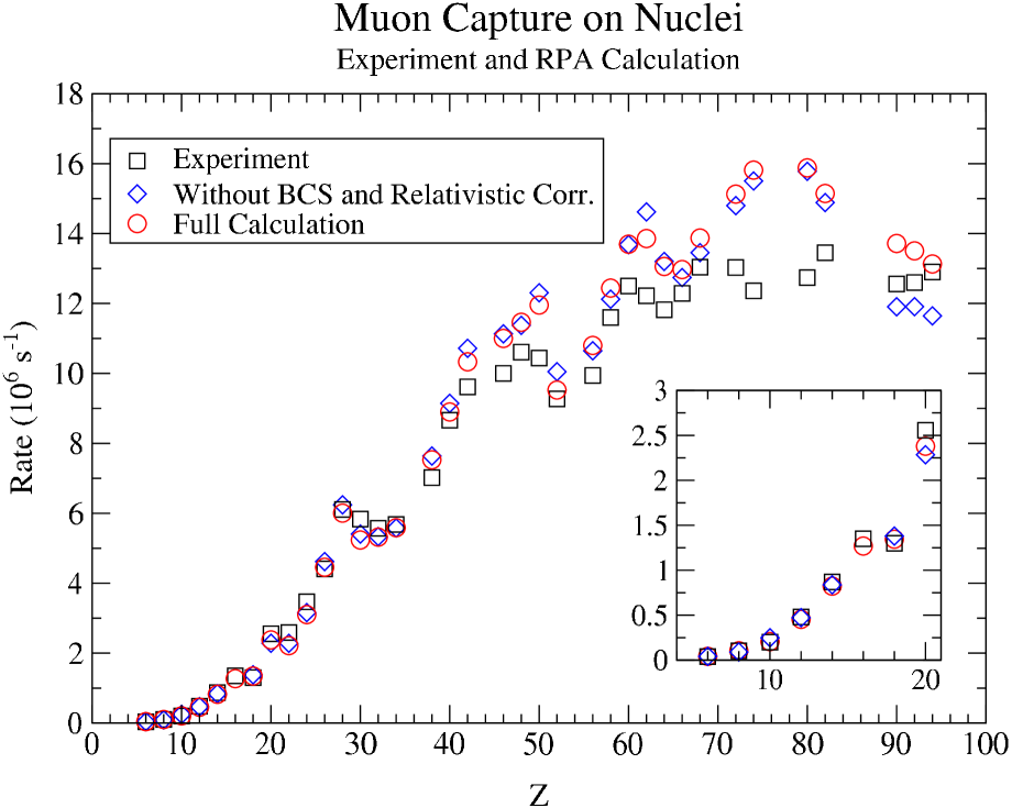
Figure 1: (color online) Comparison between the measured total muon capture rates Measday denoted by squares $\Box$, the calculated rates with all corrections (empty circles $\bigcirc$), and the calculated rates without the BCS and relativistic corrections (diamonds $\Diamond$ ). The insert, in larger scale, shows the same results for light nuclei. When the measurements are for the natural abundance of a given element, the calculation represent the corresponding combination of the individual isotopes.

Our calculated total muon capture rates for all nuclei for which measured values exist are shown in Figure 1. One sees that the overall agreement is quite good. With the exceptions at $Z=74$ and $80$ the calculations reproduce the experimental values to 15% or better. In Figure 2 we provide a ratio plot where the degree of agreement is better seen. In addition, in Table 1 we collect all our calculated capture rates, including the results for individual isotopes.

Nuc	exp	calc	Nuc	exp	calc	Nuc	exp	calc
12C	0.039	0.042	16O	0.103	0.104	18O	0.088	0.089
20Ne	0.204	0.206	24Mg	0.484	0.454	28Si	0.871	0.823
32S	1.352	1.269	40Ar	1.355	1.345	40Ca	2.557	2.379
44Ca	1.793	1.946	48Ca	1.2141	1.455	48Ti	2.590	2.214
natCr	3.472	3.101	50Cr	3.825	3.451	52Cr	3.452	3.085
54Cr	3.057	3.024	56Fe	4.411	4.457	natNi	5.932	6.004
58Ni	6.110	6.230	60Ni	5.560	5.563	62Ni	4.720	4.939
natZn	5.834	5.235	64Zn		5.735	66Zn		4.976
68Zn		4.328	natGe	5.569	5.317	70Ge		5.948
72Ge		5.311	74Ge		4.970	natSe	5.681	5.588
78Se		6.023	80Se		5.485	82Se		5.024
natSr	7.020	7.529	86Sr		8.225	88Sr	6.610	7.445
natZr	8.660	8.897	90Zr		8.974	92Zr		9.254
94Zr		8.317	natMo	9.614	10.33	92Mo		10.80
94Mo		11.01	96Mo		10.04	98Mo		9.153
natPd	10.00	11.00	104Pd		12.71	106Pd		11.44
108Pd		10.44	110Pd		9.607	natCd	10.61	11.46
110Cd		12.58	112Cd		11.51	114Cd		11.21
116Cd		10.44	natSn	10.44	11.95	116Sn		13.08
118Sn		12.35	120Sn		11.64	122Sn		10.82
124Sn		10.15	natTe	9.270	9.523	126Te		10.20
128Te		9.639	130Te		9.043	natBa	9.940	10.80
136Ba		11.45	138Ba		10.73	natCe	11.60	12.44
140Ce		12.38	142Ce		12.95	natNd	12.50	13.70
142Nd		13.67	144Nd		14.12	146Nd		13.15
natSm	12.22	13.86	148Sm		15.01	152Sm		13.23
154Sm		12.08	natGd	11.82	13.06	156Gd		14.15
158Gd		13.06	160Gd		12.03	natDy	12.29	12.97
162Dy		13.45	164Dy		12.54	natEr	13.04	13.87
166Er		14.46	168Er		13.51	170Er		13.22
natHf	13.03	15.13	178Hf		15.44	180Hf		14.89
natW	12.36	15.81	182W		16.37	184W		15.79
186W		15.32	natHg	12.74	15.88	198Hg		17.17
200Hg		16.29	202Hg		15.43	204Hg		14.58
natPb	13.45	15.15	206Pb		15.54	208Pb		14.97
232Th	12.56	13.71	234U	13.79	14.89	236U	13.092	14.17
238U	12.572	13.51	242Pu	12.90	13.13	244Pu	12.403	12.70

Table 1: Calculated rates for natural elements and for the important individual isotopes. All rates are in the form $xx\times 10^{6}$ s^-1. If the natural abundance has more than 90% of a given isotope then the Nuc column gives this particular isotope and the calculation is done for this nucleus only. Whenever a nucleus has the superscript ^nat the calculation is a weighted combination of all isotopes contributing more than 10% to the natural abundance. An empty experiment box means that the given isotope has not been measured. Natural abundance measurements appear in the box next to the most abundant isotope. Experimental data are from Ref. Measday , where the original sources may be found. ¹ is taken from Ref. ca48 , ² is from Ref. Hanscheid and ³ is from Ref. David

In Fig. 1 the total capture rates are also compared with values obtained from calculations where the BCS occupancy and the relativistic corrections are turned off. From this comparison it is clear that these are only small corrections, providing justification for the calculation done in Ref. Kolbe1 ; Kolbe2 ; Kolbe3 . At low $Z$ one especially notices the good reproduction of the distinct dips in the rates above the magic numbers $Z=20$ and $28$. For $Z=50$ the same trends is visible in both calculation and experiment, but the calculations overshoot the experimental values somewhat. Just above $Z=60$, where the $N=82$ closed neutron shell comes into play, we also overestimate the capture rates. This continues into the region with $Z=74$ and $80$, and also, to a lesser extent, to the doubly-magic nucleus ²⁰⁸Pb. One should remember that some of the nuclei above $Z=50$ and below $Z=82$ are deformed and thus have different single-particle structures than the ones given by our spherical mean-field model, thus a perfect agreement should not be expected. The fact that the calculated values are again approaching experiment at Th,U and Pu is likely a consequence of the same dip after the magic shell closure that was seen at lower $Z$ also (these trends were also noted in Ref. Hanscheid , see in particular figure 3 of that reference).

As stated above, we use the unquenched value for the axial-vector coupling constant for all multipole operators, except for the true Gamow-Teller transition. For most of the light- and medium-mass nuclei, $\lambda=1^{-}$ (dipole-like) and $\lambda=2^{+}$ (quadrupole-like) transitions dominate. However, for ²⁰⁸Pb and the heavier nuclei, $\lambda=1^{+}$ transitions contribute significantly to the total capture rate. For these nuclei, the neutron excess is already so large that, in the simple independent particle model, 2 major oscillator shells have to be overcome when changing a proton into a neutron in the muon capture process. Thus, for these excitations the $\lambda=1^{+}$ multipole transition corresponds to a 2$\hbar\omega$ mode and not to a (0 $\hbar\omega$) Gamow-Teller transition; the contribution of the latter to the rate in the heavy nuclei vanishes in our calculations. We have not renormalized the axial-vector coupling constant for such 2 $\hbar\omega$ $1^{+}$ transitions, supported by the good agreement of the the calculated capture rates with the measured results for the heavy nuclei.

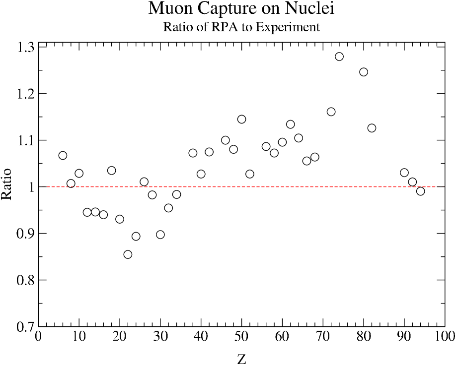
Figure 2: (color online) Ratios of the calculated and measured total muon capture rates vs. the atomic number.

An important test of the ability of a nuclear structure model to reproduce the data is the dependence of the muon capture rate on the number of neutrons for a fixed nuclear charge $Z$. Typically, the rate decreases with increasing $N$ (or $A$) as subsequently more neutron levels are getting blocked. This effect is incorporated into the well-known Primakoff parametrization by its (N-Z) dependence Primakoff . As examples, table 1 include three isotope chains of nuclei (Ca, Cr, and Ni), where total capture rates for individual isotopes have been measured. One sees that the isotope dependence is well reproduced by our calculations. Analogous calculations were performed in Ref . Kolbe4 ; Zinner04 .

IV Conclusion

The present analysis shows that the standard random phase approximation method is capable of describing quite well the total $\mu^{-}$ capture rates for essentially all stable nuclei. The dependence of the capture rate on the isospin, or neutron excess, the so-called Primakoff rule Primakoff , is also fairly well, albeit not perfectly, reproduced. Our calculation even describes the rather subtle effects of shell closures when considering the dependence of the capture rate on $Z$ and/or $A$. There is no indication of the need to apply any quenching to the operators responsible for the muon capture, in particular those involving single-particle transitions from one oscillator shell to another, i.e. other than those involving $0\hbar\omega$ spin and isospin changing operators.

Given the task of describing the capture in a variety of nuclei, including those with high charge $Z$ and nuclei with unfilled shells, it became necessary to consider several effects that have not been typically included previously. One of them is a fully relativistic treatment of the muon bound state, including the effects associated with the ‘small’ $p_{1/2}$ component of its wave function. Another one is the effect of the smearing of the Fermi level (both for protons and neutrons) in nuclei that have nonmagic $Z$ or $N$ numbers. Even though the corresponding corrections are not very large, they contribute noticeably to the overall good agreement between the experimental data and our calculated values.

Our findings then can be used as guidance in the evaluation of a wide variety of semileptonic weak processes on nuclei with similar momentum transfer.

V Acknowledgment

One of us (P.V.) gratefully acknowledges the hospitality at GSI, where part of this work was done.

VI Appendix

In this appendix we give an outline of terms arising from the inclusion of the fully relativistic treatment of the bound muon wave function, i.e., of both the large and small components. The muon wavefunction we use has the form

$$\phi_{jm}=\left(\begin{array}[]{ccccc}ig(r)\Omega_{jlm}(\hat{r})\\ -f(r)\Omega_{jl^{\prime}m}(\hat{r})\end{array}\right)$$ (4)

where the radial functions satisfy the equations

$$\frac{\textrm{d}}{\textrm{d}r}\left(\begin{array}[]{cc}g\\ f\end{array}\right)=\left(\begin{array}[]{cccccc}-\frac{1+\kappa}{r}&E+m_{\mu}-V(r)\\ -E+m_{\mu}+V(r)&-\frac{1-\kappa}{r}\end{array}\right)\left(\begin{array}[]{cc}g\\ f\end{array}\right),$$ (5)

where $g(r),f(r)$ are the large and small components, respectively. Here

$$\kappa=\left\{\begin{array}[]{lll}-(l+1)&,~{}j=l+\frac{1}{2}\\ l&,~{}j=l-\frac{1}{2}\end{array}\right\}$$ (6)

and

$$\Omega_{j,l,m}(\hat{r})=\sum_{m_{l},m_{s}}(l,1/2,j|m_{l},m_{s},m)Y_{l,m_{l}}(\hat{r})\chi_{m_{s}}$$ (7)

These equations are entirely general and can be found in e.g. Ref. greiner1 . Since we assume that the muon is captured from the atomic $1s$ orbit we have $l=0$ and $l^{\prime}=1$. Since $l^{\prime}$ is non-zero, we can no longer just multiply the wavefunction with the irreducible nuclear operators and obtain good total angular momentum. If the positive z-axis is chosen along the direction of the out-going neutrino then its wavefunction becomes

$$\psi=N\left(\begin{array}[]{ccc}\chi_{-}\\ -\chi_{-}\end{array}\right)\exp(i\vec{p}\cdot\vec{x})$$

Here $\chi_{-}$ are the usual spin down Pauli two-spinors and N is a normalization given in greiner1 . This wavefunction makes the neutrino purely left-handed as the standard model prescribes.

The approach used in Wal neglects the small component in the muon wave function and expands the neutrino plane wave in multipoles. As the large component has $l=0$, angular momentum coupling of the muon wave function and the multipole operators is quite straightforward. This is, however, no longer the case if the small component with orbital angular momentum $l=1$ is considered, implying the need for a cumbersome recoupling of angular momenta to regain tensor operators that can be applied in the nuclear Hilbert space. This results in a more complicated expression for the weak Hamiltonian governing muon capture with several new terms. In the notation used in Wal the Hamiltonian with all terms from both components can be written as

$$\mathcal{H}=$$

$$=\frac{2\,{G_{F}\,\cos\theta_{C}\,N^{*}}}{\sqrt{2}}[\sum_{J=0}^{\infty}\sqrt{4\pi}[J](-i)^{J}\{i\delta_{m,-1/2}\left\{\mathcal{M}_{J,0}^{{}^{\prime}}-\mathcal{L}_{J,0}^{{}^{\prime}}\right\}$$

$$+\alpha\left(J-1,J,m+\tfrac{1}{2}\right)\mathcal{T}_{1}\left(J-1,J,m+\tfrac{1}{2}\right)$$

$$+\alpha\left(J+1,J,m+\tfrac{1}{2}\right)\mathcal{T}_{1}\left(J+1,J,m+\tfrac{1}{2}\right)$$

$$-i\beta_{+}(J,J,m)\mathcal{T}_{2}(J,J,m+\tfrac{1}{2})$$

$$-i\beta_{+}(J+1,J,m)\mathcal{T}_{2}(J+1,J,m+\tfrac{1}{2})$$

$$-i\beta_{+}(J+1,J+2,m)\mathcal{T}_{2}(J+1,J+2,m+\tfrac{1}{2})$$

$$-i\beta_{-}(J-1,J-2,m)\mathcal{T}_{3}(J-1,J-2,m+\tfrac{1}{2})$$

$$-i\beta_{-}(J-1,J,m)\mathcal{T}_{3}(J-1,J,m+\tfrac{1}{2})$$

$$-i\beta_{-}(J,J,m)\mathcal{T}_{3}(J,J,m+\tfrac{1}{2})\}$$

$$+\sum_{J=1}^{\infty}\sqrt{4\pi}[J](-i)^{J}\{i\delta_{m,1/2}\left\{\mathcal{J}^{{}^{\prime}el}_{J,1}-\mathcal{J}^{{}^{\prime}mag}_{J,1}\right\}$$

$$-\delta(J-1,J-1,m)\mathcal{T}_{4}(J-1,J-1,m+\tfrac{1}{2})$$

$$-\delta(J-1,J-1,m)\mathcal{T}_{4}(J-1,J-1,m+\tfrac{1}{2})$$

$$-\delta(J,J,m)\mathcal{T}_{4}(J,J,m+\tfrac{1}{2})$$

$$-\delta(J,J+1,m)\mathcal{T}_{4}(J,J+1,m+\tfrac{1}{2})$$

$$-\delta(J+1,J+1,m)\mathcal{T}_{4}(J+1,J+1,m+\tfrac{1}{2})$$

$$+i\eta_{+}(J,J,m)\mathcal{T}_{2}(J,J,m+\tfrac{1}{2})$$

$$+i\eta_{+}(J+1,J,m)\mathcal{T}_{2}(J+1,J,m+\tfrac{1}{2})$$

$$+i\eta_{+}(J+1,J+2,m)\mathcal{T}_{2}(J+1,J+2,m+\tfrac{1}{2})$$

$$-i\eta_{-}(J-1,J,m)\mathcal{T}_{3}(J-1,J,m+\tfrac{1}{2})$$

$$-i\eta_{-}(J,J,m)\mathcal{T}_{3}(J,J,m+\tfrac{1}{2})$$

$$-i\eta_{-}(J-1,J-2,m)\mathcal{T}_{3}(J-1,J-2,m+\tfrac{1}{2})\}]$$

Here we have defined the tensor operators in the nuclear Hilbert space as

$$\mathcal{M}_{J,M}^{{}^{\prime}} = \int\textrm{d}^{3}\vec{x}g(r)Y_{0,0}j_{J}(\kappa x)Y_{J,M}J_{0}$$

$$\mathcal{L}_{J,M}^{{}^{\prime}} = \frac{i}{\kappa}\int\textrm{d}^{3}\vec{x}g(r)Y_{0,0}\nabla\left(j_{J}(\kappa x)Y_{J,M}\right)J_{0}$$

$$\mathcal{J}^{{}^{\prime}mag}_{J,M} = \int\textrm{d}^{3}\vec{x}g(r)Y_{0,0}j_{J}(\kappa x)\vec{\mathcal{Y}}^{M}_{J,J,1}\cdot\vec{J}$$

$$\mathcal{J}^{{}^{\prime}el}_{J,M} = \frac{1}{\kappa}\int\textrm{d}^{3}\vec{x}g(r)Y_{0,0}\nabla\wedge\left(j_{J}(\kappa x)\vec{\mathcal{Y}}^{M}_{J,J,1}\right)\cdot\vec{J}$$

$$\mathcal{T}_{1}(\gamma,\rho,\mu) = \int\textrm{d}^{3}\vec{x}f(r)j_{\rho}(\kappa x)Y_{\gamma,\mu}J_{0}$$

$$\mathcal{T}_{2}(\gamma,\rho,J,\mu) = \int\textrm{d}^{3}\vec{x}f(r)j_{J+1}(\kappa x)\vec{\mathcal{Y}}^{\mu}_{\gamma,\rho,1}\cdot\vec{J}$$

$$\mathcal{T}_{3}(\gamma,\rho,J,\mu) = \int\textrm{d}^{3}\vec{x}f(r)j_{J-1}(\kappa x)\vec{\mathcal{Y}}^{\mu}_{\gamma,\rho,1}\cdot\vec{J}$$

$$\mathcal{T}_{4}(\gamma,\rho,J,\mu) = \int\textrm{d}^{3}\vec{x}f(r)j_{J}(\kappa x)\vec{\mathcal{Y}}^{\mu}_{\gamma,\rho,1}\cdot\vec{J},$$

where $Y$ are the spherical harmonics and $\vec{\mathcal{Y}}$ are the vector harmonics. The first four operators are those involving the large component and are identical with the ones given in Wal . Their tensor character is $(J,M)$. The last four are new operators, i.e. they were ignored in Wal , involving the small component of the muon wavefunction. Their tensor character is $(\gamma,\mu)$. The other indices of the new operators identify terms which originate in the multipole expansion to produce the correct spherical Bessel function in the integrals. The constants appearing in the Hamiltonian above are given by the rather lengthy expressions

$$\alpha(\gamma,\rho,m) = \sqrt{\tfrac{3/2+m}{3}}\sqrt{\tfrac{3}{4\pi}}\frac{[\rho]}{[\gamma]}\left\langle\rho\,1\,\gamma|000\right\rangle\left\langle\rho\,1\,\gamma|0\,m+\tfrac{1}{2}\,m+\tfrac{1}{2}\right\rangle$$

$$\beta_{+}(\gamma,\rho,J,m) = \sqrt{\tfrac{3/2+m}{3}}\sqrt{\tfrac{3}{4\pi}}\sqrt{J+1}[J+1]\left\langle 1\,J+1\,\rho|000\right\rangle$$

$$\times\left\langle 1\,J\,\gamma|m+\tfrac{1}{2}\,0\,m+\tfrac{1}{2}\right\rangle W\left(1\,J+1\,\gamma\,1;\rho\,J\right)$$

$$\beta_{-}(\gamma,\rho,J,m) = \sqrt{\tfrac{3/2+m}{3}}\sqrt{\tfrac{3}{4\pi}}\sqrt{J}[J-1]\left\langle 1\,J-1\,\rho|000\right\rangle$$

$$\times\left\langle 1\,J\,\gamma|m+\tfrac{1}{2}\,0\,m+\tfrac{1}{2}\right\rangle W\left(1\,J-1\,\gamma\,1;\rho\,J\right)$$

$$\delta(\gamma,\rho,J,m) = \sqrt{\tfrac{3/2-m}{3}}\sqrt{\tfrac{3}{4\pi}}[J]^{2}\left\langle 1\,J\,\rho|000\right\rangle$$

$$\times\left\langle 1\,J\,\gamma|m-\tfrac{1}{2}\,1\,m+\tfrac{1}{2}\right\rangle W\left(1\,J\,\gamma\,1;\rho\,J\right)$$

$$\eta_{+}(\gamma,\rho,J,m) = \sqrt{\tfrac{3/2-m}{3}}\sqrt{\tfrac{3}{4\pi}}\sqrt{J}[J+1]\left\langle 1\,J+1\,\rho|000\right\rangle$$

$$\times\left\langle 1\,J\,\gamma|m-\tfrac{1}{2}\,1\,m+\tfrac{1}{2}\right\rangle W\left(1\,J+1\,\gamma\,1;\rho\,J\right)$$

$$\eta_{-}(\gamma,\rho,J,m) = \sqrt{\tfrac{3/2-m}{3}}\sqrt{\tfrac{3}{4\pi}}\sqrt{J+1}[J-1]\left\langle 1\,J-1\,\rho|000\right\rangle$$

$$\times\left\langle 1\,J\,\gamma|m-\tfrac{1}{2}\,1\,m+\tfrac{1}{2}\right\rangle W\left(1\,J-1\,\gamma\,1;\rho\,J\right)$$

Here we have repeatedly used the standard notation $[J]=\sqrt{2J+1}$. All conventions for the Clebsch-Gordan coefficients and W-symbols are those of Edmonds .

In the derivation of the Hamiltonian given above we have used various selection rules for the Clebsch-Gordan coefficients and the W-symbols. Note that some of the terms vanish at low angular momenta, since $\gamma$ and $\rho$ must be positive for any term to contribute. The quantity $m$ in the above expressions corresponds to the spin projection of the muon. Since we consider unpolarized muons we must average over the two values $m=\pm 1/2$.

For completeness we list here the relevant nuclear currents for the muon capture process. These are

$$\hat{\rho}_{V}(\vec{x}) = G_{E}\sum_{j=1}^{A}\tau_{+}(j)\delta^{(3)}(\vec{x}-\vec{x}_{j})$$

$$\hat{\vec{J}}_{V}(\vec{x}) = \frac{G_{E}}{2Mi}\sum_{j=1}^{A}\tau_{+}(j)\left[\delta^{(3)}(\vec{x}-\vec{x}_{j})\overrightarrow{\nabla}_{j}-\overleftarrow{\nabla}_{j}\delta^{(3)}(\vec{x}-\vec{x}_{j})\right]$$

$$+ \frac{G_{M}}{2M}\overrightarrow{\nabla}\wedge\sum_{j=1}^{A}\tau_{+}(j)\,\vec{\sigma}(j)\delta^{(3)}(\vec{x}-\vec{x}_{j})$$

$$\hat{\rho}_{A} = \frac{G_{A}}{2Mi}\sum_{j=1}^{A}\tau_{+}(j)\,\vec{\sigma}\cdot\left[\delta^{(3)}(\vec{x}-\vec{x}_{j})\overrightarrow{\nabla}_{j}-\overleftarrow{\nabla}_{j}\delta^{(3)}(\vec{x}-\vec{x}_{j})\right]$$

$$+ \frac{m_{\mu}G_{P}}{2M}\overrightarrow{\nabla}\cdot\sum_{j=1}^{A}\tau_{+}(j)\,\vec{\sigma}(j)\delta^{(3)}(\vec{x}-\vec{x}_{j})$$

$$\hat{\vec{J}}_{A}(\vec{x}) = G_{A}\sum_{j=1}^{A}\tau_{+}(j)\,\vec{\sigma}(j)\delta^{(3)}(\vec{x}-\vec{x}_{j})$$

here $M$ is the nucleon mass, $G_{E}$ and $G_{M}$ are the Sachs nucleon form factors and $G_{A}$ is the axial form factor. We note that that the usual Fermi and Gamow-Teller transition operators are recovered in the $q\to 0$ limit as the following multipole components (see, e.g. Walecka2 )

$$\mathcal{M}_{0,0} = \frac{1}{\sqrt{4\pi}}G_{V}\sum_{j=1}^{A}\tau_{+}(j)$$

$$\mathcal{L}_{1,M} = \frac{1}{\sqrt{2}}\mathcal{T}_{1,M}^{el}=\frac{i}{\sqrt{12\pi}}G_{A}\sum_{j=1}^{A}\tau_{+}(j)\,\sigma_{1,M}(j)$$

were $G_{V}$ is the $q\to 0$ limit of the vector coupling form factor, which is often denoted by $F_{1}(0)$ in the literature.

To get the final expression for the total rate one must now evaluate the absolute squared matrix element of the Hamiltonian in the initial and final nuclear states and multiply it by the two-body phase space factor given in Wal . It is advantegeous to group together the components with like tensor order to better control the interference of operators arising from the large and small components.

References

- (1) D. F. Measday, Phys. Rep. 354 (2001) 243
- (2) J. D. Walecka in Muon Physics II, edited by V.W. Hughes and C. S. Wu (Academic Press, NY, 1975) p. 113.
- (3) N. C. Mukhopadhyay, Phys. Rep. 30C, 1 (1977).
- (4) T. Suzuki, D. F. Measday, and J. P. Roalsvig, Phys. Rev. C 35, 2212 (1987).
- (5) H. W. Fearing and M. S. Welsh, Phys. Rev. C 46, 2077 (1992).
- (6) N. Auerbach and A. Klein, Nucl. Phys. A422 480 (1984)
- (7) N. Auerbach, N. Van Giai and O. K. Vorov, Phys. Rev. C 56 R2368 (1997)
- (8) H. C. Chiang, E. Oset and P. Fernández de Córdoba, Nucl. Phys. A510 591 (1990)
- (9) J. Nieves, J. E. Amaro, and M. Valverde, Phys. Rev. C 70, 055503 (2000); J. E. Amaro, C. Maieron, J. Nieves, and M. Valverde, Eur.Phys. J A24, 343 (2005).
- (10) E. Kolbe, K. Langanke, and P. Vogel, Phys. Rev. C 50, 2576 (1994).
- (11) E. Kolbe, K. Langanke, and P. Vogel, Phys. Rev. C 62, 055502 (2000).
- (12) N. T. Zinner, K. Langanke, K. Riisager and E. Kolbe, Eur. Phys. J. A17 (2003) 625
- (13) B. H. Wildenthal, Prog. Part. Nucl. Phys. 11, 5 (1984).
- (14) E. Caurier, A. Poves, and A. P. Zuker, Phys. Rev. Lett, 74, 1517 (1995).
- (15) C. D. Goodman and S. B. Bloom, in Spin excitation in nuclei, F. Petrovich et al. eds., (Plenum, NY 1983); G. F. Bertsch and H. Esbensen, Rep. Prog. Phys. 50, 607 (1987); O. Häusser et al., Phys. Rev. C 43, 230 (1991).
- (16) K. Langanke, D.J. Dean, P.B. Radha, Y. Alhassid and S.E. Koonin, Phys. Rev. C52 (1995) 718
- (17) G. Martinez-Pinedo, A. Poves, E. Caurier and A.P. Zuker, Phys. Rev. C53 (1996) R2602
- (18) G. A. Rinker and J. Speth, Nucl. Phys. A306, 306 (1978).
- (19) F. Grümmer and J. Speth, nucl-th/0603052.
- (20) E. Kolbe, K. Langanke, and P. Vogel Nucl. Phys. A652 91 (1999).
- (21) H. Hänscheid et. al., Z. Phys. A - Atomic Nuclei 335 1 (1990)
- (22) A. Fetter and J. D. Walecka Quantum Theory of Many-Particle Systems (McGraw-Hill, San Francisco, 1971).
- (23) A. Bohr and B. Mottelson Nuclear Structure Vol.I (W.A. Benjamin, Inc. 1969), pages 169-171.
- (24) H. O. U. Fynbo et. al., Nucl. Phys. A724 493 (2003).
- (25) P. David et. al. Z. Phys. A - Atomic Nuclei 330 397 (1988)
- (26) H. Primakoff, Rev. Mod. Phys. 31, 802 (1959).
- (27) E. Kolbe, K. Langanke and K. Riisager, Eur. Phys. J. A11 (2001) 25.
- (28) W. Greiner: Relativistic Wave Equations, English Edition, Springer (1996).
- (29) A. R. Edmonds: Angular Momentum in Quantum Mechanics, Princeton University Press (1957).
- (30) J. D. Walecka: Theoretical Nuclear and Subnuclear Physics, 2nd edition, World Scientific, Singapore (2004).