Benchmark calculation of inclusive electromagnetic responses
in the four-body nuclear system

Abstract

Both the no-core shell model and the effective interaction hyperspherical harmonic approaches are applied to the calculation of different response functions to external electromagnetic probes, using the Lorentz integral transform method. The test is performed on the four-body nuclear system, within a simple potential model. The quality of the agreement in the various cases is discussed, together with the perspectives for rigorous ab initio calculations of cross sections of heavier nuclei.

I introduction

A challenging problem in nuclear physics is to calculate nuclear properties microscopically, using realistic nuclear forces. For light systems ($A=2,3$), the Schrödinger equation can be solved with a high degree of accuracy and both ground state properties and reaction cross sections have been calculated Arenhövel and Sanzone (1991); Carlson and Schiavilla (1998); Arenhövel et al. (2005); Marcucci et al. (2005); Skibinski et al. (2005); Golak et al. (2005); Deltuva et al. (2005).

For heavier systems, the Green’s function Monte Carlo (GFMC) method Pieper et al. (2002, 2004) as well as the no-core shell model (NCSM) approach Navrátil et al. (2000a) have been successfully applied for the ab initio description of nuclear properties, using realistic nucleon-nucleon (NN) and three-nucleon forces. GFMC calculations, while more accurate, are limited to masses up to $A=12$, while the NCSM can handle a larger range of masses, up to $A=16$ and beyond Vary et al. (2005); ne (2).

However, for A$>3$ a big obstacle is encountered if one wants to calculate reaction observables involving states in the continuum, because of the enormous difficulties in calculating many-body scattering states.

Such difficulties can be avoided using integral transforms, which reduce the continuum problem to a bound-state-like problem Efros (1985, 1993, 1999), so that only bound state techniques are required. While not all integral transforms are appropriate for a practical use Carlson and Schiavilla (1992); Efros et al. (1993) (the inversion of the transforms is an “ill posed problem” Tikonov and Arsenin (1977)), the integral transform with a Lorentz kernel Efros et al. (1994) appears to be the practical tool for such calculations. In fact, it has allowed the calculation of electromagnetic reaction cross sections beyond break-up thresholds of nuclei from $A=3$ Efros et al. (2005) to A=7 Bacca et al. (2004a). Such calculations have also been possible thanks to the use of the effective interaction hyperspherical harmonic (EIHH) Barnea et al. (2000a, 2003) approach, a very accurate bound state technique, which, similar to the NCSM approach, uses the concept of an effective interaction to speed up the convergence of the basis expansions. In particular, by means of the Lorentz integral transform (LIT) method combined with the EIHH technique, total photoabsorption cross sections of six- Bacca et al. (2002, 2004b) and seven-body nuclei Bacca et al. (2004a) with semirealistic NN potentials have been calculated. In a very recent work Gazit et al. (2006) the ⁴He total photoabsorption cross section could even be calculated with a realistic nuclear force (two- and three-body potential). Moreover, a similar formalism has been recently applied to describe exclusive electromagnetic processes of the four-body nuclear system with a semirealistic potential Quaglioni et al. (2004, 2005); Andreasi et al. (2006).

While the EIHH and NCSM approaches are rather similar, only the latter has made use of realistic interactions in calculations with $A>4$ . Indeed, NCSM has the advantage that one can use an equivalent Slater determinant basis, allowing description of a larger range of masses. Therefore, it is of great interest to investigate the possibility of applying the NCSM to the LIT equations. In fact, if one could obtain reliable results in this way, the possibility to study also reactions on heavier nuclei by means of realistic ab initio approaches would open up.

The purpose of the present work is to investigate the applicability of the NCSM approach to the solutions of the bound-state equations required by the LIT method. The similarities between the EIHH and the NCSM makes the task straightforward, in principle. On the other hand, the practical implementation of the method, especially concerning the problems of convergence, might lead to difficulties.

In the following, we present the results of a test consisting in calculating, within the EIHH and NCSM approaches, the LIT of the four-body response functions to two different excitation operators. Because of the convergence properties, the input interaction is the simple Minnesota (MN) Thomson et al. (1977) potential. Two operators of different nature and range have been chosen, i.e., the isovector dipole and isoscalar quadrupole.

The paper is organized as follows. In Sec. II, the theoretical approaches are discussed, that is the LIT as well as the NCSM and EIHH methods, respectively. Results are presented in Sec. III, while conclusions and perspectives are discussed in Section IV.

II Theoretical overview

II.1 The LIT approach

The inclusive cross sections of reactions induced by perturbative external probes are generally written in terms of the so-called response functions defined as:

$${R(\omega)=\int d\Psi_{f}\left|\left\langle\Psi_{f}\right|\hat{O}\left|\Psi_{0}\right\rangle\right|^{2}\delta(E_{f}-E_{0}-\omega)}\,,$$ (1)

where $\omega$ represents the energy transferred by the probe, and $\hat{O}$ the excitation operator. Wave functions and energies of the ground and final states of the perturbed system are denoted by $\left|\Psi_{0/f}\right>$ and $E_{0/f}$, respectively.

In the LIT method Efros et al. (1994) one obtains $R(\omega)$ after the inversion of an integral transform with a Lorentzian kernel

$$L(\sigma_{R},\sigma_{I})=\int d\omega\frac{R(\omega)}{(\omega-\sigma_{R})^{2}+\sigma_{I}^{2}}=\langle\widetilde{\Psi}|\widetilde{\Psi}\rangle\,.$$ (2)

The state $\widetilde{\Psi}$ is the unique solution of the inhomogeneous “Schrödinger-like” equation

$$(H-E_{0}-\sigma_{R}+i\sigma_{I})|\widetilde{\Psi}\rangle=\hat{O}|{\Psi_{0}}\rangle.$$ (3)

Because of the presence of an imaginary part $\sigma_{I}$ in Eq. (3) and the fact that the right-hand side of this same equation is localized, one has an asymptotic boundary condition similar to a bound state. Thus, one can apply bound-state techniques for its solution, and, in particular, expansions over basis sets of localized functions. In the present paper we solve Eq. (3) using both the NCSM and EIHH methods, which will be briefly described below.

In both cases we evaluate the LIT by calculating the quantity $L(\sigma)=\langle\widetilde{\Psi}|\widetilde{\Psi}\rangle$ directly Marchisio et al. (2003) via the Lanczos algorithm. Hence, one finds that the LIT can be written as a continuous fraction

$$L(\sigma)=\frac{M_{0}}{\sigma_{I}}~{}{\rm Im}\frac{1}{(z-a_{0})-\frac{b_{1}^{2}}{(z-a_{1})-\frac{b_{2}^{2}}{(z-a_{2})-b_{3}^{2}....}}}\,,$$ (4)

in terms of the Lanczos coefficients $a_{n}$ and $b_{n}$, where $\sigma=\sigma_{R}+i\sigma_{I}$ and $z=E_{0}+\sigma$. The quantity

$$M_{0}=\langle\Psi_{0}|\hat{O}^{\dagger}\hat{O}|\Psi_{0}\rangle$$ (5)

is the zero-th moment of the distribution $R(\omega)$ and, therefore, equivalent to the total strength induced by the excitation operator (non-energy weighted sum rule). A parameter-free smooth response function $R(\omega)$ is obtained by inversion of the integral transform of Eq. (2) (for inversion methods see Refs. Efros et al. (1999) and Andreasi et al. (2005)).

Here we would like to note that similar applications have already been used in the past Caurier et al. (1990, 1995) for evaluating response functions by means of shell-model calculations in terms of the so-called “Lanczos response” (LR). In these cases, LR is

$$LR(\omega)=M_{0}\sum_{n=1}^{\mathcal{N}}S_{n}~{}\delta(E_{n}-E_{0}-\omega)\,,$$ (6)

where ${\mathcal{N}}$ is the number of Lanczos iterations, while $E_{n}$ and $S_{n}$ are the eigenvalues and transition strengths obtained with the Lanczos algorithm, respectively. Starting with Eq. (6), one usually replaces the $\delta$ function by a resolution function (Lorentzian or Gaussian) with a width parameter appropriate to the experiment (a typical value is $\sigma_{I}=0.25$ MeV) Haxton et al. (2005), or one evaluates the running integral

$$I(\omega)=\int_{E_{th}}^{\omega}LR(\omega^{\prime})\,d\omega^{\prime}\,,$$ (7)

where $E_{th}$ is the break-up threshold energy of the system. While the LR has the same underlying physical content as $L(\sigma_{R},\sigma_{I})$, since in both approaches one starts from the poles and the residues of the Green’s function, it is evident that the information is processed in a different way. In fact, in the LIT method Eq. (4) is regarded as an integral transform of the response function, which is then recovered via numerical inversion. In this approach, one typically chooses larger values of $\sigma_{I}$ ( $10-20$ MeV), of the order of the strunctures expected in the response function, such that $L(\sigma_{R},\sigma_{I})$ can be calculated with the sufficient numerical precision that allows a stable inversion. After the inversion one recovers a smooth response, which is independent of $\sigma_{I}$ in a large range of values for this parameter.

II.2 The NCSM and the EIHH approaches

The EIHH and NCSM approaches are spectral resolution methods, where one performs an expansion of the Schrödinger wave function in terms of a complete set of basis states: the hyperspherical-harmonics (HH) functions in the EIHH case, and the HO basis functions in the NCSM case. Obviously, due to computational limitations, the basis has to be truncated. The truncated set of states forms the so-called model or $P$-space, and the excluded basis functions build its complementary $Q$-space, such that the sum $P+Q=1$ spans the total Hilbert space. It is well-known that for a given NN interaction the HO and the HH expansions converge rather slowly. In order to accelerate the convergence pattern, both methods make use of an effective interaction introduced by Navrátil et. al. Navrátil and Barrett (1996, 1998), which follows a unitary transformation approach. For the finite $P$-space, the corresponding effective interaction is obtained by means of a unitary transformation Da Providencia and Shakin (1964); Suzuki and Lee (1980); Suzuki (1982); Suzuki and Okamoto (1983). In general, the exact effective interaction for an $A$-body system will have irreducible $A$-body matrix elements, even if the bare interaction is only two-body, and its construction requires the exact solution of the initial problem. Since the solution for the $A$-body problem is the primary goal of the approach, an exact calculation of the effective interaction is not practical, and one has to resort to approximations. Thus, the effective interaction is approximated as a sum of $a$-body effective interaction terms ($a<A)$, derived from the solution of the $a$-body problem. This procedure is called the cluster approximation, and in practice, we use $a=2$ or $3$. The effective Hamiltonian is then obtained by replacing the bare interaction in the $A$-body Hamiltonian by the effective one. However, because of the approximation introduced in order to compute the effective interaction, the resulting eigenvalues of the effective Hamiltonian do not exactly reproduce the values in the full space, the signature being a dependence of the observables on the parameters of the model space. For a given cluster approximation, the eigenenergies converge to the bare ones by increasing the size of the model space. And in the limit $P\longrightarrow 1$ this procedure becomes exact Mintkevich and Barnea (2004). Alternately, one can obtain convergence in a fixed model space by increasing the cluster size, as in this case the approximate effective interaction converges to the exact one.

In the NCSM, one works in an HO basis, and the $P$-space is spanned by states with the total number of HO quanta $N\leq N_{\textrm{max}}$. For the purpose of this paper, we neglect three-body forces and use local interactions, although the non-local interactions do not present an impediment Navrátil et al. (2000b). Therefore, the intrinsic Hamiltonian describing a system of $A$ nucleons is simply

$$H=\frac{1}{A}\sum_{i<j=1}^{A}\frac{(\vec{p}_{i}-\vec{p}_{j})^{2}}{2m}+\sum_{i<j=1}^{A}V(\vec{r}_{i}-\vec{r}_{j})$$ (8)

with $\vec{p}_{i}$ and $\vec{r}_{i}$ being the momentum and the position vectors of the ith particle, respectively; $V$ being the NN potential; and $m$ the nucleon mass. In order to facilitate the use of the convenient HO basis for evaluating the effective interaction, Eq. (8) is modified by adding an HO center-of-mass Hamiltonian $\vec{P}^{2}/(2Am)+Am\Omega^{2}\vec{R}^{2}/2$,

$$\vec{P}=\sum_{i=1}^{A}\vec{p}_{i}\quad{\rm and}\quad\vec{R}=\frac{1}{A}\sum_{i=1}^{A}\vec{r}_{i}\,.$$ (9)

Thus, the $A$-body Hamiltonian takes the form

$$H_{A}^{\Omega} = \sum_{i=1}^{A}\left[\frac{\vec{p}_{i}^{~{}2}}{2m}+\frac{1}{2}m\Omega^{2}\vec{r}_{i}^{~{}2}\right]$$ (10)

$$+ \sum_{i<j=1}^{A}\left[V(\vec{r}_{i}-\vec{r}_{j})-\frac{m\Omega^{2}}{2A}(\vec{r}_{i}-\vec{r}_{j})^{2}\right]\,,$$

where $\Omega$ is the HO parameter. As the NN potential depends on the relative coordinates, the added center-of-mass HO term has no influence on the internal motion in the full space.

In the present NCSM calculations, we use the three-body cluster approximation for the effective interaction. In order to derive it, one solves the three-body problem for the cluster Hamiltonian

$$H_{3}^{\Omega} = \sum_{i=1}^{3}\left[\frac{\vec{p}_{i}^{~{}2}}{2m}+\frac{1}{2}m\Omega^{2}\vec{r}_{i}^{~{}2}\right]$$ (11)

$$+ \sum_{i<j=1}^{3}\left[V(\vec{r}_{i}-\vec{r}_{j})-\frac{m\Omega^{2}}{2A}(\vec{r}_{i}-\vec{r}_{j})^{2}\right]\,\,,$$

and determines the three-body unitary transformation $X^{(3)}$ from the condition that the transformed Hamiltonian

$${\mathcal{H}}^{(3)}=X^{(3)~{}-1}H_{3}^{\Omega}X^{(3)}$$ (12)

preserves the solutions of Eq. (11) in a subspace $P^{(3)}$ of the full three-body Hilbert space. This approximation introduces dependence on the oscillator parameter $\Omega$ so that one has to search for a range of $\Omega$-values that minimizes such a dependence. The effective Hamiltonian for the $A$-body system in the three-body cluster approximation is then defined as

$${\mathcal{H}}_{eff} = \sum_{i=1}^{A}\left[\frac{\vec{p}_{i}^{~{}2}}{2m}+\frac{1}{2}m\Omega^{2}\vec{r}_{i}^{~{}2}\right]$$ (13)

$$+\frac{1}{A-2}\sum_{i<j<k=1}^{A}{\mathcal{V}}^{(3)}_{ijk}\,\,,$$

with

$${\mathcal{V}}^{(3)}={\mathcal{H}}^{(3)}-\sum_{i=1}^{3}\left[\frac{\vec{p}_{i}^{~{}2}}{2m}+\frac{1}{2}m\Omega^{2}\vec{r}_{i}^{~{}2}\right]\,\,.$$ (14)

Note that, because of the decoupling condition

$$Q^{(3)}{\mathcal{H}}^{(3)}P^{(3)}=0\,\,,$$ (15)

the three-body effective interaction is energy-independent. A more detailed description of the derivation of the operator $X^{(3)}$ can be found in Refs. Navrátil et al. (2000b, c); Navrátil and Ormand (2002); Nogga et al. (2005).

In a consistent approach, one should use effective transition operators, derived by means of the same transformation that determines the effective interaction. While the renormalization at the three-cluster level has not been investigated for general operators, studies of the latter in the two-body cluster approximation have shown little effect of the renormalization for long-range observables Stetcu et al. (2005, 2006). Although it is conceivable that a renormalization at the three-body cluster level can show some improvement for long-range operators in smaller model spaces, this task is extremely demanding and not justified since we obtain model space independent results in the largest model spaces used in this work.

The present four-nucleon $P$-space calculations are performed in a properly antisymmetrized translationally invariant HO basis, as described in Navrátil et al. (2000b), where the interested reader can find details on how to compute an one-body translationally invariant operator in such a basis.

In the EIHH method Barnea et al. (2000a, 2003) the calculation is performed with the HH basis and the spaces $P$ and $Q$ are defined by means of the hyperspherical quantum number $K$. Thus, the model space includes all the HH functions with $K\leq K_{\mathrm{max}}$. The intrinsic Hamiltonian in the hyperspherical coordinates is given by

$$H=\frac{1}{2m}\left[-\Delta_{\rho}+\frac{\hat{K}^{2}}{\rho^{2}}\right]+\sum_{i<j=1}^{A}V(\vec{r}_{i}-\vec{r}_{j})\;,$$ (16)

where $\rho$ is the hyperradius and $\Delta_{\rho}$ contains derivatives with respect to $\rho$ only. The grand-angular momentum operator $\hat{K}^{2}$ is a function of the variables of particles $A$ and $(A-1)$ and of $\hat{K}_{A-2}$, the grand angular momentum operator of the residual subsystem Efros (1972). Unlike in the case of NCSM calculation, in this work we use a two-body cluster approximation for EIHH, which already yields an excellent convergence pattern. The starting point for the construction of the effective interaction is a two-body-like Hamiltonian,

$$H_{2}(\rho)=\frac{1}{2m}\frac{\hat{K}^{2}}{\rho^{2}}+V(\vec{r}_{A,A-1})\;,$$ (17)

where $\vec{r}_{A,A-1}$ is the relative coordinate between particles $A$ and $A-1$, but the total hyperspherical kinetic energy is considered. Due to the presence of the hyperradius $\rho$, which is a collective coordinate, the resulting effective interaction produces a sort of “medium correction”. Moreover, since it depends also on the $K_{A-2}$ quantum number of the $A-2$ particle subsystem, it is state dependent. The sum of these leads to a faster rate of convergence. The HH functions are constructed starting from the relative Jacobi coordinates, thus the center of mass motion is removed from the very beginning. The Fermionic basis states are obtained by coupling spin-isospin states, i.e., states that belong to irreducible representations of the permutation group $S_{A}$, with spatial HH states to yield completely antisymmetric basis functions. The basis is constructed by using the powerful algorithms of Barnea and Novoselsky (1997, 1998); Novoselsky and Katriel (1994); Novoselsky and Barnea (1995); Barnea (1999).

III Results

The aim of the present work is to investigate the reliability of the NCSM approach for the description of inclusive response functions via the LIT method, and not to give a realistic prediction of those response functions. Therefore, although applications of the NCSM and the EIHH have already been performed and published using realistic NN forces as well as theoretical three nucleon forces, for the purpose of our comparison it is more convenient to employ the semi-realistic MN Thomson et al. (1977) potential. The advantage of the MN potential is that it consists of Gaussian-type potentials and has a rather soft core, leading to good convergence rate for both the NCSM and the EIHH.

We present results for two operators different in isospin nature and range, giving the leading contribution to low-energy electromagnetic reactions. These are the isovector dipole and the isoscalar quadrupole operators, respectively:

$$\hat{D} = \sqrt{\frac{4\pi}{3}}\sum_{i=1}^{A}\frac{\tau^{z}_{i}}{2}r_{i}Y_{10}(\hat{r}_{i})\,,$$ (18)

$$\hat{Q} = \sqrt{\frac{16\pi}{5}}\sum_{i=1}^{A}\frac{1}{2}r^{2}_{i}Y_{20}(\hat{r}_{i})\,.$$ (19)

The NCSM calculations are also carried out for four different HO frequencies ($\hbar\Omega=12,19,28$ and $40$ MeV), in order to study the dependence of the resulting LIT on this parameter and to provide an estimate for the theoretical uncertainties.

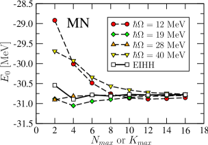
Figure 1: (Color online) ⁴He ground-state energy for the MN potential as a function of the HO excitations allowed in the NCSM model space $N_{max}$ and of the maximal value of the HH grand-angular momentum quantum number $K_{max}$ in the EIHH expansion.

While not the goal of the present calculation, we illustrate the convergence patterns for the ⁴He ground-state energy in Fig. 1. This convergence is important because (i) the ground-state wave function $|\Psi_{0}\rangle$ enters the source term in the LIT equation (2), and (ii) the total strength $M_{0}$ depends entirely on $|\Psi_{0}\rangle$. A good convergence is reached already at $K_{max}=10$ for EIHH, whereas one obtains slower or faster convergence for NCSM, depending on the value of the HO frequency $\Omega$. In particular, one finds a weak dependence on the model space size for $\hbar\Omega=19$ and $28$ MeV. The five best results, which occur for $N_{max}=16$ and $K_{max}=16$, all agree within $0.2\%$. Note that the Coulomb interaction is not included, so that the ⁴He g.s. energy obtained in our calculations differs from previously published results for the MN potential ($-29.96(1)$ MeV Barnea et al. (2000b)).

Table 1: Summary of ⁴He ground-states properties obtained using the MN Thomson et al. (1977) potential model without Coulomb interaction. The evaluation of total strength of the isoscalar quadrupole transition, $M_{0}(\hat{Q})$, for the NCSM does not take into account the $\hbar\Omega=40$ MeV result, which is not yet converged.

	$E_{0}$ [MeV]	$M_{0}(\hat{D})$ [fm2]	$M_{0}(\hat{Q})$ [fm4]
EIHH	$-30.779(1)$	$0.7883(1)$	$8.54(1)\phantom{4}$
NCSM	$-30.80(5)\phantom{1}$	$0.786(6)\phantom{1}$	$8.56(14)$

In Table 1, we compare the ⁴He ground state properties obtained using the MN two-body interaction in both EIHH and NCSM. One finds an excellent agreement for the binding energy, as well as dipole and quadrupole total strengths, which will be discussed in more detail below.

III.1 Dipole response

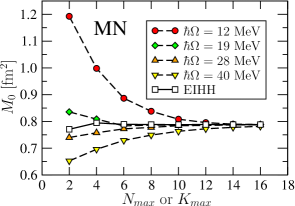
Figure 2: (Color online) ⁴He total dipole strength for the MN potential as a function of the HO excitations allowed in the NCSM model space $N_{max}$ and of the maximal value of the HH grand-angular momentum quantum number $K_{max}$ in the EIHH expansion.

We start the discussion with the results for the isovector dipole transition. In Fig. 2, we compare the total strength $M_{0}$, which enters Eq. (2), for $\hat{O}=\hat{D}$. We evaluate $M_{0}$ for the dipole operator by means of an expansion over basis states with $J^{\pi}T=1^{-}1$. Alternatively, using the non-energy weighted sum rule, one can evaluate $M_{0}$ directly on the ground state as an expectation value of two long-range operators (i.e., the mean square charge radius $\langle r_{ch}^{2}\rangle$ and the mean square proton-proton radius $\langle r_{pp}^{2}\rangle$) Dellafiore and Lipparini (1982),

$${M_{0}=\frac{1}{3}\left[Z^{2}\left<r_{ch}^{2}\right>-\frac{Z(Z-1)}{2}\left<r_{pp}^{2}\right>\right]\,.}$$ (20)

As expected, the sum rule is satisfied for each model space. The rate of convergence of the total strength depends upon the HO frequency, as it does for the g.s. energy and other observables, and the least dependence on the model space is obtained again for $\hbar\Omega=19$ and $28$ MeV. Also, the best EIHH and NCSM results ($N_{max}$ or $K_{max}=16$) agree within $0.1\%$ for $\hbar\Omega=12,19$ and $28$ MeV, whereas one finds a larger deviation ($0.8\%$) for $\hbar\Omega=40$ MeV, not yet completely convergent. The origin of this behavior is related to the fall-off of the wave function for the HO potential well. As the HO potential well becomes steeper and steeper, the wave functions in a fixed model space go faster to zero; as a consequence, one finds smaller root-mean square radii for the ⁴He g.s., and the expectation value of a long-range operator, like the isovector dipole, is more poorly represented. In principle, we could improve the convergence of $M_{0}$ for $\hbar\Omega=40$ MeV by calculating the expectation value of $D^{\dagger}D$ directly on the ground state up to $N_{max}=20$. We would like to point out that, despite this, the discrepancy never exceeds the $1\%$.

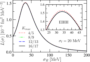
Figure 3: (Color online) The LIT [see Eq. (2)] for the isovector dipole transition as a function of $\sigma_{R}$ for $\sigma_{I}=20$ MeV: convergence of the EIHH calculation with respect to the maximal value of the HH grand-angular momentum quantum numbers $K_{max}$/$(K_{max}+1)$ in the EIHH expansions.

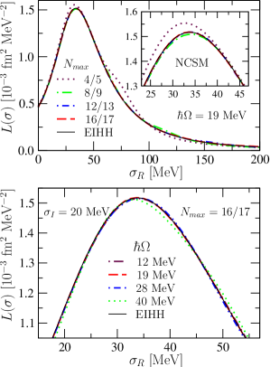
Figure 4: (Color online) The LIT [see Eq. (2)] for the isovector dipole transition as a function of $\sigma_{R}$ at $\sigma_{I}=20$ MeV: convergence with respect to the HO excitations allowed in the NCSM model space for $\Omega=19$ MeV (upper panel), and dependence on the HO frequency $\Omega$ of the best ($N_{max}=16/17$) NCSM results (lower panel). The solid line represents the EIHH result for $K_{max}=16/17$.

The overall convergence behavior of the LIT [see Eq. (2)] is influenced by the convergence of its two components: (i) the total strength $M_{0}$, which was discussed earlier; (ii) the residual continued fraction of Lanczos coefficients. While the first is governed by the convergence of the ground state (non-energy weighted sum rule), the results for the continued fraction have a further dependence on the $J^{\pi}T=1^{-}1$ model space. For this reason, the convergence pattern of the LIT has to be studied as a function of the model space for the ground state as well as for the LIT state $|\widetilde{\Psi}\rangle$. Due to the parity difference of the two states, the values of $K_{max}$ and $N_{max}$ chosen for the model spaces are even for the ground state and odd for $J^{\pi}=1^{-}1$ state, respectively.

Figure 3 shows that the convergence of the LIT for EIHH is fast and accurate over the entire range of $\sigma_{R}$. The same plot for the NCSM results at $\hbar\Omega=19$ MeV, presented in the upper panel of Fig. 3, reveals a slower convergence rate. In particular, we notice that, unlike for the EIHH, the high $\sigma_{R}$ tails of the NCSM results show oscillations and a satisfactory quenching of such oscillations is obtained only for the biggest model space ($N_{max}=16/17$). Furthermore, one finds a stronger dependence on the model-space size, even in the peak region (see the insets of Figs. 3 and 4).

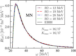
Figure 5: (Color online) The NCSM ($N_{max}=16/17$) inclusive response to the isovector dipole transition [see Eq. (1)] as a function of $\omega$ for four different values of the HO parameter $\Omega$: comparison with the EIHH ($K_{max}=16/17$) result.

The influence of the HO frequency on the LIT is shown in the lower panel of Fig. 4. In a given model space, for smaller HO frequencies one obtains a better sampling of the complex-energy continuum, and therefore a more accurate convergence of the LIT, especially in the low-$\sigma_{R}$ region; on the other hand, faster convergence is achieved when the HO length parameter is chosen close to the size of the state to be described, and, therefore, larger $\hbar\Omega$ values are preferrable for describing the ground state. As a consequence, in the particular case of the ⁴He nucleus, frequencies in the range $12{\rm MeV}\leq\hbar\Omega\leq 28{\rm MeV}$ represent a good compromise, as shown in Fig 4 (lower panel). Among the four frequencies adopted to evaluate the LIT with the NCSM, $\hbar\Omega=19$ MeV leads to the smoothest convergence pattern and to the best agreement with the EIHH curve, which appears as a solid line in Fig. 4.

The different behavior of the two methods with respect to the size of the $P$-space used in the calculation is related both to the differences in the shape and asymptotic behavior of the HO and HH base states Fomin and Efros (1981); Barnea et al. (1999), and, more importantly, to the actual number of states, included in the expansion. We would like to point out that, due to the extra flexibility of the HH basis in the hyperradial part of the expansion, for the same value of $N_{max}$ and $K_{max}$, the number of totally antisymmetric basis states in the two approaches is significantly different. For example, in the model space defined by $N_{max}=16$, one has $2,775$ four-body states for a NCSM calculation, while for $K_{max}=16$, the total number of four-body states in a EIHH calculation is $10,890$. Further details on the connection between the number of basis states in the two approaches can be found in Refs. Barnea et al. (2000a) and Barnea and Mandelzweig (1992).

Figure 5 shows the EIHH and NCSM results for the inclusive response to the isovector dipole excitation obtained by inverting the LIT’s of Figs. 3 and 4. (Note that the same results for the response are obtained by inverting the LIT for $\sigma_{I}=10$ and $15$ MeV.) The HO frequency value of $\hbar\Omega=19$ MeV leads to the best agreement with the EIHH response. Indeed, the discrepancy between the two numerical results does not exceed $5\%$ in the energy intervals immediately close to the disintegration threshold as well as in the dipole resonance peak region. While the resonant peak is equally well described for $\hbar\Omega=12$ and $28$ MeV, these HO frequencies yield a larger discrepancy (at most $10\%$ and $15\%$, respectively) within $3$ MeV from threshold. As expected from previous observations, poorest agreement is found for $\hbar\Omega=40$ MeV, although mainly in the low-energy part of the response. In the range $60$ MeV$\leq\omega\leq 80$ MeV all four NCSM responses agree within the $7\%$ or better of the EIHH result.

III.2 Quadrupole response

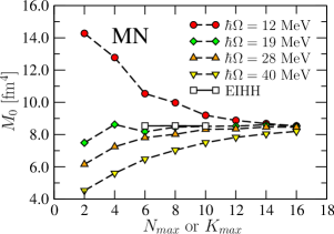
Figure 6: (Color online) ⁴He total quadrupole strength for the MN potential as a function of the HO excitations allowed in the NCSM model space and of the maximal value of the HH grand-angular momentum quantum number $K_{max}$ in the EIHH expansion.

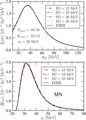
Figure 7: (Color online) The dependence on the HO frequency $\Omega$ of (upper panel) the LIT for $\sigma_{I}=20$ MeV, and (lower panel) the inclusive response for the isoscalar quadrupole transition. Note that $N_{max}=16/16$ is not a complete model space (see text for details). The solid lines represent the EIHH results for $K_{max}=10/12$.

We present now the results for the isoscalar quadrupole transition. As expected, the total strength $M_{0}$ for the isoscalar quadrupole, shown in Fig. 6, presents a slower convergence rate than the same quantity for the dipole operator. The greatest sensitivity to the model-space size is obtained again for $\hbar\Omega=40$ MeV. The calculation of the total strength for the quadrupole transition employs an expansion over an intermediate set of basis states with $J^{\pi}T=2^{+}0$. In particular, for the NCSM values in the largest model space ($N_{max}=16/16$), we omit the contribution of the transitions to the $J^{\pi}T=2^{+}0$ states with $N_{max}=18$, as a full calculation in this case would be out of reach. In principle, one could evaluate the loss of strength induced by such an approximation (introduced due to computational limitations), using the non-energy weighted sum rule and calculating the expectation value of the operator $\hat{Q}^{\dagger}\hat{Q}$ directly on the ground state, as was done for the dipole response. However, the form of this operator makes the calculation technically difficult. As for the dipole transition, the EIHH calculation shows a fast convergence. The agreement with the NCSM results is within the 1% for $\hbar\Omega=12,19$ and $28$ MeV, while $\hbar\Omega=40$ MeV, for which the convergence is not completely reached, shows a 5% discrepancy. Hence, we can assume that the transitions to $N_{max}=18$ can be neglected.

The comparison of the LIT’s in the biggest model space ($N_{max}=16/16$, $K_{max}=10/12$) for the EIHH and the four different NCSM calculations is presented in the upper panel of Fig. 7. All the curves, excluding the result for $\hbar\Omega=40$ MeV, still far from convergence, show a good agreement, and the corresponding inversions are compared in the lower panel of Fig. 7. The discrepancies in the response functions do not exceed the 10% in the range $25~{}{\rm MeV}\leq\omega\leq 60~{}{\rm MeV}$, where the curve shows a resonant behavior. More delicate are the regions close to threshold and high-energy tail, where the response is small and the inversion procedure is more sensitive to the numerical error present in the LIT. One finds the best agreement for $\hbar\Omega=12$ MeV.

IV Conclusions and outlook

We have presented the results of an ab initio calculation of the ⁴He response functions to the isovector dipole and isoscalar quadrupole excitations, obtained by means of the LIT method, within both the NCSM and the EIHH approaches. As NN interaction, we have used the semirealistic MN potential model. The aim has been to investigate the reliability of the NCSM to the description of inclusive response functions via the the integral transform method with a Lorentzian kernel. The chosen transitions have allowed us to perform the test for two operators different in isospin nature and range. In both cases our model study has shown that the NCSM can be successfully applied to the solution of the bound-state-like equations required by the LIT methods. However, due to differences in the asymptotics of the wave functions and in the strength distribution in the continuum achieved with the HO and HH expansions, the practical implementation of the method, especially concerning the problems of convergence, might lead to difficulties. In particular, to ensure a small numerical uncertainty in the response function, obtained by numerical inversion Efros et al. (1999); Andreasi et al. (2005), one has to achieve a very good accuracy in the calculation of the LIT. Consequently, it is necessary to find a range of HO frequencies, for which both the ground and the excited states of the system present good convergence properties. The actual choice of $\hbar\Omega$ depends on both the nucleus under consideration and the range of the transition operator. For ⁴He we find that frequencies in the range $12~{}{\rm MeV}\leq\hbar\Omega\leq 28~{}{\rm MeV}$ have the demanded characteristics for both the isovector dipole and isoscalar quadrupole excitations.

Our main conclusion is that, in this benchmarking calculation with a semirealistic NN interaction, the NCSM is able to reach the level of precision required for the description of continuum responses via the LIT method and to obtain equivalent results as those found with the EIHH method. Because of the ability of NCSM to handle heavier mass nuclei than the EIHH, the present result opens the door for possible LIT investigations of heavier nuclei. However, the large model spaces needed in the NCSM calculations in order to achieve the necessary accuracy will require considerable thought and effort, but may be assisted by the use of effective field-theory two- and three-body interactions, which should be softer.

Since LIT requires a good description of the ground-state wave function, and, at the same time, a fine enough discretization of the complex-energy continuum, one could use a mixed-mode approach in the spirit of Ref. Gueorguiev et al. (2002). Thus, one could use basis states with a frequency that ensures fast convergence for the ground state, adding also basis states of smaller frequencies, which would allow a better discretization of the complex-energy continuum at low energies, and basis states corresponding to larger frequencies for a better description of the response at higher energies. This approach would require, however, a more involved numerical technique which can be adapted for our no-core calculations in a Jacobi basis. Moreover, such a method is not immediately applicable to Slater determinant basis codes, which are much more efficient for calculations in heavier nuclei, because of the more delicate treatment of the center-of-mass motion required in such a case. While such an approximation is under consideration, we leave its possible implementation for future work.