The order, shape and critical point for the quark-gluon plasma phase transition

Abstract

The order, shape and critical point for the phase transition between the hadronic matter and quark-gluon plasma are considered in a thermodynamical consistent approach. The hadronic phase is taken as Van der Waals gas of all the known hadronic mass spectrum particles $m_{H}\leq 2.0$ GeV as well as Hagedorn bubbles which correspond hadronic states with mass spectrum $m_{H}>2.0$ GeV. The density of states for Hagedorn bubbles is derived by calculating the microcanonical ensemble for a bag of quarks and gluons with specific internal color-flavor symmetry. The mixed-grand and microcanonical ensembles are derived for massless and massive flavors. We find Hagedorn bubbles are strongly suppressed in the dilute hadronic matter and they appear just below the line of the phase transition. The order of the phase transition depends on Hagedorn bubble’s internal color-flavor structure and the volume fluctuation as well. On the other hand, the highly compressed hadronic matter undergoes a smooth phase transition from the gas of known mass spectrum hadrons to another one dominated by Hagedorn bubbles with specific internal color-flavor structure before the phase transition to quark-gluon plasma takes place at last. The phase transition is found a first order for the intermediate and large chemical potentials. The existence of the tri-critical point depends on the modification of the bubble’s internal structure specified by a phenomenological parameter $\gamma\propto\mu_{B}$ in the medium.

I Introduction

The thermodynamical description of the strongly interacting hadronic matter gas can be approximated by a free gas with a modified level density. This new level density is given by the statistical bootstrap equation and its solution is the asymptotic mass spectral function for hadronic fireballs with mass exceeding 2 GeV. A solution to this equation exists only for some range of parameters Hagedorn (1965). However, the bootstrap model with internal symmetry Redlich and Turko (1980) of the fireball provides subsidiary variables and allows for new types of the phase transition Antoniou et al. (12005); Kapoyannis et al. (1998a, b). The hadronic fireballs are bags of confined quark and gluon components and stand for highly excited exotic hadrons; we denote them in the following as Hagedorn bubbles. Furthermore, these Hagedorn states have received much attention to understand the phase transition in terms of the AdS black hole duality Aharony et al. (2004, 2005) and the gauge field Dumitru et al. (2004, 2005).

Quarks and gluons are confined due to color confinement while the low-lying hadronic mass spectrum is generated by the broken chiral symmetry. The hadron’s constituent quarks are massive even for light flavors. However, the constituent quark mass decreases slowly with respect to temperature and then drops quickly to its current mass at the critical temperature. It also decreases with respect to the baryonic chemical potential. The decreasing of u,d- quark’s constituent mass near the phase transition is not fully understood. Furthermore, the internal color symmetry of the bound state remains to be that of a color singlet even for finite temperature and chemical potential due to color confinement. When the temperature reaches the critical one, color is expected to be liberated and chiral symmetry is restored. QCD predicts a phase transition from the hadronic gas phase to a deconfined quark-gluon plasma phase. The order of the phase transition for hot and dense hadronic matter, however, remains unclear whether it is first, second, higher order, or just a rapid but smooth crossover. The internal structure of the hadronic quark and gluon bag remains in a total color singlet state. In more realistic calculations, the internal structure is imposed in the partition function for Hagedorn bubbles Muller and Rafelski (1982). In the standard MIT bag model, the quarks and gluons are confined within a sharp surface, which represent a boundary between different media: a perturbative vacuum inside the bag where the quarks and gluon can be approximated as an ideal gas, due to the asymptotic freedom of QCD, and a nonperturbative vacuum outside the bag where free quarks do not exist due to confinement.

The hadronic phase consists of the whole hadronic mass spectrum including resonances of all the known particles. Hard core repulsive forces can be represented by an excluded volume. Effects from strong interactions are included by adding a free gas of Hagedorn bubbles which are bags of constituent quarks and gluons with specific internal color-flavor structure. Despite of complexity of the internal color-flavor structure, Hagedorn bubbles remain to be in an overall color singlet state. With increasing baryonic density at low temperature, the bubble size grows but retains its own internal color symmetry. This means that volume fluctuation is expected to be suppressed whenever the bags start to overlap with each other for a large chemical potential. When the temperature increases, the surface is smeared out until finally the bubbles dissociate at the critical temperature. Therefore, it is expected the bubble volume fluctuation increases when the temperature increases.

The (grand) canonical ensemble and its Laplace transform to the micro-canonical ensemble for gluonic bags or glueballs was derived by Kapusta Kapusta (1981) without imposing any color constraint. The internal symmetry constraint was originally introduced for the statistical bootstrap model Redlich and Turko (1980). The bootstrap density of states can be derived from the MIT bag model. In the hadronic phase, the highly excited fireballs derived from the bootstrap equation are Hagedorn bubbles (e.g. gas of bags) of confined quarks and gluons in a color singlet state or colorless charge.

The colorless bubble is usually less restricted than the color singlet state. The color charges are set to zero for the colorless state $n_{\mbox{C}i}=\frac{\partial\Omega_{V}}{\partial i\phi_{\mbox{C}i}}=0$, where $\Omega_{V}$ is the bubble grand potential density and $\phi_{\mbox{C}i}$ are the color parameters in the $SU(N_{c})$ representation. In the less strict constraint the color charges $n_{3}$ and $n_{8}$ are set to zero for the gas of bags instead for any individual bag. The asymptotic approximation for the colorless charge is given by $i\phi_{\mbox{C}i}\rightarrow 0$. Hence the colorless bubble is usually approximated to an ideal gas of quarks and gluons with the conserved color charge $i\phi_{\mbox{C}i}\rightarrow\mu_{\mbox{C}i}/T\sim 0$. On the other hand, the color singlet state is the ground symmetry projection for the $SU(N_{c})$ representation. This resemblance between the color singlet and colorless states requires to search for the color saddle points around $\frac{\phi_{\mbox{C}i}}{\pi}\ll 1$ and to avoid the Cauchy integral which is used extensively in the literature in the large $N_{c}$ limit Gross and Witten (1980).

Gorenstein et. al. Gorenstein et al. (1984, 1982, 1983) have studied the gas of bags which correspond Hagedorn states using the isobaric partition function. They measured the volume fluctuation for the hadronic bags by differentiating the micro-canonical ensemble with respect to the fixed bag volume. The micro-canonical ensemble only measures the mass spectral density and does not include the actual volume fluctuation. The real deconfinement phase transition from the hadronic phase to the color quark and gluon bags did not take place in their approach. The authors of Refs. Gorenstein et al. (1984, 1982, 1983) argue that the phase transition is only possible when Hagedorn bubble expands rapidly to form a big color singlet quark-gluon droplet which occupies the entire space. Recently, they have pointed out that the phenomenology of Hagedorn bubble internal symmetry decides the order of the phase transition for low chemical potential and high temperature Gorenstein et al. (2005). Unfortunately their model fails to predict the phase transition for deconfined quark-gluon plasma but instead a new phase of matter appears which retains the internal symmetry of Hagedorn bubble. They also were unable to explain how the order of the phase transition can be switched from a lower one to higher ones. On the other hand, Auberson et. al. Auberson et al. (1986a) have shown that the phase transition to a deconfined QGP is granted when asymptotic volume fluctuation is taken into account correctly. They emphasize that the micro-canonical ensemble measures only the mass spectrum for a specific bag volume, which is not the actual volume fluctuation for the quark and gluon bag. Furthermore, it is well known that the bootstrap density of state can be obtained when the bag volume is fixed to $v=m/4B$. Auberson et. al. Auberson et al. (1986a) have approximated the volume fluctuation by allowing the bag mass variation with respect to the volume up to the second order in the distribution function. Furthermore, they have argued that by relaxing the internal symmetry constraint for the color singlet state the resultant Gaussian-like volume fluctuation leads to a second order deconfined phase transition. Hence, the color singlet constraint imposed on the bag states is not a critical for the phase transition’s existence. Therefore, the appearance of the deconfined phase transition depends essentially on the bubbles’ volume fluctuations beside their internal structure constraints.

Hagedorn bubbles likely appear for the highly compressed hadronic matter. These Hagedorn bubbles coalesce and form hadronic bubbles foam. This state of matter is not a deconfined phase. However, when this highly compressed foam of Hagedorn bubbles is heated, the hadronic foam undergoes a smooth phase transition and forms a big quark-gluon droplet as the surfaces between bubbles dissolve. At low baryonic density and high temperature, the situation is rather different. The formation of Hagedorn bubbles is unlikely to take place in the hadronic phase and whenever they appear because of the thermal fluctuations and they shall be suppressed by the gas pressure of the external hadronic mass spectrum particles in particular those relatively large Hagedorn bubbles. However, when the temperature reaches the critical value, some explosive hadronic bubbles can appear in the system. Whenever the internal pressure of the thermal fluctuated bubble approaches the external one for the gas of the mass spectrum hadrons, these bubbles grow up and expand rapidly forming the deconfined quark-gluon plasma at last.

The outline of the present paper is as follows. In section II, we derive the canonical ensemble for a quark-gluon bubble with internal color-flavor symmetry with massless and massive flavors. The micro-canonical ensemble is derived from the inverse Laplace transform of the grand-canonical one. In section III, we review the isobaric partition function for the gas of bags with excluded volume. We also summarize the conditions of the phase transition in the isobaric partition function construction for the gas of bags. The small excluded volume for baryons and mesons and large excluded volume for Hagedorn bubbles are introduced in section IV. In section V, we present two models for the volume fluctuation in the isobaric partition function. The order and shape of the phase transition to quark-gluon plasma is analyzed in section VI. Then we present our scenario for the phase transition to quark-gluon droplets or plasma for low and intermediate chemical potentials and to foam of Hagedorn bubbles for large baryonic chemical potentials in section VII. Finally, we give our conclusions in section VIII.

II Grand canonical and microcanonical ensembles for a quark and gluon bubble with internal color-flavor symmetry and massive constituent quarks

In this section, we derive the (mixed-) grand microcanonical ensemble for an ideal gas of quarks and gluons which are confined inside a bubble of specific size which carry specific internal color-flavor symmetry. Contrary to previous calculations Auberson et al. (1986b); Gorenstein et al. (1983); Elze et al. (1983, 1984); Lang et al. (1981); Skagerstam (1984); Tounsi et al. (1998), we perform the derivation also for massive constituent quarks. The microcanonical ensemble is calculated by taking the inverse Laplace transform of the mixed grand canonical ensemble. The volume fluctuation is introduced by going beyond the standard MIT bag model description with a sharp surface to bag models with an extended surface and bubbles with volume fluctuations. We assume that the volume fluctuation is measured by the bubble volume distribution function. In this context, we propose that the volume distribution function is determined by a smeared volume and mass relation relaxing the corresponding constraint of the the standard bag model.

II.1 (Mixed-) Grand canonical ensemble

The grand canonical ensemble for an ideal gas of quarks and gluons confined in a specific volume can be calculated by Kapusta (1981, 1982); Auberson et al. (1986b); Gorenstein et al. (1983); Elze et al. (1983, 1984); Lang et al. (1981); Skagerstam (1984); Tounsi et al. (1998)

$${\cal Z}_{V}(\beta,\vartheta) = \mbox{Tr}\hat{\cal P}_{a}e^{-\beta\hat{H}+i\vartheta\hat{N}},$$ (1)

where $\hat{H}$ is the Hamiltonian of the physical system, $\hat{N}$ is the conserved quantum number operator. The imaginary chemical potential $\vartheta$ can be written in term of fugacity $i\vartheta=\log\lambda$ in the mixed grand canonical ensemble where $\lambda=e^{\mu/T}$. The operator $\hat{\cal P}_{a}$ selects those configurations that are allowed by specific constraints due to the internal symmetries Redlich and Turko (1980); Turko (1981); Auberson et al. (1986b); Gorenstein et al. (1983); Elze et al. (1983) of the system

$$\hat{\cal P}_{a}\equiv\hat{\cal P}_{j}\cdot\hat{\cal P}_{\hat{\vec{P}}=0}\cdot\hat{\cal P}_{\vartheta}\cdots,$$ (2)

where $\hat{\cal P}_{j}$ project the color component such as the color singlet state, $\hat{\cal P}_{\hat{\vec{P}}=0}$ transforms the system into the center of mass frame Kapusta (1982) while $\hat{\cal P}_{\vartheta}$ conserves the total number of particles in the fireball. In the present model, we consider a quark-gluon gas with specific internal symmetry by introducing three projectors. The color projector of the subspace of all states that transform under the representation $j$ of the irreducible representation ${\cal G}(g)$ of a compact Lie group $\mbox{SU}(N_{c})$ reads

$$\hat{\cal P}_{j}=d_{j}\int_{SU({N_{c}})}d\mu(g)\chi_{j}(g),$$ (3)

where

$$d\mu(g)=\frac{1}{{N_{c}}!}\left(\frac{1}{2\pi}\right)^{N_{c}}\prod_{n>m}^{N_{c}}\left(2\sin\left(\frac{\theta_{n}-\theta_{m}}{2}\right)\right)^{2}2\pi\delta\left(\sum^{N_{c}}_{n=1}\theta_{n}\right)d\theta_{1}d\theta_{2}\cdots d\theta_{N_{c}},$$ (4)

is the normalized Haar measure on ${\cal G}(g)$. However, for small color angles $\frac{\theta_{n}}{\pi}\ll 1$, the Haar measure can be approximated by

$$d\mu(g)\approx\frac{1}{N!}\left(\frac{1}{2\pi}\right)^{N_{c}}\left(\prod^{N_{c}}_{n>m}\left(\theta_{n}-\theta_{m}\right)^{2}\right)2\pi\delta\left(\sum^{N_{c}}_{n=1}\theta_{n}\right)d\theta_{1}d\theta_{2}\cdots d\theta_{N_{c}}.$$ (5)

It is also convenience to introduce the set $\phi_{i}$ where $\theta_{i}=\phi_{i}$ for $i=1,\cdots,N_{c}-1$ and $\phi_{N_{c}}=-\sum^{N_{c}-1}_{k=1}\phi_{k}$. We have introduced the set $\{\phi_{i}\},i=1,\dots,N_{c}-1$ for the group representation $SU(N_{c})$ while the set $\{\theta_{i}\},i=1,\dots,N_{c}$ is introduced for the group $U(N_{c})$. In context of set $\phi_{i}$ the Haar measure reads

$$d\mu(g)\approx\frac{1}{N_{c}!}\left(\frac{1}{2\pi}\right)^{N_{c}-1}\left(\prod^{N_{c}}_{n>m}\left(\phi_{n}-\phi_{m}\right)^{2}\right)d\phi_{1}d\phi_{2}\cdots d\phi_{N_{c}-1}.$$ (6)

The quantities $d_{j}$ and $\chi_{j}(g)$ are the dimension and the orthonormal basis $j$ of the representation, respectively. The basis $\chi_{\mbox{singlet}}(g)=1$ with $d_{j}=1$ projects on the color singlet state for the quark-gluon bubble. The zero momentum projector for the system enclosed in a volume ${\left<V\right>}$ reads

$$\hat{\cal P}_{\hat{\vec{P}}=0} = \int_{\left<V\right>}\frac{d^{3}R}{\left<V\right>}e^{i\vec{P}_{G}\cdot\vec{R}}e^{i\vec{P}_{Q}\cdot\vec{R}}e^{i\vec{P}_{\overline{Q}}\cdot\vec{R}},$$ (7)

$$= \int_{{\left<V\right>}/\beta^{3}}\frac{d^{3}r}{{\left<V\right>}/\beta^{3}}e^{i\beta\vec{P}_{G}\cdot\vec{r}}e^{i\beta\vec{P}_{Q}\cdot\vec{r}}e^{i\beta\vec{P}_{\overline{Q}}\cdot\vec{r}},$$

where we have replaced $R=\beta r$. This constraint means that we are working in the center of mass frame of the quark and gluon bubble Kapusta (1982). However this projection correlates the quarks and gluons in a specific momentum configuration. This projection constrains the momenta of constituent quarks and gluon in a specific alignment

$$\sum_{i}\vec{p}_{Qi}+\sum_{j}\vec{p}_{\overline{Q}_{j}}+\sum_{k}\vec{p}_{Gk}=0~{}\rightarrow\int_{\left<V\right>}\frac{d^{3}R}{\left<V\right>}e^{i\left[\vec{P}_{G}\cdot\vec{R}+\vec{P}_{Q}\cdot\vec{R}+\vec{P}_{\overline{Q}}\cdot\vec{R}\right]}.$$ (8)

The thermal bath breaks the Lorenz invariance. Therefore, it is expected that the high temperature breaks badly this projection. Breaking the momentum projection modifies the density of states significantly. We retain this projection in our calculations although it is not a realistic one for the dense and hot medium as far it is related in somehow to flavor correlations. The argument of breaking this symmetry smoothly with temperature is the beneath of the introduction of the phenomenological modification of the density of states. We relate this modification to the color-flavor correlation. However, in order to soften the equation of state for cold quark matter it is also possible to impose a higher order constraint in the momentum space such as

$$\sum_{i}\vec{p}_{Qi}=\sum_{j}\vec{p}_{\overline{Q}_{j}}=\sum_{k}\vec{p}_{Gk}=0~{}\rightarrow\int_{\left<V\right>}\frac{d^{3}R_{G}}{\left<V\right>}\int_{\left<V\right>}\frac{d^{3}R_{Q}}{\left<V\right>}\int_{\left<V\right>}\frac{d^{3}R_{\overline{Q}}}{\left<V\right>}e^{i\left[\vec{P}_{G}\cdot\vec{R}_{G}+\vec{P}_{Q}\cdot\vec{R}_{Q}+\vec{P}_{\overline{Q}}\cdot\vec{R}_{\overline{Q}}\right]}.$$ (9)

On the other hand, for the crystallized quark matter, it is convenience to introduce the orthogonal representation $O(N)$ for the rotational symmetries in order to soften the equation of state. These aspects is not considered in the present work.

The conserved charge, such as the baryon number $N_{B}$, is guaranteed by

$$\hat{\cal P}_{\vartheta}=\int^{\pi}_{-\pi}\frac{d\vartheta}{2\pi}e^{i\vartheta\left[(N_{Q}-N_{\overline{Q}})-N_{B}\right]}.$$ (10)

The grand canonical ensemble is calculated from the mixed grand canonical ensemble (note that as we project on certain quantum states for the bubbles, we are not dealing with the grand canonical description in a strict sense; however, the overall dependence of the system on the chemical potential is still kept, therefore the term mixed g.c.e.)

$${\cal Z}_{V}(\beta,\vartheta)=\int^{\pi}_{-\pi}\frac{d\vartheta}{2\pi}e^{-i\vartheta N_{B}}\tilde{Z}_{V}(\beta,\vartheta).$$ (11)

The Hilbert space of the gas of quarks and gluons has the structure of a tensor product of the three Fock spaces for gluons, quarks and anti-quarks. The mixed grand canonical ensemble for an ideal gas of quarks and gluons becomes

$$\tilde{Z}_{V}(\beta,\vartheta)=\hat{\cal P}\left[\mbox{Tr}_{G}\hat{U}_{G}(g)e^{-\beta\hat{H}_{G}}\right]\left[\mbox{Tr}_{q}\hat{U}_{Q}(g)e^{-\beta\hat{H}_{Q}}e^{i\vartheta N_{q}}\right]\left[\mbox{Tr}_{\overline{Q}}\hat{U}_{\overline{Q}}(g)e^{-\beta\hat{H}_{\overline{Q}}}e^{i\vartheta N_{\overline{Q}}}\right].$$ (12)

The total ensemble is given by the product of ensembles for the constituents gluons, quarks and antiquarks. The internal structure for each species is introduced by the representation $U_{i}(g)$. The notation $\mbox{Tr}_{i}$ represents the traces over the energy states and the internal structure representation. Here, we have taken the operator $\hat{\cal P}=\hat{\cal P}_{(\hat{\vec{P}}=0)}\cdot\hat{\cal P}_{j}$, where $\hat{\cal P}_{\hat{\vec{P}}=0}$ selects the zero momentum and $\hat{\cal P}_{j}$ projects on specific internal color-flavor symmetry. The imaginary chemical potentials can be written in terms of fugacities $\lambda_{i}=e^{i\vartheta_{i}}$. The analytical continuation to the imaginary chemical potential by applying Wick rotation to the conserved charge Fourier parameter

$$i\vartheta_{i}\rightarrow\tilde{\vartheta}_{i}=\frac{\mu_{i}}{T}$$ (13)

introduces the real chemical potentials for the conserved charges in the mixed grand canonical ensemble. The fugacities for Hagedorn bubble $\lambda=\lambda(\lambda_{B},\lambda_{S},\lambda_{I})$ are determined from the real chemical potentials $\mu_{B},\mu_{S}$ and $\mu_{Q}$ for baryon, strange and isospin chemical potentials, respectively, where $\lambda_{B}=e^{\mu_{B}/T}$, $\lambda_{S}=e^{\mu_{S}/T}$ and $\lambda_{I}=e^{\mu_{I}/T}$. The constituent quarks’ fugacities are determined by $\lambda_{Q}=\lambda^{1/3}_{B}$ and $\lambda_{s}=\lambda^{1/3}_{B}\lambda^{-1}_{S}$ for an isospin symmetric fireball.

The gluons and quarks satisfy the Bose-Einstein and Fermi-Dirac statistics, respectively. Furthermore, the gluons are represented by the adjoint color $SU(N_{c}):N^{2}_{c}-1$ representation while the quarks by the fundamental color $SU(N_{c}):N_{c}$ representation. The three traces in the Hilbert spaces read Auberson et al. (1986b)

$$\mbox{Tr}\hat{U}_{G}(g)e^{-\beta\hat{H}_{G}} = \exp\left\{-\sum_{\alpha}\mbox{Tr}_{\mbox{c}}\ln\left[1-{\bf R}_{\mbox{adj}}(g)e^{-\beta{H_{G\alpha}}}\right]\right\},$$ (14)

$$= \exp\left\{-\left<V\right>d_{G}\int\frac{d^{3}p}{(2\pi)^{3}}\mbox{Tr}_{\mbox{c}}\ln\left[1-{\bf R}_{\mbox{adj}}(g)e^{-\beta p}\right]\right\},$$

for gluons and

$$\mbox{Tr}_{\mbox{c}}\hat{U}_{Q}(g)e^{-\beta\hat{H}_{Q}}e^{i\vartheta N_{Q}} = \exp\left\{+\sum_{\alpha}\mbox{Tr}_{\mbox{c}}\ln\left[1+{\bf R}_{\mbox{fund}}(g)e^{-\beta{\hat{H}_{Q\alpha}}}e^{+i\vartheta}\right]\right\},$$ (15)

$$= \exp\left\{+\left<V\right>d_{Q}\int\frac{d^{3}p}{(2\pi)^{3}}\mbox{Tr}_{\mbox{c}}\ln\left[1+{\bf R}_{\mbox{fund}}(g)\lambda_{Q}e^{-\beta E_{Q}(p)}\right]\right\},$$

for quarks, and, finally,

$$\mbox{Tr}_{\mbox{c}}\hat{U}_{\overline{Q}}(g)e^{-\beta\hat{H}_{\overline{Q}}}e^{-i\vartheta N_{\overline{Q}}} = \exp\left\{+\sum_{\alpha}\mbox{Tr}_{\mbox{c}}\ln\left[1+{\bf R}^{*}_{\mbox{fund}}(g)e^{-\beta{\hat{H}}_{\overline{Q}\alpha}}e^{-i\vartheta}\right]\right\}$$ (16)

$$= \exp\left\{+\left<V\right>d_{Q}\int\frac{d^{3}p}{(2\pi)^{3}}\mbox{Tr}_{\mbox{c}}\ln\left[1+{\bf R}^{*}_{\mbox{fund}}(g)\lambda^{-1}_{Q}e^{-\beta E_{Q}(p)}\right]\right\},$$

for antiquarks where $E_{Q}(p)=\sqrt{p^{2}+m^{2}_{Q}}$ is the constituent quark kinetic energy and $d_{G}=2$ and $d_{Q}=2$ are the degeneracies for the gluon polarization states and quark spin states, respectively. The trace $\mbox{Tr}_{\mbox{c}}$ runs over the color index. The matrix ${\bf R}_{\mbox{adj}}(g)$ is the adjoint color group representation for gluons while the matrices ${\bf R}_{\mbox{fund}}(g)$ and ${\bf R}^{*}_{\mbox{fund}}(g)$ are the fundamental color group representations for quarks and antiquarks, respectively.

The flavor index is suppressed in order to simplify the calculations. However, the specific color-flavor correlations can be studied straightforward using the present formalism. The fundamental representation for the color compact Lie group $\mbox{SU}(N_{c})$, respectively, read

$${\bf R}_{\mbox{fund}}(g^{k})=\left(\begin{array}[]{cccc}e^{ik\theta_{1}}&\cdots&0&0\\ \vdots&\ddots&\vdots&\vdots\\ 0&0&e^{ik\theta_{N_{c}-1}}&0\\ 0&0&0&e^{ik\theta_{N_{c}}}\end{array}\right)=\left(\begin{array}[]{cccc}e^{ik\phi_{1}}&\cdots&0&0\\ \vdots&\ddots&\vdots&\vdots\\ 0&0&e^{ik\phi_{N_{c}-1}}&0\\ 0&0&0&e^{-ik\sum^{N_{c}-1}_{i}\phi_{i}}\end{array}\right),$$ (25)

where the set $\{\theta_{i}\}$ is suitable for the unitary representation $U(N_{c})$ while the set $\{\phi_{i}\}$ is suitable for the special unitary representation $SU(N_{c})$. The trace for the adjoint representation reads

$$\mbox{Tr}_{\mbox{c}}\left[{\bf R}_{\mbox{adj}}(g^{k})\right] = \mbox{Tr}_{\mbox{c}}\left[{\bf R}_{\mbox{fund}}(g^{k})\right]\mbox{Tr}_{\mbox{c}}\left[{\bf R^{*}}_{\mbox{fund}}(g^{k})\right]-1,$$ (26)

$$= \sum^{N_{c}}_{i=1}\sum^{N_{c}}_{j=1}\cos k(\theta_{i}-\theta_{j})+(N_{c}-1),~{}~{}(i\neq j).$$

The sum of states is approximated by

$$\sum_{\alpha}\equiv\left<V\right>d_{Q}\int\frac{d^{3}p}{(2\pi)^{3}}.$$ (27)

The surface tension

$$-c_{1}\int\frac{d^{2}p}{(2\pi)^{2}}\int dS_{V}$$ (28)

is significant for small bubbles and could lead to a bubble instability under specific circumstances while it is negligible for large bubbles. However, the surface effect and curvature terms can be absorbed by introducing the so called “quantum volume fluctuation”. We will treat the quantum volume fluctuation in detail in Sec.(II.3). The mixed grand canonical ensemble for a gas of bubbles in the limit of large volumes becomes

$$\tilde{{\cal Z}}_{V}(\beta,\vartheta)=d_{j}\int_{SU(N_{c})}d\mu(g)\chi_{j}(g)\int_{{\left<V\right>}/\beta^{3}}\frac{d^{3}r}{{\left<V\right>}/\beta^{3}}\exp\left(\mbox{Tr}_{\mbox{c}}\left[{\bf z}_{Q\overline{Q}G}(r,g)\right]\right),$$ (29)

where

$${\bf z}_{Q\overline{Q}G}(r,g) = {\bf z}_{Q}(r,g)+{\bf z}_{\overline{Q}}(r,g)+{\bf z}_{G}(r,g),$$

$$z_{Q\overline{Q}G}(r,g) = \mbox{Tr}_{\mbox{c}}\left[{\bf z}_{Q\overline{Q}G}(r,g)\right]=z_{Q}(r,g)+z_{\overline{Q}}(r,g)+z_{G}(r,g).$$ (30)

Each integration in the multi-integration space is evaluated by making use of the saddle point approximation in the steepest descent method. Using the Taylor expansion, we expand the function $\mbox{Tr}_{\mbox{c}}\left[{\bf z}_{Q\overline{Q}G}\left(r,g(\{\theta_{i}\})\right)\right]$ around the extremum points for the configuration radius $r_{0}$ and color angles $g_{0}(\{\theta_{i}\})$,

$$z_{Q\overline{Q}G}(r,g)\approx z_{Q\overline{Q}G}(r_{0},g_{0}) + \frac{1}{2}\left.\frac{\partial^{2}z_{Q\overline{Q}G}(r,g)}{\partial r^{2}}\right|_{r_{0},g_{0}}(r-r_{0})^{2}$$ (31)

$$+ \frac{1}{2}\sum^{N_{c}}_{i}\left.\frac{\partial^{2}z_{Q\overline{Q}G}(r,g)}{\partial\theta_{i}^{2}}\right|_{r_{0},g_{0}}(\theta_{i}-{\theta_{i}}_{0})^{2}.$$

and

$$z_{Q\overline{Q}G}(r,g)\approx z_{Q\overline{Q}G}(r_{0},g_{0}) + \frac{1}{2}\left.\frac{\partial^{2}z_{Q\overline{Q}G}(r,g)}{\partial r^{2}}\right|_{r_{0},g_{0}}(r-r_{0})^{2}$$ (32)

$$+ \frac{1}{2}\sum^{N_{c}-1}_{i}\left.\frac{\partial^{2}z_{Q\overline{Q}G}(r,g)}{\partial\phi_{i}^{2}}\right|_{r_{0},g_{0}}(\phi_{i}-{\phi_{i}}_{0})^{2},$$

for the unitary representation $U(N_{c})$ and the special unitary representation $SU(N_{c})$, respectively. The Hilbert space for a gas of quarks reads

$$\mbox{Tr}_{\mbox{c}}\left[\hat{U}_{Q}(g)e^{-\beta\hat{H}_{Q}}e^{i\vartheta N_{Q}}e^{i\beta p\cdot r}\right]=\exp\left(\mbox{Tr}_{\mbox{c}}\left[{\bf z}_{Q}(r,g)\right]\right),$$ (33)

where the polar integration over the exponential term is evaluated as follows:

$${\bf z}_{Q}(r,g) = +2{\left<V\right>}\int\frac{dpdx}{(2\pi)^{2}}p^{2}\ln\left[1+{\bf R}_{\mbox{fund}}(g)\lambda_{Q}e^{-\beta E_{Q}(p)}e^{i\beta prx}\right],$$ (34)

$$= +2{\left<V\right>}\int\frac{dpdx}{(2\pi)^{2}}p^{2}\left\{-\sum^{\infty}_{n=1}(-1)^{n}\frac{1}{n}\left({\bf R}_{\mbox{fund}}(g)\lambda_{Q}e^{-\beta E_{Q}(p)}\right)^{n}e^{in\beta prx}\right\},$$

$$= +2{\left<V\right>}\int\frac{dp}{(2\pi)^{2}}p^{2}\left\{-2\sum^{\infty}_{n=1}(-1)^{n}\frac{1}{n}\left({\bf R}_{\mbox{fund}}(g)\lambda_{Q}e^{-\beta E_{Q}(p)}\right)^{n}\frac{\sin\left(n\beta pr\right)}{n\beta pr}\right\}.$$

The function $\frac{\sin\left(n\beta pr\right)}{\left(n\beta pr\right)}$ has an extremum at $r$=0 and consequently Eq.(34) has an extremum (maximum) at $r$=0 in the configuration space. In order to evaluate the zero momentum projector operator, we make a Taylor expansion around the extremum $r=0$ for the exponential up to the quadratic term

$${\bf z}_{Q(\overline{Q})}(r,g)\approx\left.{\bf z}_{Q(\overline{Q})}(r,g)\right|_{r=0}+\frac{1}{2}\left.\frac{\partial^{2}{\bf z}_{Q(\overline{Q})}(r,g)}{\partial r^{2}}\right|_{r=0}r^{2},$$ (35)

where

$$\left.{\bf z}_{Q}(r,g)\right|_{r=0} = +2{\left<V\right>}\int\frac{dp}{(2\pi)^{2}}p^{2}\left\{-2\sum^{\infty}_{n=1}(-1)^{n}\frac{1}{n}\left({\bf R}_{\mbox{fund}}(g)\lambda_{Q}e^{-\beta E_{Q}(p)}\right)^{n}\right\},$$ (36)

$$= +2{\left<V\right>}\int\frac{d^{3}p}{(2\pi)^{3}}\ln\left[1+{\bf R}_{\mbox{fund}}(g)\lambda_{Q}e^{-\beta E_{Q}(p)}\right].$$

The quadratic term reads

$$\left.\frac{\partial^{2}{\bf z}_{Q}(r,g)}{\partial r^{2}}\right|_{r=0} = +2{\left<V\right>}\int\frac{dp}{(2\pi)^{2}}p^{2}\left\{-2\sum^{\infty}_{n=1}(-1)^{n}\frac{1}{n}\left({\bf R}_{\mbox{fund}}(g)\lambda_{Q}e^{-\beta E_{Q}(p)}\right)^{n}\left(-\frac{1}{3}\beta^{2}p^{2}n^{2}\right)\right\},$$ (37)

$$= +2{\left<V\right>}\int\frac{d^{3}p}{(2\pi)^{3}}\left\{-\frac{1}{3}\beta^{2}p^{2}\frac{{\bf R}_{\mbox{fund}}(g)\lambda_{Q}e^{-\beta E_{Q}(p)}}{\left[1+{\bf R}_{\mbox{fund}}(g)\lambda_{Q}e^{-\beta E_{Q}(p)}\right]^{2}}\right\}.$$

The above expansions are derived using the following relations

$$\sum^{\infty}_{n=1}(-1)^{n}\frac{1}{n}x^{n}=-\ln(1+x),$$ (38)

and

$$\sum^{\infty}_{n=1}(-1)^{n}nx^{n}=-x/(1+x)^{2}.$$ (39)

The fundamental matrix ${\bf R}_{\mbox{fund}}(g)|_{g_{0}(\{\theta_{i}=0\})}$ is approximated to a unit matrix near the extremum color angles $\{\theta_{i}=0\}$. Hence, Eq.(37) becomes,

$$\left[\frac{\partial^{2}z_{Q}(r,g)}{\partial r^{2}}\right]_{r_{0},g_{0}} = \mbox{Tr}_{\mbox{c}}\left[\frac{\partial^{2}{\bf z}_{Q}(r,g)}{\partial r^{2}}\right]_{r_{0},g_{0}},$$ (40)

$$= -2\left({\left<V\right>}/\beta^{3}\right){\cal D}_{Q}(m_{Q}\beta,\lambda_{Q}),$$

where

$${\cal D}_{Q}\left(m_{Q}\beta,\lambda_{Q}\right) = \frac{N_{c}}{3}\int\frac{\beta^{3}d^{3}p}{(2\pi)^{3}}\left\{\beta^{2}p^{2}\frac{\lambda_{Q}e^{-\beta E_{Q}(p)}}{\left[1+\lambda_{Q}e^{-\beta E_{Q}(p)}\right]^{2}}\right\},$$ (41)

$$= \frac{N_{c}}{3}\int^{\infty}_{m_{Q}\beta}\frac{d\epsilon}{2\pi^{2}}\epsilon\left[\epsilon^{2}-{m^{2}_{q}\beta^{2}}\right]^{3/2}\left\{\frac{\lambda_{Q}e^{-\epsilon}}{\left[1+\lambda_{Q}e^{-\epsilon}\right]^{2}}\right\}.$$

Hence for quark and antiquark it becomes

$${\cal D}_{Q\overline{Q}}\left(m_{Q}\beta,\lambda_{Q}\right) = \frac{N_{c}}{3}\int^{\infty}_{m_{Q}\beta}\frac{d\epsilon}{2\pi^{2}}\epsilon\left[\epsilon^{2}-{m^{2}_{q}\beta^{2}}\right]^{3/2}\left\{\frac{\lambda_{Q}e^{-\epsilon}}{\left[1+\lambda_{Q}e^{-\epsilon}\right]^{2}}+\frac{\lambda^{-1}_{Q}e^{-\epsilon}}{\left[1+\lambda^{-1}_{Q}e^{-\epsilon}\right]^{2}}\right\}.$$ (42)

For zero quark mass limit, it reduces to

$${\cal D}_{Q\overline{Q}}\left(0,\lambda_{Q}\right) = \frac{N_{c}}{3}\left(\frac{7\pi^{2}}{30}+\ln^{2}\lambda_{Q}\left[1+\frac{1}{2\pi^{2}}\ln^{2}\lambda_{Q}\right]\right).$$ (43)

On the other hand, the color state projection is calculated by evaluating the integral over the Haar measure. The quark exponential term $Z_{Q}\left(r_{0},g\right)$ around the point $r_{0}$ reads

$$Z_{Q}(r_{0},g) \equiv \exp\left(\mbox{Tr}_{\mbox{c}}\left[{\bf z}_{Q}(r_{0},g)\right]\right)=\mbox{Tr}_{\mbox{c}}\hat{U}_{Q}(g)e^{-\beta\hat{H}_{Q}}e^{i\vartheta N_{Q}},$$

$$= \exp\left\{+2\left({\left<V\right>}/\beta^{3}\right)\int^{\infty}_{m_{q}\beta}\frac{d\epsilon}{2\pi^{2}}\epsilon\sqrt{\epsilon^{2}-m_{Q}^{2}\beta^{2}}\mbox{Tr}_{\mbox{c}}\ln\left[1+{\bf R}_{\mbox{fund}}(g)\lambda_{Q}e^{-\epsilon}\right]\right\},$$

$$= \exp\left\{+2\left({\left<V\right>}/\beta^{3}\right)\int^{\infty}_{m_{Q}\beta}\frac{d\epsilon}{2\pi^{2}}\frac{1}{3}(\epsilon^{2}-m_{Q}^{2}\beta^{2})^{3/2}\mbox{Tr}_{\mbox{c}}\left(\frac{{\bf R}_{\mbox{fund}}(g)\lambda_{Q}e^{-\epsilon}}{\left[1+{\bf R}_{\mbox{fund}}(g)\lambda_{Q}e^{-\epsilon}\right]}\right)\right\}.$$

The exponential term for system of quarks and antiquark becomes

$$Z_{Q\overline{Q}}(r_{0},g)=\exp\left[z_{Q\overline{Q}}(r_{0},g)\right]$$ (45)

where

$$z_{Q\overline{Q}}(r_{0},g)=\mbox{Re}\left\{+2\left({\left<V\right>}/\beta^{3}\right)\int^{\infty}_{m_{Q}\beta}\frac{d\epsilon}{2\pi^{2}}\frac{1}{3}(\epsilon^{2}-m_{Q}^{2}\beta^{2})^{3/2}{\cal I}_{Q\overline{Q}}(\epsilon,g)\right\}.$$ (46)

The color internal symmetry for the quark and antiquark is determined by

$${\cal I}_{Q\overline{Q}}(\epsilon,g)=\mbox{Tr}_{\mbox{c}}\left[\frac{{\bf R}_{\mbox{fund}}(g)\lambda_{Q}e^{-\epsilon}}{\left[1+{\bf R}_{\mbox{fund}}(g)\lambda_{Q}e^{-\epsilon}\right]}+\frac{{\bf R}^{*}_{\mbox{fund}}(g)\lambda^{-1}_{Q}e^{-\epsilon}}{\left[1+{\bf R}^{*}_{\mbox{fund}}(g)\lambda^{-1}_{Q}e^{-\epsilon}\right]}\right]$$ (47)

and the straightforward calculation for the trace leads to

$$\mbox{Re}{\cal I}_{Q\overline{Q}}(\epsilon,g) = \sum^{N_{c}}_{i}\left[\frac{\lambda_{Q}e^{i\theta_{i}}e^{-\epsilon}}{1+\lambda_{Q}e^{i\theta_{i}}e^{-\epsilon}}+\frac{\lambda^{-1}_{Q}e^{-i\theta_{i}}e^{-\epsilon}}{1+\lambda^{-1}_{Q}e^{-i\theta_{i}}e^{-\epsilon}}\right],$$ (48)

$$= \sum^{N_{c}}_{i}\left[\frac{\lambda^{-1}_{Q}e^{\epsilon}\cos\theta_{i}+1}{\lambda^{-2}_{Q}e^{2\epsilon}+2\lambda^{-1}_{Q}e^{\epsilon}\cos\theta_{i}+1}+\frac{\lambda_{Q}e^{\epsilon}\cos\theta_{i}+1}{\lambda^{2}_{Q}e^{2\epsilon}+2\lambda_{Q}e^{\epsilon}\cos\theta_{i}+1}\right].$$

The variation with respect to $\theta_{i}$ in the $U(N_{c})$ representation is given by

$$\mbox{Re}\frac{\partial}{\partial\theta_{i}}{\cal I}_{Q\overline{Q}}(\epsilon,g)= - \left[\frac{\lambda_{Q}e^{-\epsilon}\left(1-\lambda^{2}_{Q}e^{-2\epsilon}\right)}{\left[1+\lambda^{2}_{Q}e^{-2\epsilon}+2\lambda_{Q}e^{-\epsilon}\cos\theta_{i}\right]^{2}}\right]\sin\theta_{i}$$ (49)

$$- \left[\frac{\lambda^{-1}_{Q}e^{-\epsilon}\left(1-\lambda^{-2}_{Q}e^{-2\epsilon}\right)}{\left[1+\lambda^{-2}_{Q}e^{-2\epsilon}+2\lambda^{-2}_{Q}e^{-\epsilon}\cos\theta_{i}\right]^{2}}\right]\sin\theta_{i}.$$

In the limit $\frac{\phi_{i}}{\pi}\left(\frac{\theta_{i}}{\pi}\right)\ll 1$ and $\cos\theta_{i}\approx 1$, we have also for $SU(N_{c})$ representation

$$\mbox{Re}\frac{\partial}{\partial\phi_{i}}{\cal I}_{Q\overline{Q}}(\epsilon,g)= - \left[\frac{\lambda_{Q}e^{-\epsilon}\left(1-\lambda^{2}_{Q}e^{-2\epsilon}\right)}{\left[1+\lambda^{2}_{Q}e^{-2\epsilon}+2\lambda_{Q}e^{-\epsilon}\right]^{2}}+\frac{\lambda^{-1}_{Q}e^{-\epsilon}\left(1-\lambda^{-2}_{Q}e^{-2\epsilon}\right)}{\left[1+\lambda^{-2}_{Q}e^{-2\epsilon}+2\lambda^{-2}_{Q}e^{-\epsilon}\right]^{2}}\right]$$ (50)

$$\times \left[\sin(\phi_{i})+\sin(\sum^{N_{c}-1}_{k}\phi_{k})\right].$$

On the other hand, the Taylor expansion of the gluonic exponential part around the extremum $(r_{0}=0)$ reads

$${\bf z}_{G}(r,g)\approx\left.{\bf z}_{G}(r,g)\right|_{r=0}+\frac{1}{2}\left.\frac{\partial^{2}{\bf z}_{G}(r,g)}{\partial r^{2}}\right|_{r=0}r^{2}.$$ (51)

The first term is given by

$$\left.{\bf z}_{G}(r,g)\right|_{r=0} = -2{\left<V\right>}\int\frac{d^{3}p}{(2\pi)^{3}}\ln\left[1-{\bf R}_{\mbox{adj}}(g)e^{-\beta p}\right],$$ (52)

$$= +2{\left<V\right>}\int\frac{d^{3}p}{(2\pi)^{3}}\frac{\beta p}{3}\frac{{\bf R}_{\mbox{adj}}(g)e^{-\beta p}}{\left[1-{\bf R}_{\mbox{adj}}(g)e^{-\beta p}\right]}.$$

The second term reads

$$\left.\frac{\partial^{2}{\bf z}_{G}(r,g)}{\partial r^{2}}\right|_{r=0}=-2{\left<V\right>}\int\frac{d^{3}p}{(2\pi)^{3}}\left(\frac{\beta^{2}p^{2}}{3}\right)\frac{{\bf R}_{\mbox{adj}}(g)e^{-\beta p}}{\left[1-{\bf R}_{\mbox{adj}}(g)e^{-\beta p}\right]^{2}}.$$ (53)

The straightforward calculations of the trace gives

$$z_{G}(r_{0},g) = \mbox{Tr}_{\mbox{c}}\left.{\bf z}_{G}(r,g)\right|_{r=0},$$ (54)

$$= +2{\left<V\right>}\int\frac{d^{3}p}{(2\pi)^{3}}\frac{\beta p}{3}\mbox{Tr}_{\mbox{c}}\left[\sum^{\infty}_{k=1}{\bf R}_{\mbox{adj}}(g^{k})e^{-k\beta p}\right],$$

$$= +2{\left<V\right>}\int\frac{d^{3}p}{(2\pi)^{3}}\frac{\beta p}{3}\left[\sum^{\infty}_{k=1}\left(\sum^{N_{c}}_{i\neq j}\cos k(\theta_{i}-\theta_{j})+(N_{c}-1)\right)e^{-k\beta p}\right],$$

$$= +\sum^{N_{c}}_{i\neq j}2\frac{\left<V\right>}{\beta^{3}}\int\frac{\beta^{3}d^{3}p}{(2\pi)^{3}}\frac{\beta p}{3}\frac{e^{-\beta p}(\cos(\theta_{i}-\theta_{j})-e^{-\beta p})}{\left[1-2e^{-\beta p}\cos(\theta_{i}-\theta_{j})+e^{-2\beta p}\right]}$$

$$+(N_{c}-1)2\frac{\left<V\right>}{\beta^{3}}\int\frac{\beta^{3}d^{3}p}{(2\pi)^{3}}\frac{\beta p}{3}\frac{e^{-\beta p}}{1-e^{-\beta p}}.$$

The first derivate reads

$$\frac{\partial z_{G}(r_{0},g)}{\partial\theta_{n}}=+\sum^{N_{c}}_{j\neq n}f_{1}(\theta_{n}-\theta_{j}),$$ (55)

and

$$\frac{\partial z_{G}(r_{0},g)}{\partial\phi_{n}}=\sum^{N_{c}}_{j\neq n}f_{1}(\phi_{n}-\phi_{j})+\sum^{(N_{c}-1)}_{j=1}f_{1}(-\phi_{N_{c}}+\phi_{j}),$$ (56)

for $U(N_{c})$ and $SU(N_{c})$ representations, respectively, where

$$f_{1}(\psi)=-2\frac{\left<V\right>}{\beta^{3}}\int\frac{\beta^{3}d^{3}p}{(2\pi)^{3}}\frac{e^{-\beta p}\sin\psi}{\left[1-2e^{-\beta p}\cos(\psi)+e^{-2\beta p}\right]}.$$ (57)

The saddle points for the multi-integration over the color parameters are found by maximizing the exponential term for the quarks and gluons,

$$\frac{\partial}{\partial\theta_{i}}\left[z_{G}(r_{0},g)+z_{Q\overline{Q}}(r_{0},g)\right] = 0,~{}i=1,\cdots,N_{c}$$

$$\frac{\partial}{\partial\phi_{i}}\left[z_{G}(r_{0},g)+z_{Q\overline{Q}}(r_{0},g)\right] = 0,~{}i=1,\cdots,N_{c}-1$$ (58)

for $U(N_{c})$ and $SU(N_{c})$ representation, respectively. The solution of this set of equations is $g_{0}\left(\theta_{1}\cdots\theta_{N_{c}}=0\right)$ $\left(g_{0}\left(\phi_{1}\cdots\phi_{N_{c}-1}=0\right)\right)$. The sets $\left(\theta_{1},\cdots\theta_{N_{c}}=0\right)$ and $\left(\phi_{1},\cdots\phi_{N_{c}-1}=0\right)$ are solutions for the saddle points in the $U(N_{c})$ and $SU(N_{c})$ representations. These solutions are satisfactory under the assumption that the angles $\frac{\theta_{i}}{\pi}\left(\frac{\phi_{i}}{\pi}\right)\ll 1$ are the dominated range for the saddle points in the multi-integration over the color parameters. However, in general case this solution gives a good approximation for the integration over the Haar measure but this approximation does not necessary work correctly for quark-gluon bubbles in the extreme conditions in the entire $T-\mu_{B}$ plane. Under certain conditions in particular in very high temperatures, one or more of the color parameters becomes $\frac{\phi_{i}}{\pi}\neq 0$ in particular at very high temperatures. When such a case takes place, it is expected that another class of solution emerges and modifies the density of states.

In the limit $g_{0}\equiv g_{0}(\phi_{i}=0,i=1,\cdots,N_{c}-1)$, we have

$$\left.{\cal I}_{Q\overline{Q}}(\epsilon,g)\right|_{g_{0}}=N_{c}\left[\frac{\lambda_{Q}e^{-\epsilon}}{1+\lambda_{Q}e^{-\epsilon}}+\frac{\lambda_{Q}^{-1}e^{-\epsilon}}{1+\lambda_{Q}^{-1}e^{-\epsilon}}\right]$$ (59)

and

$$\mbox{Re}\frac{1}{2}\left.\frac{\partial^{2}}{\partial\phi_{i}^{2}}{\cal I}_{Q\overline{Q}}(\epsilon,g)\right|_{g_{0}} = \mbox{Re}\left.\frac{\partial^{2}}{\partial\theta_{i}^{2}}{\cal I}_{Q\overline{Q}}(\epsilon,g)\right|_{g_{0}},$$ (60)

$$= -\left[\frac{\lambda_{Q}e^{-\epsilon}\left(1-\lambda_{Q}e^{-\epsilon}\right)}{\left[1+\lambda_{Q}e^{-\epsilon}\right]^{3}}+\frac{\lambda^{-1}_{Q}e^{-\epsilon}\left(1-\lambda^{-1}_{Q}e^{-\epsilon}\right)}{\left[1+\lambda^{-1}_{Q}e^{-\epsilon}\right]^{3}}\right].$$

We define the following terms

$${{\cal A}_{Q\overline{Q}}}_{0}(m_{Q}\beta,\lambda_{Q})=\int^{\infty}_{m_{Q}\beta}\frac{d\epsilon}{2\pi^{2}}\frac{1}{3}(\epsilon^{2}-{m^{2}_{q}\beta^{2}})^{3/2}\left[\left.{\cal I}_{Q\overline{Q}}(\epsilon,g)\right|_{g_{0}}\right]$$ (61)

and

$${{\cal B}_{Q\overline{Q}}}_{i}(m_{Q}\beta,\lambda_{Q}) = -\int^{\infty}_{m_{Q}\beta}\frac{d\epsilon}{2\pi^{2}}\frac{1}{3}(\epsilon^{2}-{m^{2}_{q}\beta^{2}})^{3/2}\left[\left.\frac{\partial^{2}}{\partial\theta_{i}^{2}}{\cal I}_{Q\overline{Q}}(\epsilon,g)\right|_{g_{0}}\right]>0.$$ (62)

In the limit of massless quarks the above terms reduce to

$${{\cal A}_{Q\overline{Q}}}_{0}(m_{Q}=0,\lambda_{Q}) = \frac{N_{c}}{3}\left(\frac{7\pi^{2}}{120}+\frac{\ln^{2}\lambda_{Q}}{4}\left[1+\frac{\ln^{2}\lambda_{Q}}{2\pi^{2}}\right]\right),$$

$${{\cal B}_{Q\overline{Q}}}_{0}(m_{Q}=0,\lambda_{Q}) = \frac{1}{6\pi^{2}}\left(3\ln^{2}\lambda_{Q}+\pi^{2}\right).$$ (63)

At the color saddle points $g_{0}\left(\{\theta_{i}=0\}\right)$, the gluonic terms reduce to

$$z_{G}(r_{0},g_{0}) = +[N_{c}(N_{c}-1)]2\frac{\left<V\right>}{\beta^{3}}\int\frac{\beta^{3}p^{2}dp}{2\pi^{2}}\frac{\beta p}{3}\frac{1}{\left[e^{\beta p}-1\right]}$$ (64)

$$+(N_{c}-1)2\frac{\left<V\right>}{\beta^{3}}\int\frac{\beta^{3}p^{2}dp}{2\pi^{2}}\frac{\beta p}{3}\frac{1}{\left[e^{\beta p}-1\right]},$$

$$= 2\frac{\left<V\right>}{\beta^{3}}{\cal A}_{G},$$

where

$${\cal A}_{G}=(N^{2}_{c}-1)\frac{\pi^{2}}{90}.$$ (65)

The second derivative of the gluonic part with respect to $r$ in the limit $g_{0}$ reads

$$\left.\frac{\partial^{2}{\bf z}_{G}(r,g_{0})}{\partial r^{2}}\right|_{r=0}=-2\frac{\left<V\right>}{\beta^{3}}{\cal D}_{G},$$ (66)

where

$${\cal D}_{G}=4(N^{2}_{c}-1)\frac{\pi^{2}}{90}.$$ (67)

Furthermore, the second derivative for the gluonic part reads

$$\frac{\partial^{2}z_{G}(r_{0},g)}{\partial\theta_{m}\partial\theta_{n}}=+\sum^{N_{c}}_{j\neq n}f_{2}(\theta_{n}-\theta_{j})\delta_{nm}-\left.f_{2}(\theta_{n}-\theta_{m})\right|_{m\neq n},$$ (68)

and

$$\frac{\partial^{2}z_{G}(r_{0},g)}{\partial\phi_{m}\partial\phi_{n}}= + \sum^{N_{c}}_{j\neq n}f_{2}(\phi_{n}-\phi_{j})\delta_{nm}-\left.f_{2}(\phi_{n}-\phi_{m})\right|_{m\neq n}$$ (69)

$$+ \sum^{N_{c}-1}_{j}f_{2}(-\phi_{N_{c}}+\phi_{j})+f_{2}(\phi_{n}-\phi_{N_{c}})+f_{2}(\phi_{m}-\phi_{N_{c}}),$$

for $U(N_{c})$ and $SU(N_{c})$, respectively, where

$$f_{2}(\psi)=-2\frac{\left<V\right>}{\beta^{3}}\int\frac{\beta^{3}d^{3}p}{(2\pi)^{3}}e^{-\beta p}\frac{\left[\left(1+e^{-2\beta p}\right)\cos\psi-2e^{-\beta p}\right]}{\left[1-2e^{-\beta p}\cos(\psi)+e^{-2\beta p}\right]^{2}}.$$ (70)

In the limit of the color saddle points $g_{0}\left(\phi_{i}=0,i=1,\cdots,N_{c}-1\right)$ we have

$$f_{2}(0) = -2\frac{\left<V\right>}{\beta^{3}}\int\frac{\beta^{3}p^{2}dp}{2\pi^{2}}\frac{e^{-\beta p}}{\left[1-e^{-\beta p}\right]^{2}}$$ (71)

$$= -2\frac{\left<V\right>}{\beta^{3}}\frac{{\cal B}_{G}}{2N_{c}},$$

where

$${\cal B}_{G}=\frac{N_{c}}{3}.$$ (72)

The resulting quadratic expansion for quarks and antiquarks reads

$$z_{Q\overline{Q}}(r,g)\approx + 2\frac{{\left<V\right>}}{\beta^{3}}\left[{\cal A}_{Q\overline{Q}}(m_{Q}\beta,\lambda_{Q})\right.$$ (73)

$$- \left.\frac{1}{2}\sum^{N_{c}}_{i=1}{{\cal B}_{Q\overline{Q}}(m_{Q}\beta,\lambda_{Q})}\theta^{2}_{i}-\frac{1}{2}{\cal D}_{Q\overline{Q}}(m_{Q}\beta,\lambda_{Q})r^{2}\right].$$

The same procedure can be done for gluons. The expansion for the gluon term around the extrema $\left(r_{0},g_{0}\right)$ reads

$$z_{G}(r,g)\approx 2\left(\frac{\left<V\right>}{\beta^{3}}\right)\left[{\cal A}_{G}-\frac{1}{2}{\cal B}_{G}\sum^{N_{c}}_{i=1}\theta^{2}_{i}-\frac{1}{2}{\cal D}_{G}r^{2}\right],$$ (74)

where

$${\cal A}_{G}=\frac{\pi^{2}}{90}\left(N^{2}-1\right),{\cal D}_{G}=4{\cal A}_{G},{\cal B}_{G}=N_{c}/3.$$ (75)

The mixed grand-canonical ensemble is calculated via

$$\tilde{Z}_{V}(\beta,\theta)\equiv\tilde{\sigma}_{V}\left(\beta,\lambda\right)=d_{j}\int_{SU(N_{c})}d\mu(g)\chi(g)\int_{{\left<V\right>}/\beta^{3}}\frac{d^{3}r}{{\left<V\right>}/\beta^{3}}\exp\left(\mbox{Tr}_{\mbox{c}}\left[{\bf z}_{Q\overline{Q}G}\right]\right),$$ (76)

where

$$z_{Q\overline{Q}G} = z_{G}+\sum_{Q}z_{Q\overline{Q}}$$ (77)

$$= 2({\left<V\right>}/\beta^{3})\left[\left({\cal A}_{G}+\sum_{Q}\left({\cal A}_{Q\overline{Q}}(m_{Q}\beta,\lambda_{Q})\right)\right)\right.$$

$$- \left.\frac{1}{2}\left({\cal D}_{G}+\sum_{Q}{\cal D}_{Q\overline{Q}}(m_{Q}\beta,\lambda_{Q})\right)r^{2}-\frac{1}{2}\left({\cal B}_{G}+\sum_{Q}{\cal B}_{Q\overline{Q}}(m_{Q}\beta,\lambda_{Q})\right)\sum^{N_{c}}_{i=1}\theta^{2}_{i}\right].$$

Each integration of this function is evaluated using the saddle point approximation. The color singlet state for gluons and flavorless quarks blob is integrated over the Haar measure with the help of the following relation,

$$\int_{SU(N_{c})}d\mu(g)\chi_{\mbox{singlet}}(g)\delta\left(\sum^{N_{c}}_{i=1}\theta_{i}=0\right)\exp\left(-\frac{C}{2}\sum^{N_{c}}_{i=1}\theta^{2}_{i}\right)\approx\frac{C^{(1-N^{2})/2}}{(2\pi)^{({N_{c}}-1)/2}\sqrt{N_{c}}}\prod^{N_{c}-1}_{j=1}j!,$$ (78)

where

$$C = \frac{\left<V\right>}{\beta^{3}}C^{\star},$$

$$C^{\star} = 2\left[{\cal B}_{G}+\sum_{Q}\left({\cal B}_{Q\overline{Q}}(m_{Q}\beta,\lambda_{)}\right)\right].$$ (79)

In order to fit the phenomenological prediction about the existence of the critical point, we shall generalize this relation for $N_{c}=3$ to arbitrary color symmetry configurations with the phenomenological parameter $\gamma$,

$$\int_{SU(N_{c})}d\mu(g)\chi_{\mbox{Sym}(\gamma)}(g)\delta\left(\sum^{N_{c}}_{i=1}\theta_{i}=0\right)\exp\left(-\frac{C}{2}\sum^{N_{c}}_{i=1}\theta^{2}_{i}\right)\propto\frac{2}{2\pi\sqrt{3}}\left[\frac{\left<V\right>}{\beta^{3}}C^{\star}\right]^{-4\left(\gamma-1/2\right)},$$ (80)

where $\gamma=1/2$ and $\gamma=3/2$ for colored and color singlet states respectively. The above result is motivated by using the general result for Gaussian integration

$$\int d\theta\theta^{\gamma}e^{-C\theta^{2}}\sim C^{-(\gamma+1)/2},C\propto\frac{\left<V\right>}{\beta^{3}},$$ (81)

and

$$\int d^{n}\theta\theta_{lk}^{\gamma}e^{-Cf(\theta)}=\left(\frac{2\pi}{C}\right)^{\frac{n}{2}}\left[\mbox{det}\frac{\partial^{2}f(\theta_{0})}{\partial\theta_{i}\partial\theta_{j}}\right]^{-\frac{1}{2}}\left[\frac{C}{2}\mbox{det}\frac{\partial^{2}f(\theta_{0})}{\partial\theta_{l}\partial\theta_{k}}\right]^{-\frac{\gamma}{2}}e^{-Cf(\theta_{0})},$$ (82)

where $i,j=1,\cdots,N_{c}-1$ and $l,k$ are the exponents of the pre-exponential. The parameter $\gamma$ depends on the underlying overall symmetry of the system and increases when the symmetry configuration becomes more complicated. Furthermore, we assume that this phenomenological parameter $\gamma$ also absorbs the breaking of the Lorenz symmetry invariance of the momentum projection due to the thermal excitations

$$\int drr^{\gamma}e^{-Dr^{2}}\sim D^{-(\gamma+1)/2},D\propto\frac{\left<V\right>}{\beta^{3}}.$$ (83)

The momentum alignment, $\vec{P}_{Q}+\vec{P}_{\overline{Q}}+\vec{P}_{G}=0$, which is introduced by KapustaKapusta (1982) in order to reproduce the bootstrap density of states is no longer preserved in the extreme temperature and diluted matter. The phenomenological parameter $\gamma$ increases as the color-flavor correlation of the system increases and the color configuration symmetry becomes more intricate. We will use this parameter $\gamma$ to study the impact of these color-flavor correlation on the phase transition to quark-gluon plasma.

The zero momentum projection is calculated using

$$\int_{{\left<V\right>}/\beta^{3}}\frac{d^{3}r}{{\left<V\right>}/\beta^{3}}\exp\left(-\frac{r^{2}}{2}D\right)=\frac{1}{{\left<V\right>}/\beta^{3}}\left(\frac{2\pi}{D}\right)^{3/2},$$ (84)

where

$$D = \frac{\left<V\right>}{\beta^{3}}D^{\star},$$

$$D^{\star} = 2\left({\cal D}_{G}+\sum_{Q}{\cal D}_{Q\overline{Q}}(m_{Q}\beta,\lambda_{Q})\right).$$ (85)

The resulting grand-canonical ensemble becomes

$${\cal Z}\left(\beta,\left<V\right>\right)\sim\frac{2\sqrt{2\pi}}{\sqrt{3}}{\left(D^{\star}\right)}^{-3/2}{\left(C^{\star}\right)}^{-4[\gamma-1/2]}{\left(\frac{\left<V\right>}{\beta^{3}}\right)}^{-[4\gamma+1/2]}\exp\left(\frac{1}{3}\frac{\left<V\right>}{\beta^{3}}d^{*}(\beta)\right),$$ (86)

where

$$d^{\star}(\beta)=3\cdot 2\left({\cal A}_{G}+\sum_{Q}{\cal A}_{Q\overline{Q}}(m_{Q}\beta,\lambda_{Q})\right).$$ (87)

II.2 Microcanonical ensemble

The asymptotic density of states for the microcanonical ensemble for large fireball energy $W$ is calculated by taking the inverse Laplace transform for the grand canonical ensemble. The inverse Laplace transform for large $W\rightarrow\infty$ is evaluated using the steepest descent method,

$${\cal Z}\left(W,\left<V\right>\right) = \frac{1}{2\pi i}\int^{\beta_{0}+i\infty}_{\beta_{0}-i\infty}d\beta e^{\beta W}{\cal Z}\left(\beta,\left<V\right>\right)$$ (88)

$$= \frac{1}{2\pi i}\int^{\beta_{0}+i\infty}_{\beta_{0}-i\infty}d\beta g(\beta)e^{\beta W+\frac{1}{3}\frac{\left<V\right>}{\beta^{3}}d^{\star}(\beta)},$$

$$\sim \frac{1}{2\pi}\sqrt{\frac{2\pi}{\left<V\right>f^{\prime\prime}(\beta_{\mbox{S}})}}g(\beta_{\mbox{S}})e^{\left<V\right>f(\beta_{\mbox{S}})}.$$

where $\beta_{\mbox{S}}$ is the saddle point. The pre-exponential function in Eq.(86) reads,

$$g(\beta)=\frac{2\sqrt{2\pi}}{\sqrt{3}}{\left(D^{\star}\right)}^{-3/2}{\left(C^{\star}\right)}^{-4[\gamma-1/2]}{\left(\left<V\right>\right)}^{-[4\gamma+1/2]}{\beta}^{3[4\gamma+1/2]},$$ (89)

while the exponential function reads,

$$f(\beta)=\beta\frac{W}{\left<V\right>}+\frac{1}{3\beta^{3}}d^{\star}(\beta)=\beta x+\frac{1}{3\beta^{3}}d^{\star}(\beta).$$ (90)

In order to separate the volume fluctuation from the mass fluctuation, we define the energy density parameter $x=W/\left<V\right>$. The second derivative reads

$$f^{\prime\prime}(\beta) = \frac{\partial^{2}f(\beta)}{\partial\beta^{2}},$$ (91)

$$= 4\frac{d^{\star}(\beta)}{\beta^{5}}-2\frac{{d^{\star}}^{\prime}(\beta)}{\beta^{4}}+\frac{1}{3}\frac{{d^{\star}}^{\prime\prime}(\beta)}{\beta^{3}}$$

Eq.(91) is evaluated with the help of Eq.(87). The gluon terms read

$$\frac{\partial^{2}}{\partial\beta^{2}}{\cal A}_{G}=\frac{\partial}{\partial\beta}{\cal A}_{G}=0.$$ (92)

The quark and antiquark terms read

$$\frac{\partial}{\partial\beta}{\cal A}_{Q\overline{Q}}(m_{Q}\beta,\lambda_{Q}) = -m^{2}_{q}\beta\int^{\infty}_{m_{Q}\beta}\frac{d\epsilon}{2\pi^{2}}(\epsilon^{2}-{m^{2}_{q}\beta^{2}})^{1/2}\left[\frac{\lambda_{Q}e^{-\epsilon}}{\left[1+\lambda_{Q}e^{-\epsilon}\right]}+\frac{\lambda^{-1}_{Q}e^{-\epsilon}}{\left[1+\lambda^{-1}_{Q}e^{-\epsilon}\right]}\right],$$ (93)

and

$$\frac{\partial^{2}}{\partial\beta^{2}}{\cal A}_{Q\overline{Q}}(m_{Q}\beta,\lambda_{Q}) = -m^{2}_{q}\int^{\infty}_{m_{Q}\beta}\frac{d\epsilon}{2\pi^{2}}\frac{(\epsilon^{2}-2{m^{2}_{q}\beta^{2}})}{(\epsilon^{2}-{m^{2}_{q}\beta^{2}})^{1/2}}\left[\frac{\lambda_{Q}e^{-\epsilon}}{\left[1+\lambda_{Q}e^{-\epsilon}\right]}+\frac{\lambda^{-1}_{Q}e^{-\epsilon}}{\left[1+\lambda^{-1}_{Q}e^{-\epsilon}\right]}\right].$$ (94)

The value of the saddle point $\beta_{\mbox{S}}$ given in Eq.(88) is determined by maximizing the function $f(\beta)$,

$$f^{\prime}({\beta})|_{\beta=\beta_{\mbox{S}}}=0.$$ (95)

This point has a nonlinear solution for massive flavors

$$\left.\beta=\left[\frac{d^{\star}(\beta)}{x}\right]^{1/4}\left[1-\frac{\beta}{3}\frac{{d^{\star}}^{\prime}(\beta)}{d^{\star}(\beta)}\right]^{1/4}\right|_{\beta_{\mbox{S}}}.$$ (96)

For massless flavors, the saddle point has a trivial linear solution Gorenstein et al. (1983); Auberson et al. (1986b). Finite constituent quark masses do not seem to effect the order of the phase transition although it modifies the nonlinear solution for the micro-canonical ensemble. The nonlinear solution of Eq.(96) is obtained numerically. The micro-canonical ensemble with massive flavors will be studied in our forthcoming work in particular to study quark and gluon bubbles with strangeness. The incorporation of strangeness in the canonical ensemble is particularly important for high temperatures Derreth et al. (1985).

The remainder of the article will focus on quark and gluon bubbles (i.e. fireballs and hereinafter we abbreviate them as FB) with massless quarks. For massless flavors, the function $d^{\star}(\beta)=d^{\star}(0)$ becomes independent on $\beta$ and the saddle point solution for the steepest descent method is known analytically. In this case the inverse Laplace transform becomes

$$\frac{1}{2\pi i}\int^{\beta_{0}+i\infty}_{\beta_{0}-i\infty}d\beta\beta^{\mbox{n}}e^{{V}\left[\beta x+d^{\star}(0)/3\beta^{3}\right]}\sim\frac{1}{2\sqrt{2\pi}}\frac{1}{V^{1/2}x^{1/2}}\left[d^{\star}(0)/x\right]^{(1+2\mbox{n})/8}e^{\frac{4}{3}{V}\left[d^{\star}(0)x^{3}\right]^{1/4}}.$$ (97)

The density of states ${\sigma(W,V)}_{\mbox{asym}}\approx{\cal Z}(W,V)$ with respect to the bag energy $W$ with massless flavors reads

$${\sigma(W,V)}_{\mbox{asym}}=A{V}^{-4\gamma-1}x^{-3\gamma-1}\exp\left(\frac{4}{3}{V}\left[d^{*}(0)x^{3}\right]^{1/4}\right),$$ (98)

where $x=(m-BV)/V$ and

$$u = d^{*}(0),$$ (99)

$$= 3\cdot 2\cdot\left[(N^{2}_{c}-1)\frac{\pi^{2}}{90}+\sum_{Q}\frac{N_{c}}{3}\left(\frac{7\pi^{2}}{120}+\frac{\ln^{2}\lambda_{Q}}{4}\left[1+\frac{\ln^{2}\lambda_{Q}}{2\pi^{2}}\right]\right)\right].$$

The pre-exponential coefficient reads,

$$A = \frac{1}{\sqrt{3}}{\left(D^{\star}\right)}^{-3/2}{\left(C^{\star}\right)}^{-4(\gamma-1/2)}\left[d^{\star}(0)\right]^{3\gamma+\frac{1}{2}},$$ (100)

$$= \frac{3}{8}{\left(C^{\star}\right)}^{-4(\gamma-1/2)}\left[d^{\star}(0)\right]^{3\gamma-1},$$

where

$$D^{\star} = \frac{4}{3}d^{*}(0),$$

$$C^{\star} = 2\cdot\left[\frac{N_{c}}{3}+\sum_{Q}\frac{1}{6\pi^{2}}\left(3\ln^{2}\lambda_{Q}+\pi^{2}\right)\right].$$ (101)

We have introduced the variable $x$ in order to simplify the equation when we study the isobaric partition function below. In the MIT-bag like models, the energy for the quark and gluon bubble $W$ is fixed by $W=m-BV$. However, the ansatz for color-flavor correlations alters the quark and gluon bubble internal symmetry and have a strong impact on the phase transition diagram, as will show below.

II.3 Bubble volume fluctuation

The quantity $\sigma(P,\left<V\right>)$ with $\sigma({P,\left<V\right>})d^{4}P$ describes the density of states of noninteracting quarks, anti-quark and gluons confined in a bag with the total 4-momentum in the interval $(P,P+dP)$ and with the specific volume ${\left<V\right>}$. The canonical ensemble measures only the mass spectral density. Therefore, the density of states given by Eq.(98) does not measure the bubble volume fluctuation. In order to measure the bubble volume fluctuation we need to find the wavefunction for the quarks and gluons blob bound state. The density of single particles levels can be calculated using the multiple reflection expansion Balian and Bloch (1970, 1971, 1974). The volume fluctuation is considered by smoothing the sharp boundary of the MIT bag due to extended potential profile. The density of states can then be calculated for a bag with an extended surface profile.

Let the system comprises a gas of bubbles with various species. Each species type is labeled by the index $[I]$ and is classified by the bubble internal structure of constituent quarks and gluons. The square bracket is to distinguish the species type index from the quantum numbers of the bubble’s constituent particles. The eigenstate for a constituent particle $i$ in the bubble of species type $[I]$ is given by the energy eigenstate $E_{[I]n_{i}}$ and the wavefunction $\Psi_{[I]n_{i}}(X_{i})$. The label $n_{i}$ indicated the energy quantum number which can be occupied by the particle $i$. In the standard MIT bag model, the interaction between the particles is neglected and the confined constituent particle wavefunction for a bag with a sharp boundary is given by $\Psi_{[I]n_{i}}(X)=N_{[I]n_{i}}j_{l}\left(\frac{x_{{n_{i}}l}}{R_{[I]}}r\right)Y_{l}\left(\hat{r}\right)$ where the Bessel function$j_{l}$ vanishes at the bag’s surface $r=R_{[I]}$, i.e. $j_{l}\left(x_{n_{i}l}\right)=0$. In this example the bubble’s species type is specified by the size of the bag radius $R_{[I]}$.

The level density of states for a bubble of species $[I]$ with a sharp surface boundary can be calculated from

$$\sigma_{[I]}(E) = \sum^{\mbox{States}}_{n_{i}}{\cal D}_{[I]n_{i}}\delta\left(E-E_{[I]n_{i}}\right),$$ (102)

where ${\cal D}_{[I]n_{i}}$ is the constituent particles degeneracy factor of the energy level $n_{i}$ while $E_{[I]n_{i}}$ is the energy eigenstate and $[I]$ is the bubble’s species quantum number. The sum over $n_{i}$ runs over all the energy states. However, the level density of states for the bag with an extended surface and properly adjusted potential reads

$$\rho_{[I]}(E,r) = \sum_{n_{i}}{\cal D}_{[I]n_{i}}\delta\left(E-E_{[I]n_{i}}\right)\left|\Psi_{[I]n_{i}}(r)\right|^{2},$$ (103)

where $\Psi_{[I]n_{i}}(r)$ is the bubble’s constituent particle wave-function. After integrating the configuration space distribution function, the density of states becomes

$$\sigma_{[I]}(E) = \int d^{3}r\rho_{[I]}(E,r).$$ (104)

When the system consists bubbles with several species, the density of states becomes

$$\rho(E,r) = \sum^{\mbox{Types}}_{[I]}\rho_{[I]}(E,r),$$ (105)

where each species is labeled by type $[I]$. The (mixed-)grand canonical ensemble for constituent particles in the bubble of type $[I]$ with specific internal color-flavor structure, reads,

$${\cal Z}_{[I]} = \mbox{Tr}e^{-\beta\hat{H}_{[I]}}=\mbox{Tr}\left<[I]\right|e^{-\beta\hat{H}}\left|[I]\right>$$ (106)

$$= \sum_{n_{1},n_{2}\cdots}\left<[I]|n_{1},n_{2}\cdots\right>\left<n_{1},n_{2}\cdots\right|e^{-\beta\hat{H}}\left|n_{1},n_{2}\cdots\right>\left<n_{1},n_{2}\cdots|[I]\right>$$

$$= \int d^{3}X\Psi^{*}_{[I]}(X)\Psi_{[I]}(X)\prod_{i}\sum_{n_{i}}e^{-\beta E_{[I]n_{i}}}=\int d^{3}X\left|\Psi_{[I]}(X)\right|^{2}\prod_{i}\sum_{n_{i}}e^{-\beta E_{[I]n_{i}}},$$

where the sum runs over the occupation number $n_{i}$ for one-particle state while the product $\prod_{i}$ is the number of states which can fill the one particle state. The coordinate $X$ is the cluster’s configuration space while

$$\left<[I]|n_{1},n_{2}\cdots\right>=\Psi_{[I]}(X)\prod^{\mbox{constituents}}_{i}\phi_{n_{i}},$$ (107)

is the cluster wavefunction. The function $\Psi_{[I]}(X)$ is bubble wavefunction in the configuration space while $\phi_{n_{i}}$ are the constituent particle’s Fock states.

The number of “one particle” states reads

$$\left.\prod_{i=1}^{\mbox{states}}\sum_{n_{i}}e^{-\beta E_{[I]n_{i}}}\right|_{[I]} = \exp\left[\sum_{i}^{\mbox{states}}\ln\sum_{n_{i}}e^{-\beta E_{[I]n_{i}}}\right],$$ (108)

$$= \exp\left[{V_{X}}\int\frac{d^{3}p}{(2\pi)^{3}}\ln\sum_{n}e^{-\beta E_{[I]n}}\right].$$

The resulting ensemble for quark and gluon bubble of type $[I]$ with the extended surface becomes

$${\cal Z}_{[I]} = \left[\int d^{3}X|\Psi_{[I]}(X)|^{2}\exp\left({V_{X}}\int\frac{d^{3}p}{(2\pi)^{3}}\ln\sum_{n}e^{-\beta E_{[I]n}}\right)\right],$$ (109)

$$= \exp\left(\left<V_{[I]}\right>\int\frac{d^{3}p}{(2\pi)^{3}}\ln\sum_{n}e^{-\beta E_{[I]n}}\right).$$

where $V_{X}=\frac{4\pi}{3}\pi X^{3}$. The density of states for single-particle levels has been studied in Balian and Bloch (1970, 1971, 1974) extensively using the multiple reflection expansion method. When we go beyond the standard bag model with a sharp surface to a smooth one, it is possible to express the bag’s volume fluctuation as follows

$$\delta V=V_{X}-\left<V_{[I]}\right>,$$ (110)

for bubbles with a conserved number density. Therefore, the volume distribution function for bubbles with smooth boundaries can be found by the following replacement

$$f\left(\left<V_{[I]}\right>\right)=\int dV_{X}P_{[I]}(V_{X}-\left<V_{[I]}\right>)f\left(V_{X}\right),$$ (111)

which reduces to

$${\mbox{P}}_{[I]}\left(V_{X}-\left<V_{[I]}\right>\right) \approx \delta\left(V_{X}-\left<V_{[I]}\right>\right),$$ (112)

for bubbles with sharp surfaces. Hence the density of states for a bag with a smoothed boundary can be written as follows

$$\rho(W,v)=\mbox{P}\left(x,v\right)\sigma(x,v)_{\mbox{asym}},~{}\mbox{and}~{}x=\frac{W}{v},$$ (113)

where ${\mbox{P}}_{[I]}\left(V_{X}-\left<V_{[I]}\right>\right)\rightarrow\mbox{P}\left(x,v\right)$ and $V_{X}\rightarrow v$. For the standard MIT bag model, we have $\left<V_{[I]}\right>=\frac{m}{4B}$ and

$${\mbox{P}}_{[I]}\left(V_{X}-\left<V_{[I]}\right>\right)\sim\delta\left(V_{X}-m/4B\right)\equiv\delta\left(\frac{W}{V_{X}}-3B\right),$$ (114)

where $m$ and $W$ are the mass and energy, respectively, while $V_{X}$ and $B$ are the volume and bag constant, respectively for the specified bag. In order to fit the phenomenology, the spectral density is the average density for quark and gluon bubbles with smoothed boundaries and their volumes are close to $\left<V_{[I]}\right>$. This density of states is given by

$$\sigma\left(\varepsilon,\left<V_{[I]}\right>\right)=\int dV_{X}f_{\Delta_{V}}\left(V_{X}-\left<V_{[I]}\right>\right)\sigma(\varepsilon,V_{X}),$$ (115)

where the function $f_{\Delta_{V}}$ is a smoothing function normalized to

$$\int dV_{X}f_{\Delta_{V}}\left(V_{X}-\left<V_{[I]}\right>\right)=1,$$ (116)

and $\varepsilon=E/V_{X}$ is the bubble’s energy density. In the phenomenological calculations, the Gaussian smoothing function is given by Balian and Bloch (1970, 1971, 1974)

$$\delta(x)\rightarrow f_{\Delta_{V}}(x)=\sqrt{\frac{\Delta/E}{\pi}}e^{-\frac{\Delta}{E}x^{2}}L^{\alpha}_{n}\left[\frac{\Delta}{E}x^{2}\right].$$ (117)

The $L^{\alpha}_{n}[x]$ denotes the associated Laguerre polynomials, $\Delta$ is the smoothing parameter, and $E$ is the bubble’s energy (or mass) while $\left<V_{[I]}\right>\propto E$ in MIT bag model. The smoothing function is analogous to the volume distribution function defined in Eq.(114),

$${\mbox{P}}_{[I]}\left(V_{X}-\left<V_{[I]}\right>\right) = f_{\Delta_{V}}\left(V_{X}-\left<V_{[I]}\right>\right),$$ (118)

$$= f_{\Delta_{V}}(V-V_{0}).$$

In general, the cluster’s wave-function is very complicated and in principle is not known in detail. However, the standard MIT bag model can be extended by smoothing the sharp boundary condition. The bubble with an extended surface boundary is approximated by replacing the delta function with a smoothing function as given in Eq.(117),

$$\delta(V-V_{0})\rightarrow f_{\Delta_{V}}\left(V-V_{0}\right).$$ (119)

This can be done e.g. using the multiple reflection expansion Balian and Bloch (1970, 1971, 1974) for calculating the density of states and the Strutinsky smoothing method Strutinsky (1967, 1968). The volume fluctuation to lowest order for the Gaussian smoothing function arrives then at

$$\delta(V-V_{0})\rightarrow\sqrt{\frac{\Delta/E}{\pi}}e^{-\frac{\Delta}{E}\left(V-V_{0}\right)^{2}},\sqrt{\frac{\Delta/E}{\pi}}\left[\frac{\Delta}{E}V^{2}\right]e^{-\frac{\Delta}{E}\left(V-V_{0}\right)^{2}},\cdots$$ (120)

for $n=0,1$ and $\cdots$, respectively. Nevertheless, the order of the volume fluctuation plays a crucial role in the order of phase transition at the extreme conditions. The parameter $\Delta$ is chosen small as possible, but nevertheless sufficient large to taken into account the extended surface of the bag effectively. The high excitation of the smoothing function $f_{\Delta_{V}}(x)$ due to the thermal excitation presumably leads to the bag instability.

Note that our model differs from the Strutinsky smoothed density Strutinsky (1967, 1968). We soften the density of states by allowing the volume fluctuation with a specific energy density instead of smoothing the energy spectral function with respect to the bag energy. Our ansatz can be justified by the multiple reflection method where the potential is deformed by $\delta r$ and the particle wavelength is varied by $L=L_{0}+\delta L$. A more detailed analysis will be considered in forthcoming work to study the volume fluctuation due to potential deformation and smoothing the bag boundary by considering a bag with an extended surface using the multiple reflection method Balian and Bloch (1970, 1971, 1974). The Strutinsky smoothed density of states $\overline{\sigma}(E)$ is obtained from the density of states, $\sigma(E)$, by the Gaussian smoothing

$$\overline{\sigma}(E)=\int dE^{\prime}f_{\Delta_{E}}(E^{\prime}-E)\sigma(E^{\prime}),$$ (121)

where $f_{\Delta}(x)$ is given by Eq.(117) but instead $\Delta_{V}=\Delta/E$ we have $\Delta_{E}=\Delta/V$. However, it is possible to derive the smoothed density for the bubble’s volume from the Strutinsky smoothed density by substituting $E=\varepsilon V$ and $dE=\varepsilon dV$.

III The gas of bags with van der Waals repulsion

The partition function for $N$ relativistic noninteracting particles reads Gorenstein et al. (1998, 1982)

$$Z(T,V,\lambda_{B},\lambda_{S}) = \sum^{\infty}_{n_{B}=-\infty}\lambda^{n_{B}}_{B}\sum^{\infty}_{n_{S}=-\infty}\lambda^{n_{S}}_{S}Z(T,V,n_{B},n_{S})$$ (122)

$$= \sum^{\infty}_{N=0}\frac{1}{N!}\int\prod^{N}_{i=1}\left[\left(V-\sum^{N}_{j=1}{v_{\mbox{VdW}}}_{j}\right)\frac{d^{3}p_{i}}{(2\pi)^{3}}dm_{i}d{v_{\mbox{VdW}}}_{i}\tau(m_{i},{v_{\mbox{VdW}}}_{i},\cdots)\right]$$

$$\cdot \theta(V-\sum^{N}_{j=1}{v_{\mbox{VdW}}}_{j})\int d^{4}Pe^{-\frac{P_{0}}{T}}\delta^{4}(P-\sum^{N}_{j=1}p_{j})$$

where

$$\tau(m_{i},{v_{\mbox{VdW}}}_{i},\cdots) \equiv \tau(m_{i},T,{v_{\mbox{VdW}}}_{i},\lambda_{B},\lambda_{S},\cdots)$$ (123)

$$= \sum^{\infty}_{n_{B}=-\infty}\lambda^{n_{B}}\tau(m_{i},T,{v_{\mbox{VdW}}}_{i},n_{B},n_{S},\cdots)$$

is the particles density of states with the fugacities $\lambda_{B}=e^{\frac{\mu_{B}}{T}}$ and $\lambda_{S}=e^{\frac{\mu_{S}}{T}}$ and $n_{B},n_{S}$ are baryonic and strangeness densities and are the Fourier modes with $i\theta_{B}=\mu_{B}/T$ and $i\theta_{S}=\mu_{S}/T$, respectively. The density of states given by Eq.(123) consists the known hadronic mass spectrum particles and the continuous density of states for Hagedorn bubbles

$$\tau(m_{i},T,{v_{\mbox{VdW}}}_{i},\lambda_{B},\lambda_{S},\cdots)= \sum^{\mbox{Baryons}}_{i}D_{\mbox{FD}i}\left(m,T,v,\lambda_{i}\right)\delta(m-m_{i})\delta(v-{v_{\mbox{VdW}}}_{H})$$ (124)

$$+ \sum^{\mbox{Mesons}}_{i}D_{\mbox{BE}i}\left(m,T,v,\lambda_{i}\right)\delta(m-m_{i})\delta(v-{v_{\mbox{VdW}}}_{H})$$

$$+ \sum^{\mbox{Types}}_{I}\sum_{m,v}\rho_{I}(m,T,v,\lambda_{I}),$$

where the sum runs over the baryons and mesons mass spectrum and they satisfy Fermi-Dirac and Bose-Einstein statistics respectively. The terms $D_{\mbox{FD}i}\left(m,T,v,\lambda_{i}\right)$ and $D_{\mbox{BE}i}\left(m,T,v,\lambda_{i}\right)$ are the degeneracies for the Fermi and Bose particles, respectively. The continuous densities of states run over the various species of Hagedorn bubbles and for large masses they obey Maxwell-Boltzeman statistics. Each species is labeled by the type $[I]$ and characterized by specific quantum numbers such as mesonic fireball, baryonic fireball, $\cdots$, etc. The excluded volume is taken as the hard core Van der Waals repulsion volume ${v_{\mbox{VdW}}}_{i}=4v_{i}$ for a system of identical particles with size $v_{i}$. The grand partition function for a gas of identical particles of mass $m_{i}$ in a volume $V$ with specific quantum statistics reads

$$Z_{\mbox{Stats}}(T,V;m_{i},\lambda_{i})=\exp\left[V\varphi_{\mbox{Stats}}(T;m_{i},\lambda_{i})\right],$$ (125)

where $m_{i}$ and $\lambda_{i}$ are hadronic particle mass and fugacity, respectively, while ${\cal D}_{i}$ is the degeneracy factor stemming from the internal degrees of freedom. The volume $V$ is the hadronic particle’s Van der Waals excluded volume. The subscripts $\mbox{Stats}\equiv\mbox{MB},\mbox{FD}$ or BE correspond to Maxwell-Boltzmann, Fermi-Dirac and Bose-Einstein statistics, respectively. The function $\varphi_{\mbox{Stats}}(T;m_{i},\lambda_{i})$ reads

$$\varphi_{\mbox{MB}}(T;m_{i},\lambda_{i})={\cal D}_{i}\lambda_{i}\int\frac{d^{3}k}{(2\pi)^{3}}e^{-\sqrt{k^{2}+m_{i}^{2}}/T},$$ (126)

$$\varphi_{\mbox{FD}}(T;m_{i},\lambda_{i})={\cal D}_{i}\int\frac{d^{3}k}{(2\pi)^{3}}\ln\left[1+\lambda_{i}e^{-\sqrt{k^{2}+m_{i}^{2}}/T}\right],$$ (127)

and

$$\varphi_{\mbox{BE}}(T;m_{i},\lambda_{i})=-{\cal D}_{i}\int\frac{d^{3}k}{(2\pi)^{3}}\ln\left[1-\lambda_{i}e^{-\sqrt{k^{2}+m_{i}^{2}}/T}\right].$$ (128)

After integration by parts, they become

$$\varphi_{\mbox{Stats}}(T;m_{i},\lambda_{i})=\frac{1}{T}p^{\mbox{ideal}}_{i}=\frac{1}{2\pi^{2}}\frac{1}{3}\frac{1}{T}{\cal D}_{i}\int dk\frac{k^{4}}{\sqrt{k^{2}+m_{i}^{2}}}f_{\mbox{Stats}}(T;m_{i},\lambda_{i}),$$ (129)

where the quantum statistics distribution functions read

$$f_{\mbox{MB}}(T;m_{i},\lambda_{i})=\lambda_{i}\exp\left(-\sqrt{k^{2}+m_{i}^{2}}/T\right),$$ (130)

$$f_{\mbox{FD}}(T;,m_{i},\lambda_{i})=\left[\lambda_{i}^{-1}\exp\left(\sqrt{k^{2}+m_{i}^{2}}/T\right)+1\right]^{-1},$$ (131)

and

$$f_{\mbox{BE}}(T;m_{i},\lambda_{i})=\left[\lambda_{i}^{-1}\exp\left(\sqrt{k^{2}+m_{i}^{2}}/T\right)-1\right]^{-1}.$$ (132)

for Maxwell-Boltzmann, Fermi-Dirac and Bose-Einstein statistics, respectively. The pressure and energy density for each particle are determined, respectively, by

$$p_{i}=T\varphi_{\mbox{Stats}}(T;m_{i},\lambda_{i}),$$ (133)

$$\epsilon_{i}=T^{2}\frac{\partial}{\partial T}\varphi_{\mbox{Stats}}(T;m_{i},\lambda_{i}),$$ (134)

The baryonic density for each particle reads

$$n_{Bi}(T;m_{i},\lambda_{i}) = T\frac{\partial\lambda_{i}}{\partial\mu_{B}}\frac{\partial}{\partial\lambda_{i}}\varphi_{\mbox{Stats}}(T;m_{i},\lambda_{i}),$$ (135)

$$= \frac{\partial\ln\lambda_{i}}{\partial\ln\lambda_{B}}{\cal D}_{i}\int\frac{d^{3}k}{(2\pi)^{3}}f_{\mbox{Stats}}(T;m_{i},\lambda_{i}),$$

$$\equiv {\cal D}_{i}\int\frac{d^{3}k}{(2\pi)^{3}}f_{\mbox{Stats}}(T;m_{i},\lambda_{i}).$$

The above quantities can also be calculated for the anti-particles be simply replacing $\lambda_{i}\rightarrow\lambda^{-1}_{i}$. The grand canonical ensemble for a gas of non-interacting multi-particle species obeys the relation Gorenstein et al. (1998),

$$Z(T,V;m_{1},\lambda_{1},\cdots,m_{n},\lambda_{n})=\prod_{i=1}^{n}Z(T,V;m_{i},\lambda_{i}).$$ (136)

The isobaric partition function is calculated by taking the Laplace transformation of the grand partition function Gorenstein et al. (1981, 1998); Auberson et al. (1986a)

$$\hat{Z}(T,s;m_{i},{v_{\mbox{VdW}}}_{H},\lambda_{i}) \equiv \int_{v_{\mbox{VdW}}}^{\infty}dV\exp\left(-sV\right)Z(T,V;m_{i},{v_{\mbox{VdW}}}_{H},\lambda_{i})$$ (137)

$$= 1/\left[s-\varphi_{{\cal S}_{i}}(T;m_{i},\lambda^{\star}_{i})\right],$$

where ${v_{\mbox{VdW}}}_{H}$ is the hadron’s Van der Waals excluded volume. The effective fugacity becomes

$$\lambda^{\star}_{i} = \exp\left(-{v_{\mbox{VdW}}}_{H}s\right)\lambda_{i},$$

$$\overline{\lambda}^{\star}_{i} = \exp\left(-{v_{\mbox{VdW}}}_{H}s\right)\lambda^{-1}_{i},$$ (138)

for quark and antiquark, respectively. In order to simplify the notation for different statistics cases, we use the “Maxwell-Boltzmann”-like notation

$$\exp\left(-{v_{\mbox{VdW}}}_{i}s\right)\varphi_{{\cal S}_{i}}(T;m_{i},\lambda_{i}) \rightarrow~{}\varphi_{{\cal S}_{i}}(T;m_{i},\lambda^{\star}_{i})$$

$$\sum\mspace{-23.0mu}\int\exp\left(-{v_{\mbox{VdW}}}_{i}s\right)\varphi_{{\cal S}_{i}}(T;m_{i},\lambda_{i}) \rightarrow\sum\mspace{-23.0mu}\int\varphi_{{\cal S}_{i}}(T;m_{i},\lambda^{\star}_{i}).$$ (139)

We have assumed the Van der Waals excluded volume ${v_{\mbox{VdW}}}_{H}$ is the same for all the known mass spectrum hadrons. The isobaric partition function with the isobaric ensemble $\left(T,s\right)$ of a system is characterized by the external pressure $p=Ts$ rather than the fixed volume $V$. The point $s=s^{*}$ is the extreme right singularity point in the limit of infinite external volume $V\rightarrow\infty$. The isobaric partition function with multi-particle species reads Gorenstein et al. (1982, 1984, 1998); Auberson et al. (1986a)

$$\hat{Z}(T,s;m_{1},{v_{\mbox{VdW}}}_{1},\cdots,m_{n},{v_{\mbox{VdW}}}_{n})=1/\left[s-\sum\mspace{-23.0mu}\int\exp\left(-{v_{\mbox{VdW}}}_{i}s\right)\varphi_{{\cal S}_{i}}(T;m_{i},\lambda_{i})\right],$$ (140)

where

$$\sum\mspace{-23.0mu}\int\exp\left(-{v_{\mbox{VdW}}}_{i}s\right)\varphi_{{\cal S}_{i}}(T;m_{i},\lambda_{i})=f_{H}(T,\lambda;s)+f_{Q}(T,\lambda;s).$$ (141)

The first term $f_{H}(T,\lambda;s)$ denotes the ensemble for the known hadronic mass spectrum including their resonances and antiparticles in a hot and dense medium,

$$f_{H}(T,\lambda;s)=\sum_{i=1}^{n}\left[\varphi_{{\cal S}_{i}}\left(T;m_{i},\lambda^{\star}_{i}\right)+\varphi_{{\cal S}_{i}}\left(T;m_{i},\overline{\lambda}^{\star}_{i}\right)\right],~{}(\mbox{fermions}),(\mbox{bosons}).$$ (142)

The masses of these particles are taken as listed in the particle data group book et. al. (2004). In our numerical calculations, we have included the spectrum of all 76 nonstrange mesons and all 64 nonstrange baryons and their antiparticles as well as Hagedorn bubbles for the highly excited hadronic states. The effect of strangeness will be considered elsewhere. These Hagedorn bubbles naturally appear as fireballs in the heavy ions collision at high temperature. The second term in Eq.(141) corresponds to the ensemble of Hagedorn bubbles which exist in a color singlet state Gorenstein et al. (1982, 1983); Tounsi et al. (1998); Gorenstein et al. (1998). The isobaric ensemble for Hagedorn bubbles becomes

$$f_{Q}(T,\lambda;s) = \int_{V_{0}}^{\infty}\int_{m_{0}}^{\infty}dvdme^{-4vs}\rho(T,m,v,\lambda_{Q})\varphi_{Q}(T;m)$$ (143)

$$\equiv \int_{V_{0}}^{\infty}\int_{m_{0}}^{\infty}dvdme^{-4vs}\rho(m,v)\varphi_{Q}(T;m),~{}(\mbox{Maxwell-Boltzmann}),$$

where $\rho(m,v)$ measures the mass spectral density and the volume fluctuation. The asymptotic behavior $m\gg T$ of the function $\varphi_{Q}(T;m)$ reads

$$\varphi_{Q}(T;m) = \int\frac{d^{3}k}{(2\pi)^{3}}\exp\left(-\sqrt{k^{2}+m^{2}}/T\right),$$ (144)

$$= \left[\frac{m^{2}T}{2\pi^{2}}\right]K_{2}(m/T)$$

$$\approx \left(\frac{mT}{2\pi}\right)^{3/2}e^{-m/T}.$$

Furthermore, in addition to the bubble’s quantum ground state, it is possible to take into account the higher quantum excitations of Hagedorn bubbles such as states with higher angular quantum momenta as well as mesonic and baryonic dominated bubbles (fermionic, bosonic fireballs), $\dots$ etc. The density of states for the standard MIT bag model (with a sharp surface) reads

$$\rho(m,v)=\delta\left(m-4Bv\right){\sigma(W,v)}_{\mbox{asym}},$$ (145)

where the gas of quarks and gluons is projected on a color singlet state and is confined in a spherical cavity with a specific volume $v=m/4B$. The subscript asym denotes the asymptotic density of states for the excited hadronic states.

The isobaric ensemble Eq.(143) for Hagedorn bubbles with sharp surfaces and density of states given by Eq.(145) and Eq.(98) can then be written as follows

$$f_{Q}(T,\lambda:s) = \int^{\infty}_{V_{0}}\int^{\infty}_{m_{0}}\delta\left(m-4Bv\right){\sigma(W,v)}_{\mbox{asym}}\left(\frac{mT}{2\pi}\right)^{3/2}e^{-m/T},$$ (146)

$$= \int^{\infty}_{V_{0}}{\sigma(3Bv,v)}_{\mbox{asym}}\left(\frac{4BvT}{2\pi}\right)^{3/2}e^{-4Bv/T}$$

$$= C\int_{V_{0}}^{\infty}dvv^{-(4\gamma-3/2)-1}e^{-4v(s-s_{0})},$$

where $W=m-Bv$ and the prefactor

$$C=A\left(3B\right)^{-3\gamma-1}\left(\frac{4BT}{2\pi}\right)^{3/2}.$$ (147)

Note, that we have introduced here the parameter $\gamma$ which describes the internal color-flavor configuration of the bubble (see section IIA). The quark and gluon bubble’s internal isobaric pressure is given by

$$s_{0}=\left(\frac{1}{3}u^{1/4}(3B)^{3/4}T-B\right)/T.$$ (148)

The pressure stems from the isobaric pressure at $P=Ts$. The external pressure $p_{Q}=Tf_{Q}(T,\lambda:s)$ for Hagedorn bubbles is written as follows

$$f_{Q}(T,\lambda:s)=C\left(\frac{z_{0}}{V_{0}}\right)^{4\gamma-3/2}\int^{\infty}_{z_{0}}dzz^{-(4\gamma-3/2)-1}e^{-z}$$ (149)

where

$$z_{0}=4V_{0}\left(s-s_{0}\right).$$ (150)

In order to analyze the phase transition, it is useful to introduce the function

$$\int^{\infty}_{z}dzz^{-n-1}e^{-z}=\Gamma(-n,z),$$ (151)

with

$$\Gamma(-n,z)=\frac{{(-1)}^{n}}{n!}\left[E_{1}(z)-e^{-z}\sum^{n-1}_{j=0}\frac{{(-1)}^{j}j!}{z^{j+1}}\right].$$ (152)

The exponential integral function $E_{1}(z)$ can be defined as

$$E_{1}(z)=-\left[\gamma_{E}+\ln(z)+\sum^{\infty}_{n=1}\frac{{(-1)}^{n}}{nn!}z^{n}\right],$$ (153)

where $\gamma_{E}=0.5772$ is Euler’s constant. It reads

$$\Gamma(0,z)=E_{1}(z),$$ (154)

for $n=0$. Close to a phase transition when the external isobaric pressure $s$ reaches the hadronic bubble’s internal isobaric pressure $s_{0}$ and with the definition of Eq.(150), we find

$$\lim_{z\rightarrow 0}z^{n}\Gamma(-n,z) = 1/n,~{}~{}~{}~{}~{}~{}\mbox{for}~{}~{}~{}~{}~{}~{}n>0$$ (155)

$$= \lim_{z\rightarrow 0}\left(-\ln(z)\right),~{}~{}~{}~{}~{}~{}\mbox{for}~{}~{}~{}~{}~{}~{}n=0.$$

Note, that the expression is logarithmically divergent for $n\leq 0$. It might be of interest for the reader that the integration of the delta function over the volume instead of over the mass will lead to the mass spectral density of the bootstrap model

$$\sigma(W,\left<V\right>)=\int dv\rho(W,v)\delta\left(v-\left<V\right>\right).$$ (156)

On the other hand, it is wonderful to note here that it is possible to start from Hagedorn bootstrap mass spectral density Hagedorn (1965); Frautschi (1971) to write the mass and volume density of states as follows

$$\rho(m,v)=\left[cm^{-a}e^{bm}\right]\delta\left(m-4Bv\right)$$ (157)

where $B$ is the bag constant for Hagedorn bubbles. The order of the phase transition for the bootstrap mass spectral density with phenomenological input parameters $a$ and $b$ can be analyzed by using the isobaric partition function

$$f_{Q}(T,\lambda;s)=C\int_{V_{0}}^{\infty}dvv^{-(a-5/2)-1}e^{-4v(s-s_{0})},$$ (158)

where

$$C=c\left(\frac{4BT}{2\pi}\right)^{3/2}\left(4B\right)^{-a}.$$ (159)

The bubble’s internal pressure is calculated by

$$s_{0}=B\frac{bT-1}{T}.$$ (160)

Hence, the internal MIT bag color-flavor structure parametrized with the parameter $\gamma$ is related to the bootstrap model by

$$4\gamma-3/2\propto a-5/2~{}~{}~{}~{}~{}~{}~{}~{}~{}~{}~{}~{}\left(\gamma\sim\frac{a-1}{4}\right).$$ (161)

The case $a>5/2$ is of particular interest in the bootstrap model as it will lead (see below) to the phase transition. It corresponds to $\gamma>3/8$ in the bag model. Values of $a>7/2$ corresponds to a first order phase transition. A higher order phase transition occurs in the range $7/2\geq a>5/2$.

The shape and order of the phase transition for this simple model will be discussed below. However, we stress again that the density of states can be generalized to consider the effect of the bag model with a smoothed boundary where quarks and gluons are confined by the interacting potential in finite volume but have an extended surface. Furthermore, the above model can be extended, in principle, to take into account higher quantum excitations for Hagedorn bubbles in a straightforward fashion.

IV Excluded volume with small and large volume components

The isobaric partition function for multi-particle species with a small and large volume components reads Gorenstein et al. (1999)

$$\hat{Z}=1/\left[\left[s\right]-\sum\mspace{-23.0mu}\int\exp\left(-\left[{v_{\mbox{VdW}}}s\right]_{i}\right)\varphi_{{\cal S}_{i}}(T;m_{i},\lambda_{i})\right],$$ (162)

where

$$\hat{Z}\equiv\hat{Z}(T,s;m_{1},{v_{\mbox{VdW}}}_{1},\cdots,m_{n},{v_{\mbox{VdW}}}_{n}),$$ (163)

and

$$\sum\mspace{-23.0mu}\int\exp\left(-\left[{v_{\mbox{VdW}}}s\right]_{i}\right)\varphi_{i}(m_{i},\lambda_{i})=f_{H}(T,\lambda;\{s\})+f_{Q}(T,\lambda;\{s\}),$$ (164)

and the set $\{s\}\equiv\{\xi_{H},\xi_{Q}\}$, the parameter $[s]=\xi_{H}+\xi_{Q}$, the set $\left\{\left[v_{\mbox{VdW}}s\right]\right\}\equiv\left\{\left[v_{\mbox{VdW}}s\right]_{H},\left[v_{\mbox{VdW}}s\right]_{Q}\right\}$, the parameter $[{v_{\mbox{VdW}}}s]_{H}={v_{\mbox{VdW}}}_{H}\xi_{H}+{v^{*}_{\mbox{VdW}}}_{H}\xi_{Q}$ and the parameter $[{v_{\mbox{VdW}}}s]_{Q}={v_{\mbox{VdW}}}_{Q}\xi_{Q}+{v^{*}_{\mbox{VdW}}}_{Q}\xi_{H}$. The excluded volume effects for small and large components (i.e. for the known mass spectrum hadrons and Hagedorn bubbles) with the asymptotic approximation $v_{Q}\gg v_{H}$, respectively, read

$${v_{\mbox{VdW}}}_{H} = 4v_{H}=\frac{16}{3}\pi r^{3}_{H}$$

$${v_{\mbox{VdW}}}_{Q} = 4v_{Q}=\frac{16}{3}\pi r^{3}_{Q}$$

$${v^{*}_{\mbox{VdW}}}_{H} = \frac{\left(v^{1/3}_{H}+v^{1/3}_{Q}\right)^{3}}{\left(v_{H}+v_{Q}\right)}v_{H}\approx v_{H}$$

$${v^{*}_{\mbox{VdW}}}_{Q} = \frac{\left(v^{1/3}_{H}+v^{1/3}_{Q}\right)^{3}}{\left(v_{H}+v_{Q}\right)}v_{Q}\approx v_{Q}$$

$$\lim_{v_{Q}\gg v_{H}} \left[\frac{\left(v^{1/3}_{H}+v^{1/3}_{Q}\right)^{3}}{\left(v_{H}+v_{Q}\right)}\right]\approx 1.$$ (165)

The isobaric pressure for the hadronic mass spectrum reads

$$\xi_{H} = f_{H}(T,\lambda;\{s\})$$ (166)

$$= \left\{\sum_{i=1}^{n}\exp\left(-\left[{v_{\mbox{VdW}}}_{H}\xi_{H}+{v^{*}_{\mbox{VdW}}}_{H}\xi_{Q}\right]\right)\varphi_{\mbox{Stats}}(T;m_{i},\lambda_{i})\right\},$$

$$= \sum_{i=1}^{n}\left[\varphi_{\mbox{Stats}}(T;m_{i},\lambda^{\star}_{i})+\varphi_{\mbox{Stats}}(T;m_{i},\overline{\lambda}^{\star}_{i})\right],$$

where

$$\lambda^{\star}_{i} = e^{-v_{H}(4\xi_{H}+\xi_{Q})}\lambda_{i},$$

$$\overline{\lambda}^{\star}_{i} = e^{-v_{H}(4\xi_{H}+\xi_{Q})}\lambda^{-1}_{i},$$ (167)

are the effective excluded volume fugacity for the hadrons and their anti-particles. For the gas of Hagedorn bubbles, it reads

$${\xi_{Q}} = {f_{Q}}(T,\lambda,\{s\})$$ (168)

$$= \int_{V_{0}}^{\infty}\int_{m_{0}}^{\infty}dvdm\exp\left(-\left[{v_{\mbox{VdW}}}_{Q}\xi_{Q}+{v^{*}_{\mbox{VdW}}}_{Q}\xi_{H}\right]\right)\rho(m,v)\varphi_{Q}(T;m),$$

$$= \int_{V_{0}}^{\infty}dv\exp\left(-\left[{v_{\mbox{VdW}}}_{Q}\xi_{Q}+{v^{*}_{\mbox{VdW}}}_{Q}\xi_{H}\right]\right)\left[\int_{m_{0}}^{\infty}dm\rho(m,v)\varphi_{Q}(T;m)\right],$$

$$= \int_{V_{0}}^{\infty}dv\exp\left(-\left[{v_{\mbox{VdW}}}_{Q}\xi_{Q}+{v^{*}_{\mbox{VdW}}}_{Q}\xi_{H}\right]\right){\cal I}(v),$$

$$\approx \int_{V_{0}}^{\infty}dv\left.e^{-v(4\xi_{Q}+\xi_{H})}{\cal I}(v)\right|_{x=\overline{x}}.$$

where

$$x=\frac{m}{v}-B.$$ (169)

The last line in the above equation is a good approximation for sufficient large bubbles with $V_{0}\geq m_{0}/B$. The values $M_{0}$ and $V_{0}$ are the initial bag mass and volume, respectively. The fireball initial mass is taken just above the highest mass of the known hadronic mass spectrum particles (i.e. hadrons) listed in the particle data group book et. al. (2004) $M_{0}\equiv M_{Q}\approx 2.0\mbox{GeV}$ and the initial volume is the phenomenological volume $V_{0}=M_{Q}/4B$ where $B$ is the MIT bag constant. The integration over mass density is evaluated as follows

$${\cal I}(v) = \int^{\infty}_{M_{0}}dm\rho(m,v)\varphi_{Q}(T;m)=\int^{\infty}_{M_{0}}dm\rho(m,v)\varphi_{Q}(T;m)$$ (170)

$$= \int^{\infty}_{M_{0}}dm\rho(m,v)\left(\frac{mT}{2\pi}\right)^{3/2}e^{-m/T}$$

$$\rightarrow \int^{\infty}_{x_{0}}dxf(x,v)e^{vh(x)}\approx\left[f(x,v)e^{vh(x)}\sqrt{\frac{2\pi}{-vh^{\prime\prime}(x)}}\right]_{x=\overline{x}}.$$

where the $\overline{x}$ value is determined by

$$\frac{\partial h(x)}{\partial x}|_{x=\overline{x}}=0.$$ (171)

The values of $f(x)$ and $h(x)$ are model dependents and are determined in the Sec. V.

IV.1 One component excluded volume approximation

It is worth to note that in the classical one component excluded VdW volume approximation, the isobaric partition function reduces to

$$\hat{Z}=\frac{1}{\left[s-\sum_{i}\left(\varphi_{\mbox{Stats}}(\beta;m_{i},\lambda^{\star}_{i})+\varphi_{\mbox{Stats}}(\beta;m_{i},\overline{\lambda}^{\star}_{i})\right)+\int_{V_{0}}^{\infty}dve^{-vs}{\cal I}(v)\right]},$$ (172)

where $\lambda^{\star}_{i}=e^{-v_{H}s}\lambda_{i}$ and $\overline{\lambda}^{\star}_{i}=e^{-v_{H}s}\lambda^{-1}_{i}$. The isobaric pressure for Hagedorn bubbles reads

$$f_{Q} = \int_{V_{0}}^{\infty}dve^{-vs}{\cal I}(v),$$ (173)

$$= \left.\int_{V_{0}}^{\infty}dve^{-v\left[s-h(x)\right]}f(x,v)\sqrt{\frac{2\pi}{-vh^{\prime\prime}(x)}}\right|_{x=\overline{x}}.$$

Furthermore, in the original VdW approximation we have simply $v_{\mbox{VdW}}=v_{0}$ instead of $v_{\mbox{VdW}}=4v_{0}$. In Eq.(187) the isobaric pressure for Hagedorn bubbles in a specific model is given by

$$f_{Q}=C(\overline{x})\int^{\infty}_{V_{0}}dvv^{-4\gamma+1}e^{-v[s-h(\overline{x})]}.$$ (174)

The baryon density for the hadronic matter is calculated by

$$n^{HG}_{B}=T\frac{\partial s}{\partial\mu_{B}}=\frac{n_{\cal N}}{n_{\cal D}},$$ (175)

where

$$n_{\cal N} = \ \sum^{\mbox{Baryons}}_{i}[n^{\star}_{i}-\overline{n}^{\star}_{i}]$$ (176)

$$+ \left[\frac{T}{C(\overline{x})}\frac{\partial C(\overline{x})}{\partial\mu_{B}}\right]f_{Q}+\left[T\frac{\partial h(\overline{x})}{\partial\mu_{B}}\right]C(\overline{x})\int^{\infty}_{V_{0}}dvv^{-4\gamma+2}e^{-v[s-h(\overline{x})]},$$

and

$$n_{\cal D} = \left(1+v_{H}\sum_{i}^{\mbox{Baryons}}\left[n^{\star}_{i}+\overline{n}^{\star}_{i}\right]+v_{H}\sum_{i}^{\mbox{Mesons}}\left[n^{\star}_{i}+\overline{n}^{\star}_{i}\right]\right.$$ (177)

$$+ \left.C(\overline{x})\int^{\infty}_{V_{0}}dvv^{-4\gamma+2}e^{-v[s-h(\overline{x})]}\right).$$

The density for each particle reads,

$$n^{\star}_{i} = n(T;m_{i},\lambda^{\star}_{i}),$$ (178)

$$= {\cal D}_{i}\int\frac{d^{3}k}{(2\pi)^{3}}f_{\mbox{Stats}}(T;m_{i},\lambda^{\star}_{i}).$$

The density of anti-particle is given by $\overline{n}^{\star}=n(T;m_{i},\overline{\lambda}^{\star}_{i})$.

V Applications with two models for the volume fluctuation

We consider the isobaric function for Hagedorn bubbles formed in the hadronic phase in the context of two different models. The proper choice for the bubble’s volume fluctuation plays the crucial rule to determine the order of the phase transition for bubbles with specific internal color symmetries. The first model assumes the maximal volume fluctuation for Hagedorn bubbles in the ground state. Asymptotically, it is equivalent to the density of states which is considered extensively in the literature Gorenstein et al. (1984, 1982, 1983); Letessier and Tounsi (1989); Tounsi et al. (1998). Nevertheless, this choice does not lead to a real deconfinement phase transition. The second one assumes Gaussian-like volume fluctuation Auberson et al. (1986a). It leads to a second order phase transition to the deconfined quark-gluon plasma. In fact the order of the phase transition depends strongly on a proper choice for the volume fluctuation. The volume fluctuation is expected to be enhanced for low densities and high temperatures while it is supposed to be suppressed for high densities and low temperatures.

V.1 Volume variation à la Gorenstein et. al. Gorenstein et al. (1984, 1982, 1983)

The density of states as function of mass and volume was introduced by differentiating the mass spectral density (e.g. Eq.(98)) derived from the micro-canonical ensemble with respect to $v$. Nevertheless, Gorenstein et. al. Gorenstein et al. (1984, 1982, 1983) assumed that the density of states for a bag of unspecified volume less than $v$ is determined by:

$$\sigma(W,\left<V\right>)=\int_{\left<V\right>}dv\frac{\partial}{\partial v}\sigma(W,v)\equiv\int_{\left<V\right>}dv\rho(W,v).$$ (179)

The volume fluctuation asymptotically behaves as the original mass spectral density

$$\rho(W,v)=\frac{\partial}{\partial v}\sigma(W,v)\approx\mbox{P}(W/v,v)\sigma(W,v)$$ (180)

where

$$\mbox{P}(x=W/v,v)\sim\frac{1}{3}u^{1/4}v^{-3/4}W^{3/4}\equiv\frac{1}{3}u^{1/4}x^{3/4},$$ (181)

This term is derived directly from the Eq.(180) after the terms arrangement to take the form of Eq.(113). The density $\sigma(W,v)$ is given by Eq.(98). This volume fluctuation gives the maximal one for $0\leq v\leq\infty$ and it might be appropriate for hot and diluted matter. However, this case is not expected to be correct for highly compressed matter since the volume fluctuation is expected to be suppressed in that regime. In this case, the integral which appears in Eqs.(168) and (170) becomes

$${\cal I}(v)=C(\overline{x})v^{-4\gamma+1}e^{vh(\overline{x})},$$ (182)

where

$$h(x)=\frac{4}{3}u^{1/4}x^{3/4}-(x+B)/T,$$ (183)

where $u$ is given by Eq.(99) and $\overline{x}$ is the maximum point for the function $h(x)$ and satisfies $\frac{\partial}{\partial x}h(x)|_{x=\overline{x}}=0$. It should be noted that

$$\overline{x}=uT^{4},$$ (184)

and

$$h(\overline{x})=\frac{1}{T}P_{QGP}=\frac{1}{T}\left[\frac{1}{3}uT^{4}-B\right].$$ (185)

We have also

$$C(\overline{x}) = \frac{1}{3}u^{1/4}A{\overline{x}^{-(3\gamma+1/4)}}\left(\frac{(\overline{x}+B)T}{2\pi}\right)^{3/2}\sqrt{\frac{2\pi}{-h^{\prime\prime}(\overline{x})}},$$ (186)

$$= 2\frac{\sqrt{2\pi}}{3}u^{1/8}A{\overline{x}^{-3(\gamma-1/8)}}\left(\frac{(\overline{x}+B)T}{2\pi}\right)^{3/2},$$

where $A$ is given by Eq.(100). The isobaric pressure for Hagedorn bubbles becomes

$${f_{Q}}(v) = \xi_{Q}=\int^{\infty}_{V_{0}}dve^{-v\left(4\xi_{Q}+\xi_{H}\right)}{\cal I}(v),$$

$$\xi_{Q} = C(\overline{x})\int^{\infty}_{V_{0}}dvv^{-4\gamma+1}e^{-v\left(4\xi_{Q}+\xi_{H}-h(\overline{x})\right)},$$ (187)

$$= C(\overline{x})\left(\frac{z_{0}}{V_{0}}\right)^{4\gamma-2}\int^{\infty}_{z_{0}}dzz^{-(4\gamma-2)-1}e^{-z},$$

where

$$z_{0}=V_{0}\left(4\xi_{Q}+\xi_{H}-h(\overline{x})\right).$$ (188)

Hagedorn bubble ensemble is solved self-consistently with the isobaric ensemble for the gas of the known hadronic mass spectrum particles

$$\xi_{H}=f_{H}(T,\lambda;\xi_{H},\xi_{Q}).$$ (189)

V.2 Volume variation à la Auberson et. al. Auberson et al. (1986a)

The basic objects are glueballs as described within the simplest version of the MIT bag model. In this spherical cavity approximation the energy for each glueball state is given in terms of the cavity volume

$$m_{i}=\frac{y_{i}}{v^{1/3}}+Bv,$$ (190)

where the bag constant energy $B$ density simulating the confining forces is the only free parameter. The $y_{i}$ are pure numbers determined by the various modes of the eight (Abelian) gauge fields filling the cavity and subject to appropriate boundary conditions. The mass $m_{i}$ and volume $v_{i}$ of the standard glueball (static bags) are obtained by minimizing the expression with respect to the volume $v$. It is natural to image that the ground state Hagedorn bubble’s volume fluctuates in the equilibrium. The mass expression is expanded around its minimum $m_{i}$ up to second order

$$m\approx m_{0}+\frac{8}{3}\frac{B^{2}}{m_{0}}(v-v_{0})^{2}.$$ (191)

The bubble’s volume, $v$, dependence of the density of states is unknown, since the dynamics of the new degree of freedom $v$ is not known. However, the mass dependence is given by the mass spectral density $\sigma(W,v)_{\mbox{asym}}$ and $W=m-Bv$. On the other hand, the function

$$\varphi(m) \sim e^{-m/T},$$ (192)

$$\sim e^{-m_{0}/T}\cdot e^{-\frac{1}{T}\frac{8B^{2}}{3m_{0}}(v-v_{0})^{2}},$$

asymptotically measures the classical volume fluctuation for the bag with mass $m_{0}$. The density of states is extracted from the statistical ensemble

$$\rho(m_{0},v)\varphi_{Q}(m_{0}) \sim \rho(m,v)e^{-m/T},$$ (193)

$$\sim \left[\sigma(m_{0}-Bv,v)_{\mbox{asym}}e^{-\frac{1}{T}\frac{8B^{2}}{3m_{0}}\left(v-\frac{m_{0}}{4B}\right)^{2}}\right]e^{-m_{0}/T}.$$

It is worth to remind the reader the microcanonical ensemble $\sigma(m_{0}-Bv_{0},v_{0})_{\mbox{asym}}$ is derived for a bag with specific volume $v_{0}$ and energy $W_{0}=m_{0}-Bv_{0}$. The bag’s volume and mass are related by a strict constraint $m_{0}=4Bv_{0}$ for the standard MIT bag with a sharp boundary. The aim of the Auberson et. al. Auberson et al. (1986a) scenario is simply to soften the bag volume/mass constraint by allowing a small volume fluctuation $m_{0}\approx 4B\left(v_{0}+\delta v\right)$. Therefore, we can write

$$\rho(m,v)=\frac{3}{4}\mbox{P}(x,v)\sigma(x,v)_{\mbox{asym}},~{}\mbox{and}~{}x=\frac{W}{v}$$ (194)

where

$$\mbox{P}(x,v) = \sqrt{\frac{8B^{2}}{2\pi Tm}}e^{-\frac{1}{T}\frac{8B^{2}}{3m}\left(v-\frac{m}{4B}\right)^{2}},$$ (195)

$$= \sqrt{\frac{8B^{2}/T}{2\pi(x+B)}}e^{-\frac{1}{T}\frac{8B^{2}}{3(x+B)}v\left(1-\frac{x+B}{4B}\right)^{2}},$$

where the bag energy density $x=W/v$ is introduced. The above equation can be written as follows

$$\mbox{P}(x,v)=\sqrt{{a}/\pi}\exp\left[-{a}(v-v_{0})^{2}\right]\sim\delta\left(v-v_{0}\right)$$ (196)

where $v_{0}=\frac{m}{4B}$ and ${a}=\frac{1}{T}\frac{8B^{2}}{3m}$. When the bag is deformed due to the highly thermal excitations, the smoothing function given by Eq.(120) becomes appropriate to fit the phenomenology.

Hence with this choice we can write

$$\rho(m,v)\varphi_{Q}(m)=\frac{3}{4}Ax^{-3\gamma-1}\sqrt{\frac{8B^{2}/T}{2\pi(x+B)}}\left(\frac{x+B}{2\pi/T}\right)^{3/2}v^{-4\gamma}e^{vh(x)}$$ (197)

where

$$h(x)=\frac{4}{3}u^{1/4}x^{3/4}-\frac{(3B-x)^{2}}{6(x+B)T}-(x+B)/T,$$ (198)

with $x\equiv W/v=m/v-B$. In this approximation the density of states has a narrow Gaussian distribution function for high temperatures and a wide one for low temperatures. Although this choice is suitable to describe the volume fluctuation for moderate density and temperature, it leads, unfortunately, to incorrect asymptotic behavior for both high and low temperatures. It is expected to have a very strong volume fluctuation for high temperature and diluted matter while the overlap effect suppresses the volume fluctuation for low temperature. As done in the previous section, the integration of the density of states over the mass is evaluated using the saddle point approximation (e.g. Eqs. (168) and (170)). It is given by

$${\cal I}(v)=C(\overline{x})v^{-4\gamma+1/2}e^{vh(\overline{x})},$$ (199)

where

$$C(\overline{x})=\frac{3}{4}A\overline{x}^{-3\gamma-1}2\sqrt{2}B\frac{(\overline{x}+B)T}{(2\pi)^{2}}\sqrt{\frac{2\pi}{-h^{\prime\prime}(\overline{x})}}.$$ (200)

The saddle point $\overline{x}$ is the maximum point for the function $h_{2}(x)$ and satisfies $\frac{\partial}{\partial x}h(x)|_{x=\overline{x}}=0$. The isobaric singularity point for the fireball becomes

$$\xi_{Q} = C(\overline{x})\int^{\infty}_{V_{0}}dve^{-v\left(4\xi_{Q}+\xi_{H}-h(\overline{x})\right)}v^{-(4\gamma-3/2)-1},$$ (201)

$$= C(\overline{x})\left(\frac{z_{0}}{V_{0}}\right)^{4\gamma-3/2}\int^{\infty}_{z_{0}}dzz^{-(4\gamma-3/2)-1}e^{-z},$$

where

$$z_{0}=V_{0}\left(4\xi_{Q}+\xi_{H}-h(\overline{x})\right).$$ (202)

V.3 Densities for the hadronic mass spectrum particle gas and the Hagedorn bubble gas

The pressure for a gas comprising the mass spectrum of all known hadrons and fireballs reads

$$p=T(\xi_{H}+\xi_{Q}),$$ (203)

Here the fireballs are simply the Hagedorn states. The total isobaric pressure is calculated from the extreme right singularity as given Eqs.(140) and (141) and demonstrated by Eq.(162) for small and large volume components. The isobaric pressures for the gas of the hadronic mass spectrum particles and the gas of the fireballs are given, respectively, by

$$\xi_{H}=\sum_{i}\varphi_{S_{i}}(T;m_{i},\lambda^{\star}_{i}),$$

$$\xi_{Q}=\int^{\infty}_{V_{0}}dve^{-v\left(4\xi_{Q}+\xi_{H}\right)}{\cal I}(v),$$ (204)

where $\lambda^{\star}_{i}=e^{-v_{H}\left(4\xi_{H}+\xi_{Q}\right)}\lambda_{i}$ and $\lambda_{i}=\exp\left(B_{i}\mu_{B}/T+S_{i}\mu_{S}/T+\cdots\right)$. The baryonic density for the hadronic gas can be calculated by differentiating the total pressure with respect to the baryonic chemical potential

$$n_{B} = n^{\mbox{Spectrum}}_{B}+n^{\mbox{Fireballs}}_{B}$$ (205)

$$= T\frac{\partial}{\partial\mu_{B}}\xi_{H}+T\frac{\partial}{\partial\mu_{B}}\xi_{Q}.$$

VI The order of the phase transition to Quark-Gluon droplets or plasma state

The order of the phase transition from the hadronic phase to quark-gluon droplets or plasma state is determined by scrutinizing the properties of the isobaric pressure for Hagedorn bubbles when integrating over the volume. The volume fluctuation in the model is calculated after rescaling the mass and volume $(W,v)$ variables in the (grand-) micro-canonical density to mass density and volume $(x=W/v,v)$ variables. This mass density/volume scaling is justified by the assumption that $v\propto W$ and $v=\frac{m}{4B}$ for the MIT bag mode.

Although Hagedorn bubble’s internal color-flavor symmetry is important to determine the order and shape of the phase transition, it is not the only the criteria. The bubble volume fluctuation after mass/volume scaling is, indeed, crucial to fix the order of the phase transition, in particular for hot and diluted hadronic matter. It is reasonable to expect that the volume fluctuation varies differently for compressed matter where the bubbles start to overlap each other, and for diluted and hot matter where the bag’s surface is expected to dissociate spontaneously near the critical temperature. The hadronic phase comprises of all the known hadronic states (mass spectra of baryons, mesons and their resonances) as well as the highly excited hadronic fireballs, i.e. Hagedorn bubbles with higher internal color-flavor symmetry. Each hadronic fireball is approximated as an ideal gas of quarks and gluons moving freely inside the bag within a specific color-flavor quantum state.

However, our numerical calculations show that Hagedorn bubbles appear only in highly dense matter for large baryo-chemical potential. In contrast they are unlikely to appear in diluted matter for low baryo-chemical potential even when the system is approaching the critical temperature. This observation apparently contradicts to the common thought that Hagedorn bubbles always show up below $T_{c}$ for dilute and hot hadronic matter. Usually Hagedorn states are supposed to develop below $T_{c}$. However this apparent contradiction is resolved easily by noting that the bubble’s internal pressure is quartic temperature dependent

$$p\sim\frac{1}{3}uT^{4}-B.$$ (206)

This pressure grows up and exceeds the external hadronic pressure quickly with respect to the temperature. Below the critical temperature, these Hagedorn bubbles are suppressed by the external hadronic pressure of the mass spectrum gas. Furthermore, in the numerical calculations we have taken a relatively small Van der Waals repulsive volume for the mass spectrum particles (e.g. ${v_{\mbox{VdW}}}_{H}=4\times 0.0654\mbox{fm}^{3}$) while a relatively large one for Hagedorn bubbles (e.g. ${v_{\mbox{VdW}}}_{Q}=4\times 4.190\mbox{fm}^{3}$). This small-large excluded volume scenario suppresses these Hagedorn bubbles with relatively large excluded volumes strongly. The numerical calculations also show that smaller values for the initial Hagedorn bubble’s excluded volume enhance the appearance of Hagedorn states significantly at temperatures below $T_{c}$ for diluted hadronic matter. The small excluded volume for the mass spectrum particles and the large excluded volume for Hagedorn states effect concerns us in the present work in order to demonstrate clearly the different scenarios for the phase transition diagrams. These relatively large Hagedorn bubbles can in principle appear in the system due to the high thermal excitations of the vacuum. Whenever they appear in dilute hot matter, however, they are mechanically unstable. The bubbles with an internal pressure less than the external one collapse and disappear rapidly. However, when the internal pressure of Hagedorn bubbles reach the external one from below near the critical temperature, they will eventually expand and explode because the bubble’s overlap affect is negligible in this regime. The resulting exploding bubbles expand rapidly forming quark-gluon droplets by merging with each other eventually filling the whole space. This big quark-gluon droplet loses its internal structure as it expands and undergoes a true deconfinement phase transition. On the other hand, Hagedorn bubbles can exist in the compressed and cold hadronic phase. Their appearance at large baryonic chemical potential is essential to soften the equation of state being a measure of the highly excited mass spectrum of compressed hadronic matter. These bubbles expand slowly in dense matter because of the overlap with other bubbles. As the system is compressed further at low temperature, many bubbles are likely to merge into each other to form denser Hagedorn bubbles with more complicated internal color-flavor structure. As this effect increases with baryon density, the bubble volume fluctuation will decrease correspondingly. Therefore, it is expected that the hadronic system undergoes a phase transition to foam of highly dense Hagedorn bubbles at large baryonic chemical potential and low temperatures. Furthermore, when the foam is heated due to e.g. compression, the internal surfaces dissolve the bubbles merge to form bigger droplets. At some point the quark-gluon droplet surface collapses and the system undergoes a phase transition to fully deconfined quark-gluon plasma.

The integration over volume for Hagedorn bubble’s isobaric pressure reads

$$\xi_{Q}\sim\Xi(-\alpha,z_{0})=C(x_{0})\int^{\infty}_{V_{0}}dvv^{-\alpha}e^{-v(4\xi_{Q}+\xi_{H}-s_{0})},$$ (207)

where $z_{0}=V_{0}(4\xi_{Q}+\xi_{H}-s_{0})$. The exponent $\alpha$ is some phenomenological parameter depending on both the bubble’s internal color symmetry and the volume fluctuation of the bubble itself. The asymptotic behavior near the phase transition point acts as

$$\lim_{z_{0}\rightarrow 0^{+}}\Xi(-\alpha,z_{0}) \sim \lim_{z_{0}\rightarrow 0^{+}}z^{\alpha-1}_{0}\Gamma(-\alpha+1,z_{0})\rightarrow~{}~{}\mbox{finite for}~{}~{}~{}\alpha>1$$ (208)

$$\sim \lim_{z_{0}\rightarrow 0^{+}}\ln(z_{0})\rightarrow~{}~{}\mbox{diverges for}~{}~{}~{}\alpha=1,$$

$$\rightarrow ~{}~{}\mbox{diverges for}~{}~{}~{}~{}\alpha\leq 1,$$

where $z_{0}=V_{0}(4\xi_{Q}+\xi_{H}-s_{0})$. The factor $4$ which appears in front of $\xi_{Q}$ comes from the hard core Van der Waals repulsion for large and small components for Hagedorn bubbles and the mass spectrum particles, respectively, as discussed in Sec. IV. Therefore, the convergence or divergence of the isobaric pressure near the point of the phase transition can be summarized as follows

$$\lim_{z_{0}\rightarrow 0^{+}}\xi_{Q} \rightarrow \mbox{diverges}~{}~{}~{}~{}~{}~{}~{}(\alpha-1\leq 0),$$

$$\lim_{z_{0}\rightarrow 0^{+}}\xi_{Q} \rightarrow \mbox{finite}~{}~{}~{}~{}~{}~{}~{}(\alpha-1>0).$$ (209)

Note, that the phase transition does not exist for Hagedorn bubbles characterized by volume structure $\alpha\leq 1$. Hagedorn bubble’s external pressure diverges and subsequently the internal pressure is always less than the external one and consequently these bubbles collapse and are strongly suppressed in the hadronic phase.

The phase transition occurs only for bubbles with a volume parameter $\alpha>1$. Nonetheless, one can expect a rapid and smooth phase transition for bubbles with internal structure $\alpha=1^{+}$. In this case the bubble external pressure is large but finite near the phase transition. Hence, it is possible that expanding Hagedorn bubbles emerge and form big quark-gluon droplet which occupies most of the available space. The instability of Hadronic bubbles increases when the hadronic external pressure increases to large values just below the phase transition. The phase transition will take place when Hagedorn bubble’s internal pressure becomes equal to the external pressure of the hadronic gas

$$4\xi_{Q}+\xi_{H}=s_{0}.$$ (210)

Despite the quark-gluon droplet forming rapidly and expanding quickly, not the whole hadronic gas undergoes a phase transition. In these circumstances, it would be difficult to distinguish between the hadronic phase and the quark-gluon plasma and the system undergoes a smooth but rapid cross-over phase transition. The order of the phase transition is determined by the discontinuity of the n-th derivative of the isobaric pressure at the surface of Hagedorn bubble just below the phase transition line. If the first derivative is discontinuous, then the system undergoes a first order phase transition. When the first derivative is continuous, then the second derivative should be inspected. If the first derivative is continuous while the second derivative is discontinuous, then the system undergoes a second order phase transition. Furthermore, when the first and second derivatives are both continuous while the third derivative is discontinuous then a third order phase transition takes place and so on. Consequently, the $n^{th}$ order phase transition is determined by the discontinuity of the $n^{th}$ derivative of the isobaric pressure at the surface of Hagedorn bubble. The first derivative

$$(4\xi_{Q}+\xi_{H}-s_{0})^{\prime} \propto \xi^{\prime}_{Q}/\Xi(-\alpha+1,z_{0})\propto 1/z_{0}^{\alpha-2}\Gamma(-\alpha+2,z_{0}),$$ (211)

$$\propto z_{0}^{-(\alpha-1)+1},z_{0}=V_{0}\left(4\xi_{Q}+\xi_{H}-s_{0}\right),$$

at the surface of Hagedorn bubble is continuous only with the volume parameter $-(\alpha-1)+1>0$. The prime notation in $X^{\prime}$ indicate the partial derivative with respect to the thermodynamical ensemble such as the temperature and chemical potential (e.g. $X^{\prime}\equiv\frac{\partial X}{\partial T}$, $\frac{\partial X}{\partial\mu_{B}}$) .

The continuity of the second and third derivatives

$$(4\xi_{Q}+\xi_{H}-s_{0})^{\prime\prime} \propto \Xi(-\alpha+2,z_{0})/\Xi^{3}(-\alpha+1,z_{0}),$$ (212)

$$\propto z_{0}^{-2(\alpha-1)+1},z_{0}=V_{0}\left(4\xi_{Q}+\xi_{H}-s_{0}\right),$$

and

$$(4\xi_{Q}+\xi_{H}-s_{0})^{\prime\prime\prime} \propto \left[\Xi(-\alpha+3,z_{0})\Xi(-\alpha+1,z_{0})-3\Xi^{2}(-\alpha+2,z_{0})\right]/\Xi^{5}(-\alpha+1,z_{0}),$$ (213)

$$\propto z_{0}^{-2(\alpha-1)+1},z_{0}=V_{0}\left(4\xi_{Q}+\xi_{H}-s_{0}\right),$$

appears only for $-2(\alpha-1)+1>0$ and $-3(\alpha-1)+1>0$, respectively. The discontinuity of the $n^{th}$ derivatives

$$(4\xi_{Q}+\xi_{H}-s_{0})^{(n)} \propto \lim_{z_{0}\rightarrow 0}\ln(z_{0})\rightarrow\mbox{diverges},z_{0}=V_{0}\left(4\xi_{Q}+\xi_{H}-s_{0}\right),$$ (214)

are determined by $-n(\alpha-1)+1\leq 0$. The $n^{th}$ derivative is continuous

$$(4\xi_{Q}+\xi_{H}-s_{0})^{(n)} \propto \lim_{z_{0}\rightarrow 0}z_{0}^{-n(\alpha-1)+1}\sim 0,$$ (215)

for $-n(\alpha-1)+1>0$. Hence the condition for the n-th order phase transition reads

$$\alpha>1+1/n.$$ (216)

The $1^{st}$, $2^{nd}$, $n^{th}$ order phase transitions are given by $\alpha>2$, $2\geq\alpha>1+\frac{1}{2}$ and $\left[1+\frac{1}{n-1}\right]\geq\alpha>\left[1+\frac{1}{n}\right]$, respectively. However, a cross-over phase transition takes place only when all derivatives of $n^{th}$ order are becoming equal. This corresponds to the volume parameter $\alpha=1^{+}$. The external pressure of Hagedorn bubble diverges smoothly as $\alpha$ approaches $1^{+}$ and the system subsequently undergoes a phase transition.

The order of the phase transition depends on both the bubble volume fluctuation and its internal symmetry. We demonstrate this dependence by considering the two different models for the volume fluctuation as presented in section III. The volume fluctuation structure as given by Gorenstein et. al. Gorenstein et al. (1984, 1982, 1983) (see Eq.(180)) with specific internal color symmetry is handled by the redefinition

$$\alpha=4\gamma-1.$$ (217)

In this approach, the ground state Hagedorn bubble expands freely to infinity, i.e. the maximal volume fluctuation for the bubble in the ground state. We have find then that the phase transition is not possible for colored bag of gluons and flavorless quarks with structure $\gamma=\frac{1}{2}$ as $\alpha=1$. The first and second order phase transitions are possible for bags with color structures characterized by $\gamma>\frac{3}{4}$ and $\gamma>\frac{5}{8}$, respectively. Furthermore, the $n^{th}$ order phase transition takes place at $\gamma>\frac{2n+1}{4n}$. The colorless bag of gluons and flavorless quarks has $\gamma=\frac{3}{2}$ undergoes a first order phase transition.

On the other hand, the Gaussian volume fluctuation given by Eq.(194) and suggested by Auberson et. al. Auberson et al. (1986a) corresponds to

$$\alpha=4\gamma-1/2.$$ (218)

for Hagedorn bubbles with specific internal color-flavor symmetry. Hence, the bubbles with color-flavor structure $\gamma=1/2$ undergo a third order phase transition to the real deconfined quark-gluon plasma as $(\alpha=3/2)$. The second order phase transition occurs for bubbles with $\frac{5}{8}\geq\gamma>\frac{1}{2}$ while those with $\gamma>\frac{5}{8}$ have a first order phase transition. Hence, the Hagedorn bubbles in the color singlet state and internal color-flavor structure $\gamma=3/2$ ($\alpha=11/2$) undergoes a first order phase transition.

Generally speaking, the volume fluctuation basically depends on the quantum wave-function of the quark-gluon cluster and varies with respect to temperature and chemical potential. However, for the bag model with a deformed boundary, the bag volume is expected to fluctuate around the mean volume $(v-v_{0})$ uniformly which can be approximated by a Gaussian for some range of chemical potentials. Nonetheless, this approximation is not necessarily correct for the entire $\mu-T$ phase diagram. The Gaussian approximation fails to measure the real volume fluctuation for Hagedorn bubbles embedded in the compressed matter in particular when these bubbles overlap with each other. In this regime, the bubbles squeeze into each other and there is a little room for further expansion. Hence, the volume fluctuation is likely damped for highly compressed and cold matter. Moreover, the Gaussian approximation also fails for hot and dilute baryonic matter regime as the hadronic bag surface dissociates spontaneously near the critical temperature and Hagedorn bubbles expand rapidly and resulting in a first or even higher order phase transition to quark-gluon droplets or real deconfined quark-gluon plasma.

VII Results and discussions

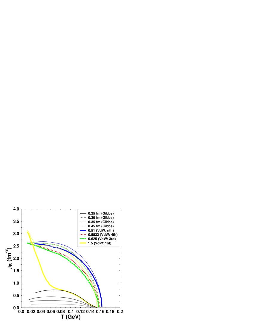
Figure 1: The phase transition diagram in the baryonic density and temperature ($\rho_{B}-T$) plane. The baryonic density is calculated for the hadronic phase below the phase transition line while for QGP is calculated above the phase transition line. The low thin lines show the phase diagram calculated using the Gibbs construction with various hadronic excluded volume. In Gibbs construction, Hagedorn bubbles (i.e. hadronic bubbles) are not included in the hadronic phase. The thick lines show $\rho^{HG}_{B}$ for the hadronic gas including Hagedorn bubbles with initial radii $r_{\mbox{FB}}=1.0$ fm. The Hagedorn bubbles’ internal color-flavor structure is given by Eq.(180). The bag constant is taken to be $B^{1/4}=210$ MeV. The above thin lines show $\rho^{QGP}_{B}$ for the QGP phase above the phase transition line for hadronic matter consisting Hagedorn bubbles with various internal color structure.

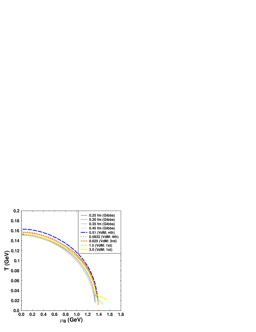
Figure 2: Same as Fig. 2 but in the baryonic chemical potential and temperature ($\mu_{B}-T$) plane. At low temperatures, the hadronic matter consisting both the hadronic mass spectrum particles and Hagedorn bubbles shift the phase transition line to larger chemical potentials than hadronic matter consisting only the hadronic mass spectrum particles. The bag constant for Hagedorn bubbles is taken to be $B^{1/4}=210$ MeV. The critical temperature $T_{c}(\mu_{B}=0)$ is found sensitive to $B$.

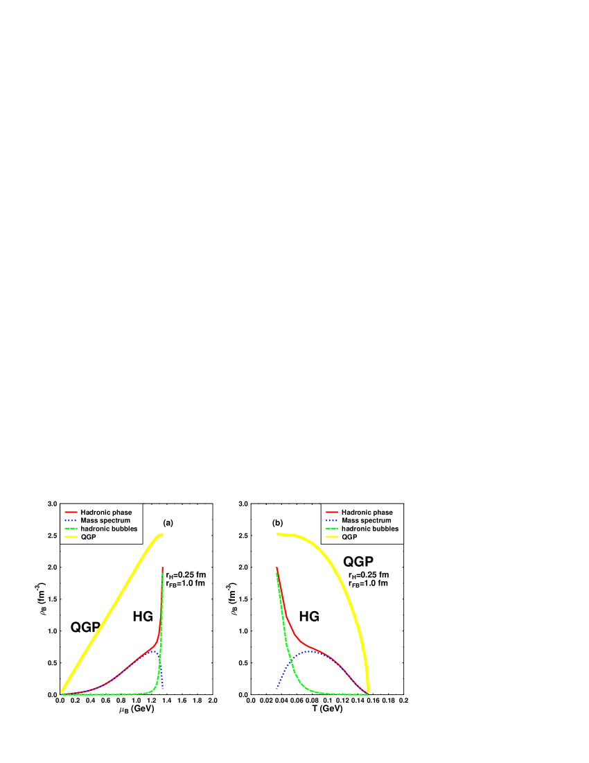
Figure 3: The baryonic densities for both Hagedorn bubbles (i.e. hadronic bubbles) and the hadronic mass spectra particles in the hadronic phase below the phase transition line. The above thick line shows the baryonic density $\rho^{QGP}_{B}$ for the QGP phase above the phase transition line for hadronic matter consisting hadronic mass spectrum particles and Hagedorn states with initial radius $r_{\mbox{FB}}=1.0$ fm for Hagedorn bubble’s volume fluctuation. The excluded volume for the hadronic mass spectrum particles is taken to be $r_{H}=0.25$ fm. At high temperatures and low chemical potentials, the hadronic mass spectrum particles is dominated while Hagedorn bubbles become the dominant for large chemical potentials and low temperatures. a) versus baryonic chemical potential $\mu_{B}$. b) versus temperature.

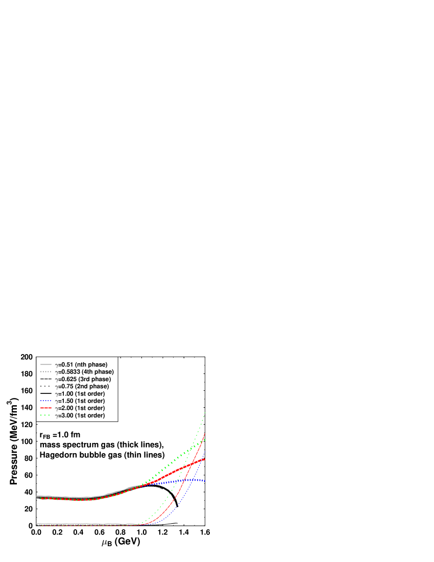
Figure 5: The pressure for the gas of hadronic mass spectrum particles and the pressure for the gas of Hagedorn states (i.e. hadronic bubbles) versus the baryonic chemical potential $\mu_{B}$ at temperatures just below the phase transition line. These pressures are displayed for Hagedorn bubbles with various values of internal color-flavor structure $\alpha=4\gamma-1$ factor of 0.5, 1.00, 1.50, 2.00 and 3.00 where the density of states is given by Eq.(180). It is shown that the gas pressure for Hagedorn bubbles becomes larger than that for the hadronic mass spectrum particles for large baryonic chemical potentials. The small excluded volume component for the mass spectrum particles and the large excluded volume component for Hagedorn states approximation is considered in the numerical calculations.

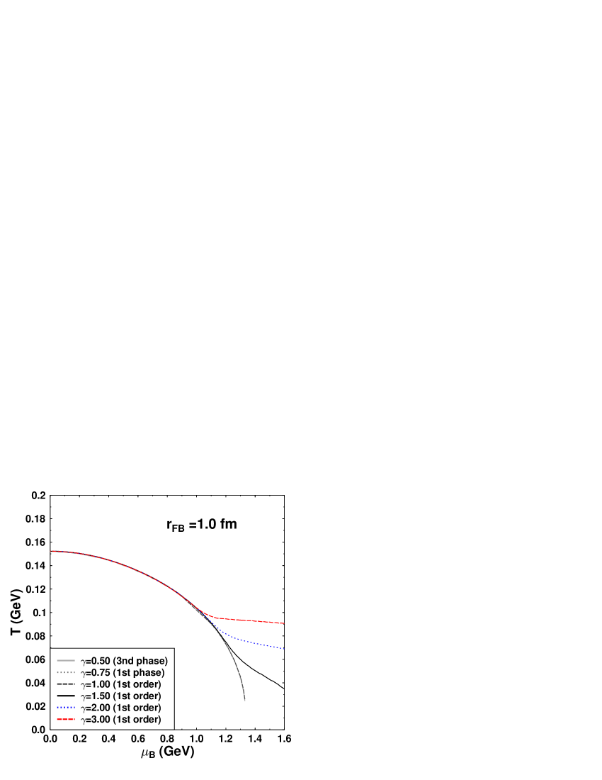
Figure 7: Same as Fig. 4 but for density of states including the volume fluctuation consistently as given in model (II) (see Eq.(194)).

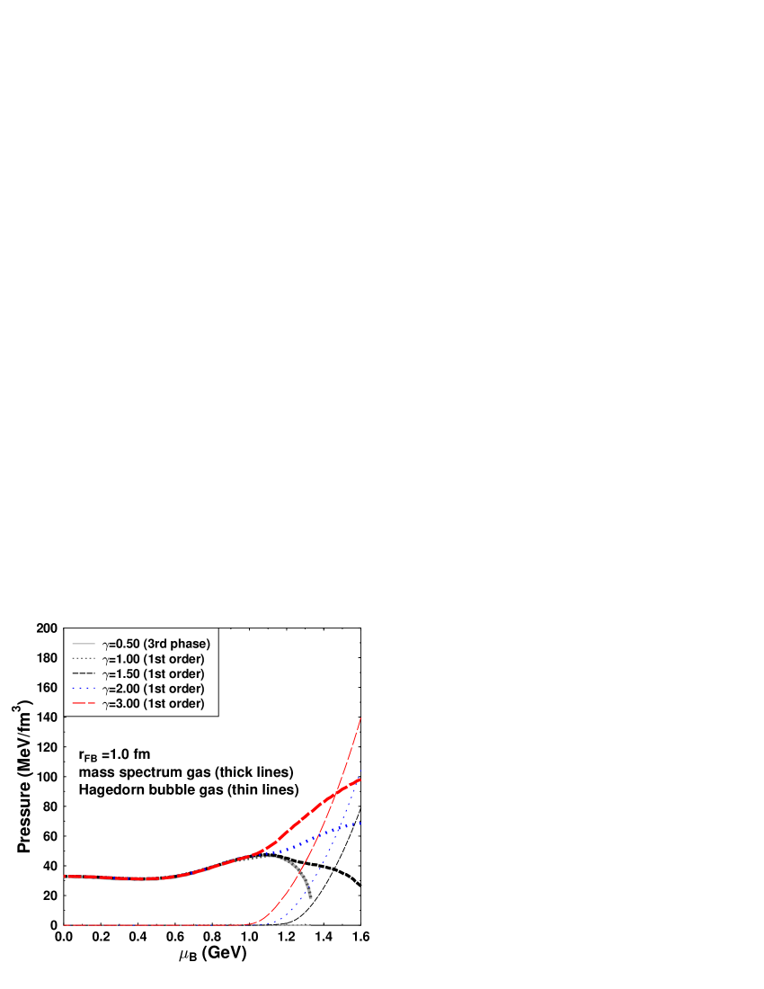
Figure 8: The same as Fig. 5 but for the density Eq.(194), i.e. model (II).

In the following, the hadronic matter is treated as Van der Waals gas consisting of all the known particles as given in the particle data group book et. al. (2004). Hereinafter, we call these particles the mass spectrum particles. The highly excited hadronic states are also taken into account and they are taken as Van der Waals gas of Hagedorn bubbles. The density of states for Hagedorn bubbles is derived from Laplace inverse of the mixed canonical ensemble of blob of quarks and gluons with specific internal color-flavor structure. These states are similar to Hagedorn states in the bootstrap model Hagedorn (1965); Frautschi (1971) where the density of states for the hadronic matter is modified significantly for the highly compressed or heated matter because the appearance of exotic hadronic (i.e. Hagedorn) bubbles with large masses $m_{H}>2.0$ GeV in the hadronic phase. The rich mass spectrum of Hagedorn states is essential for softening the equation of state in particular for a large baryonic chemical potential. In order to demonstrate the importance of Hagedorn bubbles in the hadronic phase, we have studied the quark-gluon plasma phase transition with and without Hagedorn bubbles. The effect of the initial volume fluctuation of Hagedorn bubbles in the phase transition is also considered. The density of states for Hagedorn bubbles is considered for the quark and gluon bags with various internal color-flavor symmetries range from colored bubbles (or colorless bubbles with the minimum color-flavor correlation) to singlet ones with strong color-flavor correlations specified by the parameter $\gamma_{\mbox{color}}\leq\gamma\leq\gamma_{\mbox{singlet}}\ll\gamma_{\mbox{strong}}$ and in the context of two approaches for the bubble’s volume fluctuation. The first approach is based on Gorenstein et. al. Gorenstein et al. (1984, 1982, 1983) ansatz for the maximum volume fluctuation while second one is based on Auberson et. al. Auberson et al. (1986a) ansatz for Gaussian like volume fluctuation. The bag constant for the hadronic pressure is taken $B^{1/4}=210\mbox{MeV}$ and the initial bag volume starts at $\frac{4}{3}\pi\left(1.0\mbox{fm}\right)^{3}$. In Figs. 1, 2 and 3, the one exclude volume component approximation is considered in the numerical calculations while the excluded volume with small and large volume components approximation is considered in Figs. 4, 5, 7 and 8.

We display the baryonic density and temperature $(\rho_{B}-T)$ phase transition diagram in Fig. 1. The thin lines depict the phase transition diagram for hadronic matter consisting of Van der Waals gas of the known particles without Hagedorn bubbles with various excluded volumes. In this approximation, the phase transition to quark-gluon plasma is calculated using the standard Gibbs construction scheme where the pressures and the chemical potentials are equal in both phases. The quark-gluon plasma is treated as an ideal gas of quarks and gluons. The excluded volume for the mass spectrum particles is taken ${v_{\mbox{VdW}}}_{H}=4v_{H}$ where $V_{H}=\frac{4}{3}\pi r^{3}_{H}$ and the phase transition diagrams are displayed for excluded volume radii $r_{\mbox{H}}$=0.25, 0.35, 0.40 and 0.45 fm. The number of particles per volume is reduced as the size of the excluded volume increases. The proper Van der Waals excluded volume is chosen to fit the phenomenology and it is taken to be rather small ${r_{\mbox{VdW}}}_{H}=4^{1/3}r_{H}$ $\approx$ 0.40-0.65 fm ($r_{H}\approx$ 0.25-0.45 fm). The classical Van der Waals excluded volume corresponds the phenomenological nucleon radius $r_{N}\approx$ 0.40-0.65 fm. On the other hand, the thick lines display the baryonic density for the hadronic matter consisting all the known hadronic spectrum particles in the particle data group book et. al. (2004) as well as the highly excited Hagedorn bubbles. The excluded volume for the known hadronic particles is taken to be $r_{H}=0.25\mbox{fm}$, i.e. ${r_{\mbox{VdW}}}=0.40\mbox{fm}$. The density of states for Hagedorn bubbles is taken as given in Eqs(98), (180) and (181). The initial volume fluctuation, $V_{0}$, for Hagedorn bubbles is taken $r_{\mbox{FB}}$=1.0 and the bubble’s Van der Waals excluded volume $V_{\mbox{VdW}Q}=4V_{0}$. These Hagedorn bubbles are also supposed to be the fireballs (FB) could appear in the hadronic phase. The bag constant for the Hagedorn bubble is taken $B^{1/4}=210\mbox{MeV}$. The internal symmetry for the color-flavor correlation in Hagedorn bag is chosen to be one for the massless flavorless and color singlet state, $\gamma$=1.5 with a smoothed volume fluctuation as given in Eq.(181). When Hagedorn bubbles are included in the calculation, the phase transition diagram is found self-consistently by searching the second singularity in the isobaric pressure. The first singularity is the extreme right singularity point in the limit of infinite external volume given by Eqs.(140) and (141), while the second singularity is for the isobaric pressure of Hagedorn bubbles. This second singularity is analogous to the condition for the phase transition determined by Hagedorn bubble’s mechanical instability arises when the bubble’s internal pressure reaches the external one from below. Due to this pressure instability, the bubbles start to expand rapidly and fill the entire space, consequently, quarks and gluons move freely and the phase transition to the quark-gluon plasma phase is reached. Fig. 1 shows that although the Van der Waals gas of the known hadronic mass spectrum particles without Hagedorn bubbles gives a reasonable phase transition diagram for low and intermediate densities, it fails to predict the phase transition for large baryonic density and low temperature. The finite size effect for the hadronic phase and quark-gluon plasma is also found important here Rafelski and Danos (1980); Rafelski and Letessier (2002); Pratt and Ruppert (2003). Including Van der Waals gas for color singlet bubbles $\gamma=\frac{3}{2}$ and bubbles with more complicated internal color-flavor structure $\gamma=3.0$ shifts the phase transition line to higher baryonic densities. The phase transition diagram exhibits a long “tail” at low temperatures and high densities. Furthermore, it is found that increasing the bubble’s initial volume suppresses Hagedorn bubbles population. This supports the intuitive idea that Hagedorn bubble spectrum is the continuation for the excited mass spectrum for the known hadronic particles found in the particle data group book et. al. (2004) where Hagedorn bubble mass spectrum starts at the end of the hadronic mass spectrum particles.

The above thin lines show the baryonic densities for the quark-gluon plasma phase $\rho^{QGP}_{B}$ above the phase transition point for hadronic matter consisting both the spectrum of known hadrons and Hagedorn bubbles with various internal color-flavor structures. It is shown that $\rho^{QGP}_{B}$ above the phase transition point exceeds significantly that for the hadronic gas $\rho^{HG}_{B}$ consisting the known hadronic particles and Hagedorn bubbles with internal structure $\gamma=1.5$ below the phase transition point. This measurable discrepancy in the baryonic density between two phases indicates a first order phase transition and a discontinuity in the baryonic density at the point of phase transition. However, the case is rather different for hadronic matter consisting Hagedorn bubbles with internal color-flavor structure $\gamma=0.51$ 0.5833 and 0.625. It is found that the split in baryonic density between two phases is tiny for $\gamma=0.51$ and small for 0.625. This could indicate a continuity for the baryonic density at the point of the phase transition and a discontinuity for higher derivatives of the thermodynamical grand potential density. Indeed the baryonic density split above and below the phase transition line sheds some information about the order of the phase transition and the discontinuity of the isobaric pressure and its first n-th derivatives. Indeed, it is supposed that the higher order phase transition reduces the split size at the point of the phase transition significantly where the isobaric pressure is continuous while its $n^{th}$ derivative is supposed to be discontinuous. Furthermore, the numerical calculations show that this density split decreases significantly as the internal structure decreases from $\gamma=1.5$ to $0.51$. This evidently indicates that the hadronic system consisting Hagedorn bubbles with internal structure $\gamma=1.5$ undergoes a first order phase transition while the system consisting bubbles with internal structure $\gamma=0.51$ undergoes a higher order phase transition and the $n^{th}$ higher derivatives of the thermodynamical grand potential density is continuous.

The phase transition diagram in the baryonic chemical potential and temperature $(T-\mu_{B})$ plane is displayed in Fig. 2. The phase transition line for the hadronic gas of only the known hadronic mass spectrum particles without any Hagedorn state ends at the chemical potential $\mu_{B}\approx 1300$ MeV for low temperatures. However, the size effect for the excluded volume in $T-\mu_{B}$ plane is not apparent as for the ($\rho_{B}-T$) phase transition diagram shown in Fig. 1. When Hagedorn bubbles are included, the phase transition diagram is shifted to larger baryonic chemical potentials for low temperatures. The phase transition diagram is modified to have a long tail at large baryonic chemical potentials and low temperatures. When Hagedorn bubbles appear in highly dense matter and low temperatures, the system prefers to stay in the hadronic phase which is dominated by highly compressed Hagedorn bubbles. Furthermore, the system experiences a smooth phase transition from hadronic gas dominated by the hadronic mass spectrum particles to another one dominated by foam of dense Hagedorn bubbles. The baryonic densities for both the mass spectrum particles $\rho^{HG:spectrum}_{B}$ and Hagedorn bubbles $\rho^{HG:FB}_{B}$ in the hadronic phase below the phase transition line to QGP are displayed in Fig. 3. We have also displayed the baryonic density $\rho^{QGP}_{B}$ for QGP above the line of the phase transition. It is shown that the hadronic gas of the hadronic mass spectrum particles dominates the hadronic phase for low and intermediate baryonic chemical potentials with temperatures higher than 60 MeV while Hagedorn bubbles become the dominant one in the hadronic phase for the chemical potential $\mu_{B}$ exceeds 1200 MeV and the temperature falls below 60 MeV.

As outlined in the previous sections, the density of states for Hagedorn bubbles is given by the microcanonical ensemble for blobs of quarks and gluons with specific color-flavor symmetry. The micro-canonical ensemble is derived from the inverse Laplace transform of the mixed grand canonical ensemble of quarks and gluons confined in a cavity. The micro-canonical ensemble measures the mass spectral density Eqs.(88) and (98) for Hagedorn bubble with specific volume for a cavity with sharp surface. The volume fluctuation can be calculated by finding a solution for a bag model with a deformed boundary and this solution is, in general, not known. The bag model with a smoothed boundary can be mimicked by using several assumptions to fit the phenomenology. For the nuclear shell model, the density of states is modified by using the ansatz of Strutinsky Strutinsky (1967, 1968); Balian and Bloch (1970, 1971, 1974) in order to fit the nuclear data and is based on smearing the delta function $\delta(E-E_{0})$ respecting energy conservation.

Here, we are going to study different scenarios for incorporating volume fluctuation and the phase transition impact on extending our previous discussions to more realistic systems. We emphasize in the following that the bubble’s color-flavor internal symmetry and its volume fluctuation plays a vital role in determining the order of the phase transition at low baryonic chemical potential and high temperature and the shape of the phase transition line at large chemical potential as well. In order to emphasize the volume fluctuation’s role in the phase transition we studied two models with different ansatz for the volume fluctuation.

In the model of Gorenstein et. al. Gorenstein et al. (1984, 1982, 1983) hereafter denoted as model (I), the volume fluctuation is measured by differentiating the microcanonical ensemble with respect to the bag’s volume (see Eq.(179)). This approximation leads to a smoothed volume fluctuation as given in Eq.(181) which is independent on the bubble’s volume and depends only on the bubble energy density. It is asymptotically equivalent to replacing the volume delta function $\delta(v-v_{0})$ given in Eq.(145) in the standard MIT bag by the power law $x^{3/4}$ where $x$ is the energy density. This variation is volume independent and subsequently it behaves the maximum volume fluctuation. We display the phase transition diagram in Fig. 4 with various values for Hagedorn bubble’s color-flavor correlation parameter, $\gamma$= 0.51, 0.5833, 0.625, 0.75, 1.0, 1.5, 2.0 and 3.0. The excluded volume for the mass spectrum particles is fixed to $r_{\mbox{H}}=0.30\mbox{fm}$ and Hagedorn bubbles’ initial volume fluctuation starts from $r_{\mbox{FB}}=1.0\mbox{fm}$. The $\gamma=0.5$ case corresponds to colored bubbles while $\gamma=1.5$ corresponds to color singlet bubbles. For values of $\gamma>1.5$ Hagedorn bubbles have more complicated color-flavor structures but still remain in a color singlet state, while for $\gamma<1.5$ the bubbles have color-flavor structure with color nonsinglet components. The cases with $\gamma=$ 0.51, 0.5833, 0.625, 0.75 or 1.0 do not alter the shape of the phase transition line for large baryonic chemical potential. The phase transition line ends at a baryonic chemical potential of $\mu_{B}\approx$ 1350 MeV for zero temperature. The order of the phase transition changes from 1st order to $2^{nd}$, $3^{rd}$, $4^{th}$ and $n^{th}$ order for $\gamma=$ 0.75, 0.625, 0.5833 and 0.51, respectively. For $\gamma=$ 1.5, 2.0 and 3.0, the phase transition diagram changes significantly and the phase transition line is shifted to larger baryonic chemical potential for low temperature. The shift of the phase transition line increases drastically with $\gamma$. However, in the one component excluded volume approximation (see Fig.2) this shift in the phase transition diagram to larger baryonic chemical potential at low temperature is less pronounced for $\gamma=1.5$ than that for the small and large excluded volume components approximation displayed in Fig.4. The reason is that the bubbles in the one excluded volume component approximation are effectively more suppressed than that for the small and large excluded volume components approximation. The system prefers to remain in the hadronic phase dominated by Hagedorn bubbles for large baryonic chemical potential rather than undergoes a phase transition to real deconfined quark-gluon plasma. When the medium becomes sufficiently hot, these Hagedorn bubbles undergo a phase transition to the quark-gluon plasma.

We display in Fig. 5 the pressures for the gas of all known nonstrange particles and the gas of Hagedorn bubbles versus the baryonic chemical potential $\mu_{B}$ at temperatures just below the phase transition diagram. The sum of both pressures gives the total pressure for the hadronic phase. Most of the thermodynamical quantities such as particle multiplicities are derived from the isobaric pressure. The thermodynamical grand potential density is also given in terms of the isobaric pressure. In the dilute hadronic matter, the pressure for Hagedorn bubble gas is suppressed and Hagedorn states unlikely appear in the hadronic phase. The gas of the hadronic mass spectrum particles is the dominant in the hadronic system for baryonic chemical potential up to $\mu_{B}\approx$ 1200 MeV. In this regime the colored bubbles with $\gamma=0.5$ are strongly suppressed. If these bubbles appear because of the high thermal excitations, their gas pressure diverges and whenever they appear they explode and occupy the entire space and mix with the hadronic mass spectrum particles instantly. This mechanism leads to the so called crossover phase transition. The bubbles with color nonsinglet components and exponents $\gamma\leq\frac{3}{4}$ may appear slightly just below the phase transition line and the system undergoes a higher order phase transition to quark-gluon plasma. These bubbles are also suppressed in the hadronic phase, their appearance just below the phase transition diagram allows a higher order phase transition. On the other hand, the bubbles with the net color singlet state do not appear for small and intermediate baryonic chemical potentials $\mu_{B}\leq$ 1000 MeV. When the baryonic chemical potential exceeds $\mu_{B}\geq 1000$ MeV, these Hagedorn bubbles appear and dominate the hadronic phase. For the small and intermediate baryonic chemical potential, Hagedorn states appear just below the phase transition line. Fig. 5 shows also that with increasing $\gamma$, the pressure for Hagedorn bubbles increases and the system prefers to remain in the hadronic phase for dense and cold nuclear matter. However, at high temperatures, the system undergoes a phase transition to quark-gluon plasma.

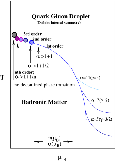
Figure 6: The sketch for the phase transition diagram outlining the shape and order of the phase transition between the hadronic and quark-gluon plasma phases. The hadronic gas consists all of the known hadronic mass spectrum particles and Hagedorn bubbles with various values for color-flavor correlations as determined by the pre-exponential power factor $\alpha=4\gamma-1$. The sketch is for model (I) with the density of states given by Eq.(180) (e.g. Hagedorn bubbles with strong volume fluctuation). The strength of the color-flavor correlation factor $\gamma\equiv\gamma(\mu)$ (e.g. $\alpha(\mu)$) changes the order of the phase transition for small baryonic chemical potentials and high temperatures while it modifies the shape of the phase transition at large chemical potentials and low temperatures. The phenomenological assumption is that the exponent $\gamma$ is modified self-consistently with respect to the baryonic chemical potential $\mu_{B}$. The variation of the phenomenological exponent $\gamma$ in the medium causes the existence of critical point in the phase transition diagram.

In order to summarize the scenario for the order and shape of the phase transition in model (I), the corresponding phase transition diagram is sketched in Fig. 6. Let us discuss the influence of the parameter $\alpha=4\gamma-1$ on changes to the phase transition diagram by varying it with the baryochemical potential. There is no phase transition for hadronic matter with $\alpha=1$ (e.g. bubbles structure $\gamma=0.5$) and the system undergoes a crossover phase transition to the quark-gluon plasma for dilute and hot matter. For slightly larger baryonic chemical potential, the system undergoes n-th order phase transition to quark-gluon plasma for $\alpha<2$ $\left(\gamma<\frac{3}{4}\right)$ as Hagedorn bubbles appear near the phase transition due to the thermal excitations. The first order phase transition takes place only for bubbles with $\alpha>2$. Hadronic matter consisting bubbles with $\alpha=2$ undergoes a second order phase transition while the hadronic matter consisting ones with $\alpha=3/2$ $(\gamma=0.625)$ undergoes a third order phase transition. Therefore, the hadronic matter consisting color singlet bubbles, which has internal structure $\gamma=3/2$ for gluons and massless flavorless quarks undergoes a first order phase transition. For example, the bubbles with specific baryonic and mesonic internal structures have $\gamma=3/2$ and $\gamma=13/8$ Auberson et al. (1986b), respectively, and bubbles with 6 massless flavors and 3 colors with exact $SU_{6,t}\rightarrow SU(3)\times SU(3)$ have $\gamma=6$ Auberson et al. (1986b). Therefore, it is expected that the strong color-flavor correlation will lead $\gamma\gg 1$ for three flavors with symmetry $SU(3)_{c}\times{SU(3)_{f}}_{L}\times{SU(3)_{f}}_{R}$ and for two flavors with symmetry $SU(3)_{c}\times{SU(2)_{f}}_{L}\times{SU(2)_{f}}_{R}$.

The basic question is we follow now at which extent do the color-flavor symmetry and the modification of the volume fluctuation affects the order and shape of the phase transition line. It is known from the nuclear shell theory Strutinsky (1967, 1968); Balian and Bloch (1970, 1971, 1974) that the deformation of the cavity boundary smears the density of states by smoothing the boundary surface. Auberson et. al. Auberson et al. (1986a) have argued that within the MIT bag model the mass fluctuates around the initial bag volume and it is approximated by Eq.(191). This procedure leads to the Gaussian-like volume fluctuation (see Eq.(195)). The resulting density of states for Hagedorn bubbles is given in Eq.(194). The quark and gluon bubble’s Gaussian volume fluctuation approach will be denoted as model (II). The phase transition diagram in the $(T-\mu_{B})$ plane is displayed in Fig. 7 for various internal color-flavor structures $\gamma=0.5$, 1.0, 1.5, 2.0 and 3.0. The excluded volume for the hadronic mass spectrum particles is taken to be $r_{\mbox{H}}=0.30\mbox{fm}$. The bubble’s initial volume fluctuation starts from $r_{\mbox{FB}}=1.0\mbox{fm}$.

Fig. 7 exhibits a first order phase transition for the colorless quark and gluon bubbles with $\gamma=\frac{3}{2}$ and also for bubbles with color nonsinglet components of $\frac{3}{2}>\gamma>\frac{5}{8}$, a second order phase transition for bubbles $\frac{5}{8}\geq\gamma>\frac{1}{2}$. A third order phase transition is found for colored bubbles with $\gamma=\frac{1}{2}$. This means that the third order phase transition is the maximum order. It takes place near the critical temperature $T\approx 155$ MeV where the hadronic mass spectrum gas undergoes a third order phase transition to real deconfined quark-gluon plasma. Hagedorn bubbles with a strong color-flavor correlation $\gamma\geq\frac{3}{2}$ but with net color singlet states trigger always a first order phase transition. Furthermore, the phase transition line for bubbles with color nonsinglet components and $\gamma<\frac{3}{2}$ are almost the same, although they undergo phase transitions of different order. The phase transition line drops at a chemical potential of $\mu_{B}\approx 1350$ MeV for low temperatures, $T\leq 100$ MeV. The interesting result to note in this scenario is, that the bubbles with specific internal color-flavor correlations and specific color components undergo a second order phase transition and that only colored bubbles undergo a third order phase transition. We would like to remind the reader that a specific flavor correlation has been introduced via the center of mass projection in order to reproduce the bootstrap density of states Kapusta (1982). The Lorenz structure of the center of mass projection is not invariant in the hot bath and can be broken partially or completely. This mechanism might modify the density of states. In the present model, we have assumed that this mechanism, in somehow, is absorbed by the phenomenological color-flavor parameter $\gamma$. The story is rather different for color singlet quark and gluon bags (i.e. Hagedorn bubbles) but with complicated color-flavor internal symmetries. Hagedorn bubbles with $\gamma=$ 1.5, 2.0 and 3.0 modify the phase transition diagram significantly and the system prefers to stay in the hadronic phase for large chemical potential and sufficiently low temperature. When the medium’s temperature exceeds $T=100~{}\mbox{MeV}$, the bubble color-flavor symmetry becomes less important to modify the shape of the phase transition line although it plays the vital role in determining the order of the phase transition. Hence, the phase transition diagram appear to be almost the same for Hagedorn bubbles with various color-flavor internal symmetries. This means that regardless of the bubbles internal color-flavor complications, quark-gluon droplets or plasma is formed.

We display in Fig. 8 the pressures for the gas of known spectrum particles and the gas of Hagedorn bubbles versus the baryonic chemical potential $\mu_{B}$ at temperatures just below the phase transition line. Hagedorn bubbles are strongly suppressed in diluted hadronic matter and they don’t appear at small baryonic chemical potential. They likely appear just below the phase transition line because of high thermal excitations of the medium. Furthermore, when the baryonic chemical potential increases and exceeds $\mu_{B}\approx 1000~{}\mbox{MeV}$, Hagedorn bubbles start to appear in the hadronic phase and their gas pressure increases significantly as the baryonic chemical potential increases. They becomes more dominant than the hadronic mass spectrum particle gas for highly compressed hadronic matter.

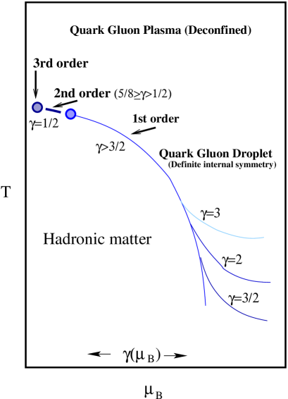
Figure 9: Sketch of the phase transition diagram as given in Fig. 6 but for density of states for model (II) as given by Eq.(194) (e.g. soft volume fluctuation). In this scenario the color-flavor correlation is determined by the power factor $\alpha=4\gamma-\frac{1}{2}$. The points $\gamma=3/2$ and $1/2$ correspond to a second and a third order phase transition, respectively. A first order phase transition takes place only for $\gamma>3/2$.

The sketch of the phase transition diagram for model (II) is depicted in Fig. 9. The parameter $\alpha=\left(4\gamma-\frac{1}{2}\right)$ is assumed to be modified in the medium and increases as the hadronic matter is compressed. In this scenario, the hadronic phase undergoes a third order phase transition to colored bubbles with $\alpha=1.5$ ($\gamma=0.5$) and forms real deconfined quark-gluon plasma in diluted and hot matter. The bubbles with color nonsinglet components with structure $2\geq\alpha>\frac{3}{2}$ (i.e. $\left(\frac{5}{8}\geq\gamma>\frac{1}{2}\right)$) have a second order phase transition while for $\frac{11}{2}>\alpha>2$ ($\left(\frac{3}{2}>\gamma>\frac{5}{8}\right)$) there appears a first order phase transition. The hadronic phase consisting Hagedorn states given by color singlet bubbles ($\gamma\geq 3/2$) undergoes a first order phase transition to quark-gluon droplets or plasma. Increasing the value of $\gamma$, modifies the phase transition diagram shape substantially in particular when the baryonic chemical potential becomes sufficiently large.

The comparison between phase transition scenarios for models (I) and (II) shows that the modification of Hagedorn bubble’s internal structure due to the interquark potential is important in order to draw and determine the order of the phase transition diagram. The interquarks potential modification could slightly deform the bag boundary and consequently the order of the phase transition even if the internal color-flavor symmetry remains intact.

Naively, Hagedorn bubble’s internal structure $\alpha$ (or $\gamma$) can also be modified in the medium. The rough sketch for the dependence of the phenomenological Hagedorn bubble’s internal structure $\gamma$ on the volume, temperature and chemical potential is depicted in Fig. 10. Primarily insight on melting the frozen internal color degrees of freedom in the medium have been given by Elze and Greiner Elze et al. (1984).

It is possible to go beyond the approximations of the previous models by considering higher order volume fluctuations or even finding a realistic hadronic bubble’s wavefunction. In this context, it is reasonable to assume that Hagedorn bubbles are thermally excited to higher quantum states whenever they appear. These highly excited Hagedorn bubbles can then even evaporate or emit smaller hadronic bubbles. In this case, the volume fluctuation becomes stronger and the bubble’s internal color-flavor structure is modified by smoothing the cavity boundary and consequently the density of states for Hagedorn states. When the phase transition takes place, the quark-gluon droplets continue to expand in the hot and diluted matter and then they eventually overlap with each other to form real deconfined quark-gluon plasma. On the other hand, in dense and cold hadronic matter the situation is rather different, however. When the baryonic chemical potential increases, the hadronic bubbles agglomerate and merge to form bubbles which are likely to have higher color-flavor symmetry and larger baryonic number. Hagedorn bubbles with simple symmetries merge and form dense bubbles with higher color-flavor symmetries and soften the equation of state. They shift the phase transition to higher density and temperature. At warm and large baryonic density, the system is dominated by Hagedorn bubbles. When these dense Hagedorn bubbles expand and overlap with each other, the system will undergo a phase transition to quark-gluon droplets. These droplets continue to expand and lose their internal color-flavor symmetry and then eventually they merge all together to form quark-gluon plasma.

The baryonic number for each Hagedorn bubble increases when the system is compressed and cooled and more dense Hagedorn bubbles with larger baryonic numbers appear in the system. At highly compressed matter, most of the baryonic density tends to concentrate in Hagedorn bubbles. However, the bubble’s size fluctuates smoothly and even shrinks in order to reduce the overlap effect with other hadronic bubbles. Hagedorn Bubbles with low mass density merge with other bubbles to form denser ones. When the maximum density is reached, the system undergoes a phase transition to Hagedorn bubbles foam. For low temperature and very dense matter, the bubble’s size can not shrink anymore due to the high constituent quarks and gluons pressure and the bubbles high surface tension in particular for cold matter. Hence the equation of state can be softened only by merging Hagedorn bubbles to form denser bubbles. Furthermore, the thermal excitation dissolves the surface between the bubbles spontaneously and subsequently the Hagedorn bubbles foam collapses to form quark-gluon plasma.

VIII Summary and conclusions

We have studied the order, shape and critical point for the phase transition diagram for hadronic matter consisting of all the known nonstrange hadronic particles and the highly excited hadronic bubbles correspond Hagedorn states those existed in the extreme conditions. The basic assumption is that Hagedorn bubble’s internal structure exponent $\gamma$ depends on the medium and may modify itself self-consistently with respect to $\mu_{B}$ in particular for temperature just below $T_{c}$. The exponent $\gamma$ is related to Hagedorn bubble’s internal color-flavor potential interaction. We have shown the order of the phase transition depends basically on the phenomenological exponent $\gamma$. We have demonstrated that both the volume fluctuation and the internal color-flavor structure for Hagedorn states play a crucial role in determining the order of the phase transition to quark-gluon droplets or plasma. It is found that Hagedorn bubbles’ quantum excitations modify the volume fluctuation by smoothing the quarks and gluons cavity boundary and subsequently change the order of the phase transition. The excited bubbles with smoothed surfaces cause a higher order phase transition. The order of the phase transition can be changed from a lower one to higher ones for the dilute and hot matter.

The phase transition is understood in the following way. Hagedorn bubbles are suppressed strongly in the dilute hadronic matter because the pressure of the hadronic mass spectrum particles is higher than the Hagedorn bubble’s internal pressure. These bubbles appear, however, due to the high thermal excitations. When their internal pressure exceeds the pressure of the gas of hadronic mass spectrum particles and other Hagedorn bubbles they start to expand at temperature just below the critical one. This expansion process depends on Hagedorn bubble’s volume fluctuation and its internal color-flavor symmetry as well. The bubbles with lower internal color-flavor symmetries are easily excited than those with more complicated internal color-flavor structures. On the other hand, Hagedorn bubbles become more dominant for the large baryonic chemical potential. When the hadronic gas is heated, the system passes a phase transition to quark-gluon plasma.

Naively, the bubble’s volume fluctuation depends on the reaction of the bubble’s constituent quarks and gluons to the medium. It is expected the bubble’s volume fluctuation becomes stronger in the dilute hadronic matter in particular near the critical temperature due to the high thermal excitations of the constituent particles. On the other hand, this volume fluctuation is supposed to be suppressed in the highly compressed matter in order to reduce the overlap effect among the hadrons. Two models for Hagedorn bubble’s volume fluctuation have been considered for bubbles with various internal color-flavor symmetries. The first model is the Gaussian volume distribution function while the second one is the maximal volume distribution function, e.g. smearing the delta function $\delta(v-v_{0})$ to volume independent function. It is shown that the strength of volume fluctuation is essential for a hadronic phase consisting bubbles with low internal color-flavor symmetries to undergo a higher order phase transition while the complexity of the bubble’s color-flavor symmetry is essential to determine the shape of the first order phase transition line for the large baryonic chemical potential. The variation of the exponent $\gamma(\mu_{B})$ in the medium for Hagedorn bubbles with specific internal color-flavor structures and the co-existence of the tri-critical point will be considered in the forthcoming work.

Figure 4: The phase transition diagram to QGP in the baryonic chemical potential and temperature ($\mu_{B}-T$) plane for the hadronic phase consisting all the known hadronic mass spectrum particles as well as Hagedorn bubbles (i.e. hadronic bubbles) with various color-flavor internal symmetry and a specific volume fluctuation as in the model (I) given in the text. The phase transition diagram is displayed for various values of the color-flavor structures as determined by the pre-exponential power $\gamma(\alpha)$ factor 0.5, 1.00, 1.50, 2.00 and 3.00. The hadronic phase is chosen to be an ideal gas of the hadronic mass spectrum particles with the excluded volume of $r_{H}$=0.30 fm as well as Hagedorn bubbles with an initial radii of $r_{\mbox{FB}}$=1.0 fm. The density of states for Hagedorn bubbles is given by Eq.(180). The small excluded volume component for the hadronic mass spectrum particles and the large excluded volume component for the Hagedorn states approximation is considered in the numerical calculations.

Figure 10: Rough Sketch of the dependence of Hagedorn bubble’s phenomenological internal structure parameter $\gamma\equiv\gamma(\mu_{B})$ on the volume, the temperature (or the energy in the microcanonical ensemble) and the chemical potential.