Hyperon-nucleon interactions – a chiral effective field theory approach

Abstract

We construct the leading order hyperon-nucleon potential in chiral effective field theory. We show that a good description of the available data is possible and discuss briefly further improvements of this scheme.

HISKP-TH-06/12, FZJ-IKP-TH-2006-14

, ,

1 Introduction

The derivation of nuclear interactions from chiral Effective Field Theory (EFT) has been discussed extensively in the literature since the work of Weinberg [1, 2]. For reviews we refer to [3, 4]. The main advantages of this scheme are the possibilities to derive two- and three- nucleon forces as well as external current operators in a consistent way and to improve calculations systematically by going to higher orders in the power counting.

Recently the nucleon-nucleon ($NN$) interaction has been described to a high precision using chiral EFT [5] (see also [6]). In this reference, the power counting is applied to the $NN$ potential, as originally proposed in [1, 2]. The $NN$ potential consists of pion-exchanges and a series of contact interactions with an increasing number of derivatives to parameterize the shorter ranged part of the $NN$ force. The pion-exchanges are treated nonperturbatively. A regularized Lippmann-Schwinger equation is solved to calculate observable quantities. Note that in contrast to the original Weinberg scheme, the effective potential is made explicitely energy-independent as it is important for applications in few-nucleon systems (for details, see [7]).

The hyperon-nucleon ($YN$) interaction has not been investigated using EFT as extensively as the $NN$ interaction. Hyperon and nucleon mass shifts in nuclear matter, using chiral perturbation theory, have been studied in [8]. These authors used a chiral interaction containing four-baryon contact terms and pseudoscalar-meson exchanges. Recently, the hypertriton and $\Lambda d$ scattering were investigated in the framework of an EFT with contact interactions [9]. Korpa et al. [10] performed a next-to-leading order (NLO) EFT analysis of $YN$ scattering and hyperon mass shifts in nuclear matter. Their tree-level amplitude contains four-baryon contact terms; pseudoscalar-meson exchanges were not considered explicitly, but ${\rm SU(3)}_{f}$ breaking by meson masses was modeled by incorporating dimension two terms coming from one-pion exchange. The full scattering amplitude was calculated using the Kaplan-Savage-Wise resummation scheme [11]. The hyperon-nucleon scattering data were described successfully for laboratory momenta below 200 MeV, using 12 free parameters. Some aspects of strong $\Lambda N$ scattering in effective field theory and its relation to various formulations of lattice QCD are discussed in [12].

In this work we apply the scheme used in [5] to the $YN$ interaction. Analogous to the $NN$ potential, at leading order in the power counting, the $YN$ potential consists of pseudoscalar-meson (Goldstone boson) exchanges and four-baryon contact terms, related via ${\rm SU(3)}_{f}$ symmetry. We solve a regularized coupled channels Lippmann-Schwinger equation for the leading-order (LO) $YN$ potential, including nonderivative contact terms and one-pseudoscalar-meson exchange, and fit to the low-energy cross sections, which are dominated by $S$-waves. Contrary to the $NN$ case, it is not possible to fit to partial waves, since they can not be extracted from the incomplete and low-precision $YN$ scattering data. We remark that our approach is quite different from [10].

The contents of this paper are as follows. The effective potential is developed in Section 2. In Section 2.1, we first give a brief recollection of the underlying power counting for the effective potential. We then investigate the ${\rm SU(3)}_{f}$ structure of the four-baryon contact interactions in leading order. This is done in Section 2.2. Here the lowest order ${\rm SU(3)}_{f}$-invariant four-baryon contact interactions are given and the corresponding potentials are derived. Similar to pion-exchanges in the $NN$ case, the $YN$ potential contains the exchanges of pseudoscalar mesons in general. The lowest order ${\rm SU(3)}_{f}$-invariant interactions are given in Section 2.3. Here also the one pseudoscalar meson-exchange potential is derived. The coupled channels Lippmann-Schwinger equation is solved for the partial-wave projected potential. This integral equation is solved in the LSJ basis. The Lippmann-Schwinger equation and the calculation of observable quantities are discussed in Section 3. Results of the fit to the low-energy $YN$ cross sections are presented in Section 4. Here we show the empirical and calculated total cross sections, differential cross sections and give the values for the scattering lengths. Also, predictions for some $YN$ phase shifts are shown and results for the hypertriton binding energy are presented. Finally, the summary presents an overview of the research in this work and an outlook for future investigations. Some technical details, of especially the partial wave projection, the LSJ-matrix elements and their derivations, are given in the appendices.

2 The effective potential

In this section, we construct in some detail the effective chiral hyperon-nucleon potential at leading order in the (modified) Weinberg power counting. This power counting is briefly recalled first. Then, we construct the minimal set of non-derivative four-baryon interactions and derive the formulae for the one-Goldstone-boson-exchange contributions.

2.1 Power counting

In this work, we apply the power counting to the effective hyperon-nucleon potential $V_{\rm eff}$ which is then injected into a regularized Lippmann-Schwinger equation to generate the bound and scattering states. The various terms in the effective potential are ordered according to

$$V_{\rm eff}\equiv V_{\rm eff}(Q,g,\mu)=\sum_{\nu}Q^{\nu}\,{\mathcal{V}}_{\nu}(Q/\mu,g)~{},$$ (2.1)

where $Q$ is the soft scale (either a baryon three-momentum, a Goldstone boson four-momentum or a Goldstone boson mass), $g$ is a generic symbol for the pertinent low–energy constants, $\mu$ a regularization scale, ${\mathcal{V}}_{\nu}$ is a function of order one, and $\nu\geq 0$ is the chiral power. It can be expressed as

$$\nu = 2-B+2L+\sum_{i}v_{i}\,\Delta_{i}~{},$$

$$\Delta_{i} = d_{i}+{\displaystyle\frac{1}{2}}\,b_{i}-2~{},$$ (2.2)

with $B$ the number of incoming (outgoing) baryon fields, $L$ counts the number of Goldstone boson loops, and $v_{i}$ is the number of vertices with dimension $\Delta_{i}$. The vertex dimension is expressed in terms of derivatives (or Goldstone boson masses) $d_{i}$ and the number of internal baryon fields $b_{i}$ at the vertex under consideration. The leading order (LO) potential is given by $\nu=0$, with $B=2$, $L=0$ and $\Delta_{i}=0$. Using Eq. (2.1) it is easy to see that this condition is fulfilled for two types of interactions – a) non-derivative four-baryon contact terms with $b_{i}=4$ and $d_{i}=0$ and b) one-meson exchange diagrams with the leading meson-baryon derivative vertices allowed by chiral symmetry ($b_{i}=2,d_{i}=1$). At LO, the effective potential is entirely given by these two types of contributions, which will be discussed in detail in the following chapters.

2.2 The four-baryon contact terms

The leading order contact term for the nucleon-nucleon ($NN$) interactions is given by [1, 7]

$${\mathcal{L}} = C_{i}\left(\bar{N}\Gamma_{i}N\right)\left(\bar{N}\Gamma_{i}N\right)\ ,$$ (2.3)

where $\Gamma_{i}$ are the usual elements of the Clifford algebra [13]

$$\Gamma_{1}=1\,,\,\,\Gamma_{2}=\gamma^{\mu}\,,\,\,\Gamma_{3}=\sigma^{\mu\nu}\,,\,\,\Gamma_{4}=\gamma^{\mu}\gamma_{5}\,,\,\,\Gamma_{5}=\gamma_{5}\,\,.$$ (2.4)

Considering the large components of the nucleon spinors only, the leading order contact term, Eq. (2.3), becomes

$${\mathcal{L}} = -\left(C_{1}+C_{2}\right)\left(\varphi^{\dagger}_{N}\varphi_{N}\right)\left(\varphi^{\dagger}_{N}\varphi_{N}\right)+\left(2C_{3}+C_{4}\right)\left(\varphi^{\dagger}_{N}\mbox{\boldmath$\sigma$}\varphi_{N}\right)\left(\varphi^{\dagger}_{N}\mbox{\boldmath$\sigma$}\varphi_{N}\right)$$ (2.5)

$$\equiv -\frac{1}{2}C_{S}\left(\varphi^{\dagger}_{N}\varphi_{N}\right)\left(\varphi^{\dagger}_{N}\varphi_{N}\right)-\frac{1}{2}C_{T}\left(\varphi^{\dagger}_{N}\mbox{\boldmath$\sigma$}\varphi_{N}\right)\left(\varphi^{\dagger}_{N}\mbox{\boldmath$\sigma$}\varphi_{N}\right)\ ,$$

where $\varphi_{N}$ are the large components of the nucleon Dirac spinor and $C_{S}$ and $C_{T}$ are constants that need to be determined by fitting to the experimental data.

In the case of the hyperon-nucleon ($YN$) interactions we will consider a similar but ${\rm SU(3)}_{f}$ invariant coupling. Thus, let us discuss the flavor structure of the contact terms for the $J^{P}=\frac{1}{2}^{+}$ octet baryons in the following. The leading order contact terms for the octet baryon-baryon interactions, that are Hermitian and invariant under Lorentz transformations, are given by the ${\rm SU(3)}_{f}$ invariants

$${\mathcal{L}}^{1} = {\tilde{C}}^{1}_{i}\left<\bar{B}_{a}\bar{B}_{b}\left(\Gamma_{i}B\right)_{a}\left(\Gamma_{i}B\right)_{b}\right>\ ,\quad{\mathcal{L}}^{2}={\tilde{C}}^{2}_{i}\left<\bar{B}_{a}\bar{B}_{b}\left(\Gamma_{i}B\right)_{b}\left(\Gamma_{i}B\right)_{a}\right>\ ,$$

$${\mathcal{L}}^{3} = {\tilde{C}}^{3}_{i}\left<\bar{B}_{a}\left(\Gamma_{i}B\right)_{a}\left(\Gamma_{i}B\right)_{b}\bar{B}_{b}\right>\ ,\quad{\mathcal{L}}^{4}={\tilde{C}}^{4}_{i}\left<\bar{B}_{a}\left(\Gamma_{i}B\right)_{a}\bar{B}_{b}\left(\Gamma_{i}B\right)_{b}\right>\ ,$$

$${\mathcal{L}}^{5} = {\tilde{C}}^{5}_{i}\left<\bar{B}_{a}\left(\Gamma_{i}B\right)_{b}\bar{B}_{b}\left(\Gamma_{i}B\right)_{a}\right>\ ,\quad{\mathcal{L}}^{6}={\tilde{C}}^{6}_{i}\left<\bar{B}_{a}\left(\Gamma_{i}B\right)_{b}\left(\Gamma_{i}B\right)_{a}\bar{B}_{b}\right>\ ,$$

$${\mathcal{L}}^{7} = {\tilde{C}}^{7}_{i}\left<\bar{B}_{a}\left(\Gamma_{i}B\right)_{a}\right>\left<\bar{B}_{b}\left(\Gamma_{i}B\right)_{b}\right>\ ,\quad{\mathcal{L}}^{8}={\tilde{C}}^{8}_{i}\left<\bar{B}_{a}\left(\Gamma_{i}B\right)_{b}\right>\left<\bar{B}_{b}\left(\Gamma_{i}B\right)_{a}\right>\ ,$$

$${\mathcal{L}}^{9} = {\tilde{C}}^{9}_{i}\left<\bar{B}_{a}\bar{B}_{b}\right>\vphantom{\bar{B}_{a}}\left<\left(\Gamma_{i}B\right)_{a}\left(\Gamma_{i}B\right)_{b}\vphantom{\bar{B}_{a}}\right>\ .$$ (2.6)

Here $a$ and $b$ denote the Dirac indices of the particles, $B$ is the usual irreducible octet representation of ${\rm SU(3)}_{f}$ given by

$$B = \left(\begin{array}[]{ccc}\frac{\Sigma^{0}}{\sqrt{2}}+\frac{\Lambda}{\sqrt{6}}&\Sigma^{+}&p\\ \Sigma^{-}&\frac{-\Sigma^{0}}{\sqrt{2}}+\frac{\Lambda}{\sqrt{6}}&n\\ -\Xi^{-}&\Xi^{0}&-\frac{2\Lambda}{\sqrt{6}}\end{array}\right)\ ,$$ (2.10)

and the brackets $\left<...\right>$ denote taking the trace in the three-dimensional flavor space. The Clifford algebra elements are here actually diagonal $3\times 3$-matrices in flavor space. Term 9 in Eq. (2.6) can be eliminated using the identity

$$-\left<\bar{B}_{a}\bar{B}_{b}\left(\Gamma_{i}B\right)_{a}\left(\Gamma_{i}B\right)_{b}\right>+\left<\bar{B}_{a}\bar{B}_{b}\left(\Gamma_{i}B\right)_{b}\left(\Gamma_{i}B\right)_{a}\right>$$

$$-\frac{1}{2}\left<\bar{B}_{a}\left(\Gamma_{i}B\right)_{b}\bar{B}_{b}\left(\Gamma_{i}B\right)_{a}\right>+\frac{1}{2}\left<\bar{B}_{a}\left(\Gamma_{i}B\right)_{a}\bar{B}_{b}\left(\Gamma_{i}B\right)_{b}\right>$$

$$=\frac{1}{2}\left<\bar{B}_{a}\left(\Gamma_{i}B\right)_{a}\right>\left<\bar{B}_{b}\left(\Gamma_{i}B\right)_{b}\right>-\frac{1}{2}\left<\bar{B}_{a}\left(\Gamma_{i}B\right)_{b}\right>\left<\bar{B}_{b}\left(\Gamma_{i}B\right)_{a}\right>$$

$$-\frac{1}{2}\left<\bar{B}_{a}\bar{B}_{b}\right>\vphantom{\bar{B}_{a}}\left<\left(\Gamma_{i}B\right)_{a}\left(\Gamma_{i}B\right)_{b}\vphantom{\bar{B}_{a}}\right>\ .$$ (2.11)

Making use of the trace property $\left<AB\right>=\left<BA\right>$, we see that the terms 3 and 6 in Eq. (2.6) are equivalent to the terms 2 and 1 respectively. Also making use of the Fierz theorem, Appendix A, one can show that the terms 1, 4 and 8 are equivalent to the terms 2, 5 and 7, respectively. So, we only need to consider the terms 2, 5 and 7. Writing these terms explicitly in the isospin basis we find for the $NN$ and $YN$ interactions

$${\mathcal{L}}^{2} = {\tilde{C}}^{2}_{i}\left\{\frac{1}{6}\left[5\left(\bar{\Lambda}\Gamma_{i}\Lambda\right)\left(\bar{N}\Gamma_{i}N\right)-4\left(\bar{\Lambda}\Gamma_{i}N\right)\left(\bar{N}\Gamma_{i}\Lambda\right)\right]\right.$$

$$+\frac{1}{2}\left[\left(\bar{\mbox{\boldmath$\Sigma$}}\cdot\Gamma_{i}\mbox{\boldmath$\Sigma$}\right)\left(\bar{N}\Gamma_{i}N\right)+i\left(\bar{\mbox{\boldmath$\Sigma$}}\times\Gamma_{i}\mbox{\boldmath$\Sigma$}\right)\cdot\left(\bar{N}\mbox{\boldmath$\tau$}\Gamma_{i}N\right)\right]$$

$$+\frac{1}{\sqrt{12}}\left[\left\{\left(\bar{N}\mbox{\boldmath$\tau$}\Gamma_{i}N\right)\cdot\left(\bar{\Lambda}\Gamma_{i}\mbox{\boldmath$\Sigma$}\right)+H.c.\right\}\right.$$

$$\left.\left.-2\left\{\left(\bar{N}\Gamma_{i}\mbox{\boldmath$\Sigma$}\right)\cdot\left(\bar{\Lambda}\mbox{\boldmath$\tau$}\Gamma_{i}N\right)+H.c.\right\}\right]\vphantom{\frac{1}{6}}\right\}\ ,$$

$${\mathcal{L}}^{5} = {\tilde{C}}^{5}_{i}\left\{\vphantom{\frac{1}{\sqrt{3}}}-\frac{1}{3}\left[\left(\bar{\Lambda}\Gamma_{i}\Lambda\right)\left(\bar{N}\Gamma_{i}N\right)+4\left(\bar{\Lambda}\Gamma_{i}N\right)\left(\bar{N}\Gamma_{i}\Lambda\right)\right]\right.$$

$$-\left[\left(\bar{\mbox{\boldmath$\Sigma$}}\cdot\Gamma_{i}\mbox{\boldmath$\Sigma$}\right)\left(\bar{N}\Gamma_{i}N\right)-i\left(\bar{\mbox{\boldmath$\Sigma$}}\times\Gamma_{i}\mbox{\boldmath$\Sigma$}\right)\cdot\left(\bar{N}\mbox{\boldmath$\tau$}\Gamma_{i}N\right)\right]$$

$$\left.-\frac{1}{\sqrt{3}}\left[\left(\bar{N}\mbox{\boldmath$\tau$}\Gamma_{i}N\right)\cdot\left(\bar{\Lambda}\Gamma_{i}\mbox{\boldmath$\Sigma$}\right)+H.c.\right]-\left(\bar{N}\Gamma_{i}N\right)\left(\bar{N}\Gamma_{i}N\right)\right\}\ ,$$

$${\mathcal{L}}^{7} = {\tilde{C}}^{7}_{i}\left\{2\left(\bar{\Lambda}\Gamma_{i}\Lambda\right)\left(\bar{N}\Lambda N\right)+2\left(\bar{\mbox{\boldmath$\Sigma$}}\cdot\Gamma_{i}\mbox{\boldmath$\Sigma$}\right)\left(\bar{N}\Gamma_{i}N\right)+\left(\bar{N}\Gamma_{i}N\right)\left(\bar{N}\Gamma_{i}N\right)\right\}\ .$$

Here $H.c.$ denotes the Hermitian conjugate of the specific term. Also we have introduced the isospinors and isovector according to

$$N=\left(\begin{array}[]{r}p\\ n\end{array}\right)\ ,\ \ \Xi=\left(\begin{array}[]{r}\Xi^{0}\\ \Xi^{-}\end{array}\right)\ .$$ (2.13)

The phases have been chosen according to [14], such that the inner product of the isovector $\Sigma$ is

$$\mbox{\boldmath$\Sigma$}\cdot\mbox{\boldmath$\Sigma$}=\Sigma^{+}\Sigma^{-}+\Sigma^{0}\Sigma^{0}+\Sigma^{-}\Sigma^{+}\ .$$ (2.14)

In order to find the interaction Lagrangian in a more symmetric form (with respect to Fierz rearranged terms like $\left(\bar{\Lambda}\Gamma_{i}N\right)\left(\bar{N}\Gamma_{i}\Lambda\right)$) we add to ${\mathcal{L}}^{2}$ and ${\mathcal{L}}^{5}$ their Fierz rearranged versions and perform a Fierz rearrangement. We find for the $NN$ and $YN$ interactions the Lagrangians

$${\mathcal{L}}^{2} = \frac{C^{2}_{i}}{2}\left\{\vphantom{\frac{1}{\sqrt{3}}}\frac{1}{3}\left(\bar{\Lambda}\Gamma_{i}\Lambda\right)\left(\bar{N}\Gamma_{i}N\right)+\left[\left(\bar{\mbox{\boldmath$\Sigma$}}\cdot\Gamma_{i}\mbox{\boldmath$\Sigma$}\right)\left(\bar{N}\Gamma_{i}N\right)\right.\right.$$

$$\left.\left.+i\left(\bar{\mbox{\boldmath$\Sigma$}}\times\Gamma_{i}\mbox{\boldmath$\Sigma$}\right)\cdot\left(\bar{N}\mbox{\boldmath$\tau$}\Gamma_{i}N\right)\right]-\frac{1}{\sqrt{3}}\left[\left(\bar{N}\mbox{\boldmath$\tau$}\Gamma_{i}N\right)\cdot\left(\bar{\Lambda}\Gamma_{i}\mbox{\boldmath$\Sigma$}\right)+H.c.\right]\right\}\ ,$$

$${\mathcal{L}}^{5} = -C^{5}_{i}\left\{\frac{5}{3}\left(\bar{\Lambda}\Gamma_{i}\Lambda\right)\left(\bar{N}\Gamma_{i}N\right)+\left[\left(\bar{\mbox{\boldmath$\Sigma$}}\cdot\Gamma_{i}\mbox{\boldmath$\Sigma$}\right)\left(\bar{N}\Gamma_{i}N\right)\right.\right.$$

$$\left.-i\left(\bar{\mbox{\boldmath$\Sigma$}}\times\Gamma_{i}\mbox{\boldmath$\Sigma$}\right)\cdot\left(\bar{N}\mbox{\boldmath$\tau$}\Gamma_{i}N\right)\right]+\frac{1}{\sqrt{3}}\left[\left(\bar{N}\mbox{\boldmath$\tau$}\Gamma_{i}N\right)\cdot\left(\bar{\Lambda}\Gamma_{i}\mbox{\boldmath$\Sigma$}\right)+H.c.\right]$$

$$\left.+\left(\bar{N}\Gamma_{i}N\right)\left(\bar{N}\Gamma_{i}N\right)\vphantom{\frac{5}{3}}\right\}\ ,$$

$${\mathcal{L}}^{7} = C^{7}_{i}\left\{2\left(\bar{\Lambda}\Gamma_{i}\Lambda\right)\left(\bar{N}\Lambda N\right)+2\left(\bar{\mbox{\boldmath$\Sigma$}}\cdot\Gamma_{i}\mbox{\boldmath$\Sigma$}\right)\left(\bar{N}\Gamma_{i}N\right)+\left(\bar{N}\Gamma_{i}N\right)\left(\bar{N}\Gamma_{i}N\right)\right\}\ .$$

This is the case for the flavor symmetric interaction (i.e. the ${}^{1}S_{0}$ wave). For the flavor antisymmetric interaction (i.e. the ${}^{3}S_{1}$ wave) we should have subtracted their Fierz rearranged versions. The leading order $YN$ contact terms given by these interactions are shown diagrammatically in Figure 2.1.

Figure 2.1: Lowest order contact terms for hyperon-nucleon interactions

If we consider again only the large components of the Dirac spinors in Eq. (2.2) then we need, similar to Eq. (2.5), six contact constants ($C^{2}_{S}$, $C^{2}_{T}$, $C^{5}_{S}$, $C^{5}_{T}$, $C^{7}_{S}$ and $C^{7}_{T}$,) for the $BB$ interactions. The (leading order) contact term potential resulting from the interaction Lagrangian Eq. (2.2) now becomes

$$V^{(0)} = C^{BB}_{S}+C^{BB}_{T}\ \mbox{\boldmath$\sigma$}_{1}\cdot\mbox{\boldmath$\sigma$}_{2}\ ,$$ (2.16)

where the coupling constants $C^{BB}_{S}$ and $C^{BB}_{T}$ for the flavor symmetric interaction are defined as

$$C^{NN}_{S,T} = -C^{5}_{S,T}+C^{7}_{S,T}\ ,$$

$$C^{\Lambda\Lambda}_{S,T} = \frac{1}{6}C^{2}_{S,T}-\frac{5}{3}C^{5}_{S,T}+2C^{7}_{S,T}\ ,$$

$$C^{\Lambda\Sigma}_{S,T} = -\frac{1}{\sqrt{3}}\left(\frac{C^{2}_{S,T}}{2}+C^{5}_{S,T}\right)\ ,$$

$$C^{\Sigma\Sigma}_{S,T} = \frac{C^{2}_{S,T}}{2}-C^{5}_{S,T}+2C^{7}_{S,T}\ .$$ (2.17)

For the flavor antisymmetric interaction the coupling constants $C^{BB}_{S}$ and $C^{BB}_{T}$ are defined as

$$C^{NN}_{S,T} = C^{5}_{S,T}+C^{7}_{S,T}\ ,$$

$$C^{\Lambda\Lambda}_{S,T} = \frac{3}{2}C^{2}_{S,T}+C^{5}_{S,T}+2C^{7}_{S,T}\ ,$$

$$C^{\Lambda\Sigma}_{S,T} = -\frac{1}{\sqrt{3}}\left(-\frac{3}{2}C^{2}_{S,T}+C^{5}_{S,T}\right)\ ,$$

$$C^{\Sigma\Sigma}_{S,T} = \frac{C^{2}_{S,T}}{2}-C^{5}_{S,T}+2C^{7}_{S,T}\ .$$ (2.18)

However, the coupling constants $C^{i}_{S,T}$ in Eqs. (2.17) and (2.18) still need to be multiplied with the isospin factors given in Table 2.1.

Table 2.1: The isospin factors for the various contact terms.

Channel	Isospin	$C^{2}_{S,T}$	$C^{5}_{S,T}$	$C^{7}_{S,T}$
$NN\rightarrow NN$	0	-	2	2
	1	-	2	2
$\Lambda N\rightarrow\Lambda N$	$\frac{1}{2}$	1	1	1
$\Lambda N\rightarrow\Sigma N$	$\frac{1}{2}$	-$\sqrt{3}$	-$\sqrt{3}$	-
$\Sigma N\rightarrow\Sigma N$	$\frac{1}{2}$	3	-1	1
	$\frac{3}{2}$	0	2	1

The $NN$ partial wave potentials now become

$$V^{NN}_{1S0} = 4\pi\left[-2\left(C^{5}_{S}-3C^{5}_{T}\right)+2\left(C^{7}_{S}-3C^{7}_{T}\right)\right]=V^{27},$$

$$V^{NN}_{3S1} = 4\pi\left[2\left(C^{5}_{S}+C^{5}_{T}\right)+2\left(C^{7}_{S}+C^{7}_{T}\right)\right]=V^{10^{*}}.$$ (2.19)

The $YN$ partial wave potentials become for $\Lambda N\rightarrow\Lambda N$

$$V^{\Lambda\Lambda}_{1S0} = 4\pi\left[\frac{1}{6}\left(C^{2}_{S}-3C^{2}_{T}\right)-\frac{5}{3}\left(C^{5}_{S}-3C^{5}_{T}\right)+2\left(C^{7}_{S}-3C^{7}_{T}\right)\right]$$

$$=\frac{1}{10}\left(9V^{27}+V^{8s}\right),$$

$$V^{\Lambda\Lambda}_{3S1} = 4\pi\left[\frac{3}{2}\left(C^{2}_{S}+C^{2}_{T}\right)+\left(C^{5}_{S}+C^{5}_{T}\right)+2\left(C^{7}_{S}+C^{7}_{T}\right)\right]$$ (2.20)

$$=\frac{1}{2}\left(V^{8a}+V^{10^{*}}\right),$$

for isospin-3/2 $\Sigma N\rightarrow\Sigma N$

$$V^{\Sigma\Sigma}_{1S0} = 4\pi\left[-2\left(C^{5}_{S}-3C^{5}_{T}\right)+2\left(C^{7}_{S}-3C^{7}_{T}\right)\right]=V^{27},$$

$$V^{\Sigma\Sigma}_{3S1} = 4\pi\left[-2\left(C^{5}_{S}+C^{5}_{T}\right)+2\left(C^{7}_{S}+C^{7}_{T}\right)\right]=V^{10},$$ (2.21)

for isospin-1/2 $\Sigma N\rightarrow\Sigma N$

$$\widetilde{V}^{\Sigma\Sigma}_{1S0} = 4\pi\left[\frac{3}{2}\left(C^{2}_{S}-3C^{2}_{T}\right)+\left(C^{5}_{S}-3C^{5}_{T}\right)+2\left(C^{7}_{S}-3C^{7}_{T}\right)\right]$$

$$=\frac{1}{10}\left(V^{27}+9V^{8s}\right),$$

$$\widetilde{V}^{\Sigma\Sigma}_{3S1} = 4\pi\left[\frac{3}{2}\left(C^{2}_{S}+C^{2}_{T}\right)+\left(C^{5}_{S}+C^{5}_{T}\right)+2\left(C^{7}_{S}+C^{7}_{T}\right)\right]$$ (2.22)

$$=\frac{1}{2}\left(V^{8a}+V^{10^{*}}\right),$$

and for $\Lambda N\rightarrow\Sigma N$

$$V^{\Lambda\Sigma}_{1S0} = 4\pi\left[\frac{1}{2}\left(C^{2}_{S}-3C^{2}_{T}\right)+\left(C^{5}_{S}-3C^{5}_{T}\right)\right]=\frac{3}{10}\left(-V^{27}+V^{8s}\right),$$

$$V^{\Lambda\Sigma}_{3S1} = 4\pi\left[-\frac{3}{2}\left(C^{2}_{S}+C^{2}_{T}\right)+\left(C^{5}_{S}+C^{5}_{T}\right)\right]=\frac{1}{2}\left(-V^{8a}+V^{10^{*}}\right).$$ (2.23)

The last part of the previous expressions gives explicitly the ${\rm SU(3)}_{f}$ representation of the potentials. We note that only 5 of the $\{8\}\times\{8\}=\{27\}+\{10\}+\{10^{*}\}+\{8\}_{s}+\{8\}_{a}+\{1\}$ representations are relevant for $NN$ and $YN$ interactions; equivalently, the six contact terms, $C_{S}^{2}$, $C_{T}^{2}$, $C_{S}^{5}$, $C_{T}^{5}$, $C_{S}^{7}$, $C_{T}^{7}$, enter the $NN$ and $YN$ potentials in only 5 different combinations. These 5 contact terms need to be determined by a fit to the experimental data. Since the $NN$ data can not be described with a LO EFT, see [1, 15], we will not consider the $NN$ interaction explicitly. Therefore, we consider the $YN$ partial wave potentials

$$V^{\Lambda\Lambda}_{1S0} = C^{\Lambda\Lambda}_{1S0}\ ,\quad V^{\Lambda\Lambda}_{3S1}=C^{\Lambda\Lambda}_{3S1}\ ,$$

$$V^{\Sigma\Sigma}_{1S0} = C^{\Sigma\Sigma}_{1S0}\ ,\quad V^{\Sigma\Sigma}_{3S1}=C^{\Sigma\Sigma}_{3S1}\ ,$$

$$\widetilde{V}^{\Sigma\Sigma}_{1S0} = 9C^{\Lambda\Lambda}_{1S0}-8C^{\Sigma\Sigma}_{1S0}\ ,\quad\widetilde{V}^{\Sigma\Sigma}_{3S1}=C^{\Lambda\Lambda}_{3S1}\ ,$$

$$V^{\Lambda\Sigma}_{1S0} = 3\left(C^{\Lambda\Lambda}_{1S0}-C^{\Sigma\Sigma}_{1S0}\right)\ ,\quad V^{\Lambda\Sigma}_{3S1}=C^{\Lambda\Sigma}_{3S1}\ .$$ (2.24)

We have chosen to search for $C^{\Lambda\Lambda}_{1S0}$, $C^{\Lambda\Lambda}_{3S1}$, $C^{\Sigma\Sigma}_{1S0}$, $C^{\Sigma\Sigma}_{1S0}$, and $C^{\Lambda\Sigma}_{3S1}$ in the fitting procedure. The other three partial wave potentials are then determined by ${\rm SU(3)}_{f}$-symmetry.

2.3 One pseudoscalar-meson exchange

The lowest order ${\rm SU(3)}_{f}$-invariant pseudoscalar-meson-baryon interaction Lagrangian with the appropriate symmetries is given by (see, e.g., [16]),

$${\mathcal{L}} = \left<i\bar{B}\gamma^{\mu}D_{\mu}B-M_{0}\bar{B}B+\frac{D}{2}\bar{B}\gamma^{\mu}\gamma_{5}\left\{u_{\mu},B\right\}+\frac{F}{2}\bar{B}\gamma^{\mu}\gamma_{5}\left[u_{\mu},B\right]\right>\ ,$$ (2.25)

with $M_{0}$ the octet baryon mass in the chiral limit. There are two possibilities for coupling the axial vector $u_{\mu}$ to the baryon bilinear. The conventional coupling constants $F$ and $D$, used here, satisfy the relation $F+D=g_{A}\simeq 1.26$. The axial-vector strength $g_{A}$ is measured in neutron $\beta$–decay. The covariant derivative acting on the baryons is

$$D_{\mu}B = \partial_{\mu}B+\left[\Gamma_{\mu},B\right]\ ,$$

$$\Gamma_{\mu} = \frac{1}{2}\left[u^{\dagger}\partial_{\mu}u+u\partial_{\mu}u^{\dagger}\right]\ ,$$

$$u^{2} = U=\exp(2iP/\sqrt{2}F_{\pi})\ ,$$ (2.26)

where $F_{\pi}$ is the weak pion decay constant, $F_{\pi}=92.4$ MeV, and $P$ is the irreducible octet representation of ${\rm SU(3)}_{f}$ for the pseudoscalar mesons (the Goldstone bosons)

$$P = \left(\begin{array}[]{ccc}\frac{\pi^{0}}{\sqrt{2}}+\frac{\eta}{\sqrt{6}}&\pi^{+}&K^{+}\\ \pi^{-}&\frac{-\pi^{0}}{\sqrt{2}}+\frac{\eta}{\sqrt{6}}&K^{0}\\ -K^{-}&\bar{K}^{0}&-\frac{2\eta}{\sqrt{6}}\end{array}\right)\ .$$ (2.30)

Symmetry breaking in the decay constants, e.g. $F_{\pi}\neq F_{K}$, formally appears at NLO and will not be considered in the following. The axial-vector $u_{\mu}$ is defined as

$$\frac{1}{2}u_{\mu} = \frac{i}{2}\left(u^{\dagger}\partial_{\mu}u-u\partial_{\mu}u^{\dagger}\right)=\frac{i}{2}\left\{u^{\dagger},\partial_{\mu}u\right\}=\frac{i}{2}u^{\dagger}\partial_{\mu}Uu^{\dagger}\ .$$ (2.31)

We remark that the first term in the interaction Lagrangian Eq. (2.25) leads to the Weinberg-Tomozawa terms, while the two last terms will lead to one-pseudoscalar-meson exchanges, which are of interest for the leading order potential. To evaluate one-pseudoscalar-meson exchange, we write down Eq. (2.31) explicitly and find for the term with the minimal number of pseudoscalar mesons

$$\frac{1}{2}u_{\mu} = -\frac{\partial_{\mu}P}{\sqrt{2}F_{\pi}}\ .$$ (2.32)

Now we find for the last two terms in Eq. (2.25) the derivative coupling interaction Lagrangian, leading to one-pseudoscalar-meson-exchange diagrams,

$${\mathcal{L}} = \left<\frac{D}{2}\bar{B}\gamma^{\mu}\gamma_{5}\left\{u_{\mu},B\right\}+\frac{F}{2}\bar{B}\gamma^{\mu}\gamma_{5}\left[u_{\mu},B\right]\right>$$ (2.33)

$$= -\left<\frac{g_{A}(1-\alpha)}{\sqrt{2}F_{\pi}}\bar{B}\gamma^{\mu}\gamma_{5}\left\{\partial_{\mu}P,B\right\}+\frac{g_{A}\alpha}{\sqrt{2}F_{\pi}}\bar{B}\gamma^{\mu}\gamma_{5}\left[\partial_{\mu}P,B\right]\right>\ .$$

Here we have defined $\alpha=F/(F+D)$ and $g_{A}=F+D$. Writing this interaction Lagrangian explicitly in the isospin basis, we find

$${\mathcal{L}} = -f_{NN\pi}\bar{N}\gamma^{\mu}\gamma_{5}\mbox{\boldmath$\tau$}N\cdot\partial_{\mu}\mbox{\boldmath$\pi$}+if_{\Sigma\Sigma\pi}\bar{\mbox{\boldmath$\Sigma$}}\gamma^{\mu}\gamma_{5}\times{\mbox{\boldmath$\Sigma$}}\cdot\partial_{\mu}\mbox{\boldmath$\pi$}$$ (2.34)

$$-f_{\Lambda\Sigma\pi}\left[\bar{\Lambda}\gamma^{\mu}\gamma_{5}{\mbox{\boldmath$\Sigma$}}+\bar{\mbox{\boldmath$\Sigma$}}\gamma^{\mu}\gamma_{5}\Lambda\right]\cdot\partial_{\mu}\mbox{\boldmath$\pi$}-f_{\Xi\Xi\pi}\bar{\Xi}\gamma^{\mu}\gamma_{5}\mbox{\boldmath$\tau$}\Xi\cdot\partial_{\mu}\mbox{\boldmath$\pi$}$$

$$-f_{\Lambda NK}\left[\bar{N}\gamma^{\mu}\gamma_{5}\Lambda\partial_{\mu}K+\bar{\Lambda}\gamma^{\mu}\gamma_{5}N\partial_{\mu}K^{\dagger}\right]$$

$$-f_{\Xi\Lambda K}\left[\bar{\Xi}\gamma^{\mu}\gamma_{5}\Lambda\partial_{\mu}K_{c}+\bar{\Lambda}\gamma^{\mu}\gamma_{5}\Xi\partial_{\mu}K_{c}^{\dagger}\right]$$

$$-f_{\Sigma NK}\left[\bar{\mbox{\boldmath$\Sigma$}}\cdot\gamma^{\mu}\gamma_{5}\partial_{\mu}K^{\dagger}\mbox{\boldmath$\tau$}N+\bar{N}\gamma^{\mu}\gamma_{5}\mbox{\boldmath$\tau$}\partial_{\mu}K\cdot{\mbox{\boldmath$\Sigma$}}\right]$$

$$-f_{\Sigma\Xi K}\left[\bar{\mbox{\boldmath$\Sigma$}}\cdot\gamma^{\mu}\gamma_{5}\partial_{\mu}K_{c}^{\dagger}\mbox{\boldmath$\tau$}\Xi+\bar{\Xi}\gamma^{\mu}\gamma_{5}\mbox{\boldmath$\tau$}\partial_{\mu}K_{c}\cdot{\mbox{\boldmath$\Sigma$}}\right]-f_{NN\eta_{8}}\bar{N}\gamma^{\mu}\gamma_{5}N\partial_{\mu}\eta$$

$$-f_{\Lambda\Lambda\eta_{8}}\bar{\Lambda}\gamma^{\mu}\gamma_{5}\Lambda\partial_{\mu}\eta-f_{\Sigma\Sigma\eta_{8}}\bar{\mbox{\boldmath$\Sigma$}}\cdot\gamma^{\mu}\gamma_{5}{\mbox{\boldmath$\Sigma$}}\partial_{\mu}\eta-f_{\Xi\Xi\eta_{8}}\bar{\Xi}\gamma^{\mu}\gamma_{5}\Xi\partial_{\mu}\eta\ .$$

We have introduced the isospin doublets

$$N=\left(\begin{array}[]{r}p\\ n\end{array}\right)\ ,\ \ \Xi=\left(\begin{array}[]{r}\Xi^{0}\\ \Xi^{-}\end{array}\right)\ ,\ \ K=\left(\begin{array}[]{r}K^{+}\\ K^{0}\end{array}\right)\ ,\ \ K_{c}=\left(\begin{array}[]{r}\bar{K}^{0}\\ -K^{-}\end{array}\right)\ .$$ (2.35)

The interaction Lagrangian in Eq. (2.34) is invariant under $SU_{f}(3)$ transformations if the various coupling constants are expressed in terms of the coupling constant $f\equiv g_{A}/2F_{\pi}$ and the $F/(F+D)$-ratio $\alpha$ as [14],

$$\begin{array}[]{rlrlrl}f_{NN\pi}=&f,&f_{NN\eta_{8}}=&\frac{1}{\sqrt{3}}(4\alpha-1)f,&f_{\Lambda NK}=&-\frac{1}{\sqrt{3}}(1+2\alpha)f,\\ f_{\Xi\Xi\pi}=&-(1-2\alpha)f,&f_{\Xi\Xi\eta_{8}}=&-\frac{1}{\sqrt{3}}(1+2\alpha)f,&f_{\Xi\Lambda K}=&\frac{1}{\sqrt{3}}(4\alpha-1)f,\\ f_{\Lambda\Sigma\pi}=&\frac{2}{\sqrt{3}}(1-\alpha)f,&f_{\Sigma\Sigma\eta_{8}}=&\frac{2}{\sqrt{3}}(1-\alpha)f,&f_{\Sigma NK}=&(1-2\alpha)f,\\ f_{\Sigma\Sigma\pi}=&2\alpha f,&f_{\Lambda\Lambda\eta_{8}}=&-\frac{2}{\sqrt{3}}(1-\alpha)f,&f_{\Xi\Sigma K}=&-f.\end{array}$$ (2.36)

Following [17, 18, 19], we will neglect the contribution from $\eta$ meson exchange. The spin space part of the one-pseudoscalar-meson-exchange potential resulting from the interaction Lagrangian Eq. (2.34) is in leading order, similar to the static one-pion-exchange potential (recoil and relativistic corrections give higher order contributions) in [7],

$$V^{(0)} = -f_{BBP}^{2}\frac{\left(\mbox{\boldmath$\sigma$}_{1}\cdot{\bf k}\right)\left(\mbox{\boldmath$\sigma$}_{2}\cdot{\bf k}\right)}{{\bf k}^{2}+\tilde{m}^{2}}\ ,$$ (2.37)

where $f_{BBP}$ is one of the coupling constants of Eq. (2.36) and $\tilde{m}^{2}=m^{2}-\Delta M^{2}$. Here $m$ is the mass of the exchanged pseudoscalar meson and $\Delta M$ is the baryon mass difference in the energy denominator, which is unequal to zero in the following cases

$$\pi-{\rm exchange,}\ \Sigma N\rightarrow\Lambda N,\ \Delta M^{2}=\left(\frac{M_{\Lambda}-M_{\Sigma}}{2}\right)^{2},$$

$$K-{\rm exchange,}\ \Sigma N\rightarrow\Lambda N,\ \Delta M^{2}=\left(\frac{M_{\Lambda}+M_{\Sigma}}{2}-M_{N}\right)^{2},$$

$$K-{\rm exchange,}\ \Sigma N\rightarrow\Sigma N,\ \Delta M^{2}=\left(M_{\Sigma}-M_{N}\right)^{2},$$

$$K-{\rm exchange,}\ \Lambda N\rightarrow\Lambda N,\ \Delta M^{2}=\left(M_{\Lambda}-M_{N}\right)^{2}.$$ (2.38)

Note that these mass shifts are formally of higher order in the chiral expansion but we include these to have the proper thresholds for the various channels. Also, we have defined the transferred and average momentum, ${\bf k}$ and ${\bf q}$, in terms of the final and initial center-of-mass (c.m.) momenta of the baryons, ${\bf p}_{f}$ and ${\bf p}_{i}$, as

$${\bf k}={\bf p}_{f}-{\bf p}_{i}\ ,\ \ \ {\bf q}=\frac{{\bf p}_{f}+{\bf p}_{i}}{2}.$$ (2.39)

To find the complete (leading order) one-pseudoscalar-meson-exchange potential one needs to multiply the potential in Eq. (2.37) with the isospin factors given in Table 2.2.

Table 2.2: The isospin factors for the various one–pseudoscalar-meson exchanges.

Channel	Isospin	$\pi$	$K$
$NN\rightarrow NN$	$0$	$-3$	$0$
	$1$	$1$	$0$
$\Lambda N\rightarrow\Lambda N$	$\frac{1}{2}$	$0$	$1$
$\Lambda N\rightarrow\Sigma N$	$\frac{1}{2}$	$-\sqrt{3}$	$-\sqrt{3}$
$\Sigma N\rightarrow\Sigma N$	$\frac{1}{2}$	$-2$	$-1$
	$\frac{3}{2}$	$1$	$2$

The one-pseudoscalar-meson-exchange diagrams are shown in Figure 2.2.

Figure 2.2: One-pseudoscalar-meson-exchange diagrams for hyperon-nucleon interactions.

3 Scattering equation and observables

In this section, we briefly comment on the used scattering equation and the evaluation of observables. The calculations are done in momentum space, the scattering equation we solve is the (nonrelativistic) Lippmann-Schwinger equation. For completeness we briefly discuss it here. The coupled channels partial wave Lippmann-Schwinger equation is

$$T_{\rho^{\prime}\rho}^{\nu^{\prime}\nu,J}(p^{\prime},p) = V_{\rho^{\prime}\rho}^{\nu^{\prime}\nu,J}(p^{\prime},p)$$

$$+\sum_{\rho^{\prime\prime},\nu^{\prime\prime}}\int_{0}^{\infty}\frac{dp^{\prime\prime}p^{\prime\prime 2}}{(2\pi)^{3}}\,V_{\rho^{\prime}\rho^{\prime\prime}}^{\nu^{\prime}\nu^{\prime\prime},J}(p^{\prime},p^{\prime\prime})\frac{2\mu_{\nu^{\prime\prime}}}{p^{2}-p^{\prime\prime 2}+i\eta}T_{\rho^{\prime\prime}\rho}^{\nu^{\prime\prime}\nu,J}(p^{\prime\prime},p)\ .$$

The label $\nu$ indicates the particle channels and the label $\rho$ indicates the partial wave. Suppressing the particle channels label, the partial wave projected potentials $V_{\rho^{\prime}\rho}^{J}(p^{\prime},p)$ are given in Appendix B.

The Lippmann-Schwinger equation for the $YN$ system is solved in the particle basis, in order to incorporate the correct physical thresholds and the Coulomb interaction in the charged channels. Since the calculations are done in momentum space, the Coulomb interaction is taken into account according to the method originally introduced by Vincent and Phatak [20] (see also [21]). We have used relativistic kinematics for relating the laboratory energy $T_{{\rm lab}}$ of the hyperons to the c.m. momentum. Although we solve the Lippmann-Schwinger equation in the particle basis, the strong potential is calculated in the isospin basis. It contains the leading order contact terms and the one-Goldstone-boson exchanges. The potential in the Lippmann-Schwinger equation is cut off with the regulator function $f^{\Lambda}(p^{\prime},p)$,

$$f^{\Lambda}(p^{\prime},p)=e^{-\left(p^{\prime 4}+p^{4}\right)/\Lambda^{4}}\ ,$$ (3.1)

in order to remove high-energy components of the baryon and pseudoscalar meson fields. The differential cross section can be calculated using the (LSJ basis) partial wave amplitudes, for details we refer to [22, 18]. The total cross sections are found by simply integrating the differential cross sections, except for the $\Sigma^{+}p\to\Sigma^{+}p$ and $\Sigma^{-}p\rightarrow\Sigma^{-}p$ channels. For those channels the experimental total cross sections were obtained via [23]

$$\sigma = \frac{2}{\cos\theta_{{\rm max}}-\cos\theta_{{\rm min}}}\int_{\cos\theta_{{\rm min}}}^{\cos\theta_{{\rm max}}}\frac{d\sigma(\theta)}{d\cos\theta}d\cos\theta\ ,$$ (3.2)

for various values of $\cos\theta_{{\rm min}}$ and $\cos\theta_{{\rm max}}$. Following [24], we use $\cos\theta_{{\rm min}}=-0.5$ and $\cos\theta_{{\rm max}}=0.5$ in our calculations for the $\Sigma^{+}p\rightarrow\Sigma^{+}p$ and $\Sigma^{-}p\rightarrow\Sigma^{-}p$ cross sections, in order to stay as close as possible to the experimental procedure.

4 Results and discussion

For the fitting procedure we consider the empirical low-energy total cross sections shown in Figures 4.1a,c, and d and 4.2a and b, and the inelastic capture ratio at rest [25], in total 35 $YN$ data. These data have also been used in [19, 24] and are listed in Table 4.2 (see below). The higher energy total cross sections and differential cross sections are then predictions of the LO chiral EFT, which contains five free parameters. The fits are done for fixed values of the cut–off mass and of $\alpha$, the pseudoscalar $F/(F+D)$ ratio.

The five LECs $C^{\Lambda\Lambda}_{1S0}$, $C^{\Lambda\Lambda}_{3S1}$, $C^{\Sigma\Sigma}_{1S0}$, $C^{\Sigma\Sigma}_{3S1}$, and $C^{\Lambda\Sigma}_{3S1}$, in Eqs. (2.20), (2.21), and (2.23), were varied during the parameter search to the set of 35 low-energy $YN$ data. The other LECs are then determined by ${\rm SU(3)}_{f}$ symmetry. The values of the contact terms obtained in the fitting procedure for cut–off values between $550$ and $700$ MeV, are listed in Table 4.1.

Table 4.1: The $YN$ $S$-wave contact terms for various cut–offs. The values of the LECs are in $10^{4}$ ${\rm GeV}^{-2}$; the values of $\Lambda$ in MeV. $\chi^{2}$ is the total chi squared for 35 $YN$ data.

$\Lambda$	$550$	$600$	$650$	$700$
$C^{\Lambda\Lambda}_{1S0}$	$-.0467$	$-.0536$	$-.0520$	$-.0516$
$C^{\Lambda\Lambda}_{3S1}$	$-.0214$	$-.0162$	$-.0097$	$-.0024$
$C^{\Sigma\Sigma}_{1S0}$	$-.0797$	$-.0734$	$-.0738$	$-.0730$
$C^{\Sigma\Sigma}_{3S1}$	$.0398$	$.2486$	$.1232$	$.1235$
$C^{\Lambda\Sigma}_{3S1}$	$.0035$	$-.0063$	$-.0048$	$-.0025$
$\chi^{2}$	27.8	29.0	33.5	42.8

The fits were first done for the cut-off mass $\Lambda=600$ MeV. We remark that the $\Lambda N$ $S$-wave scattering lengths resulting for that cut-off were then kept fixed in the subsequent fits for the other cut–off values. We did this because the $\Lambda N$ scattering lengths are not well determined by the scattering data. As a matter of facts, not even the relative magnitude of the $\Lambda N$ triplet and singlet interaction can be constrained from the $YN$ data, but their strengths play an important role for the hypertriton binding energy [26]. Contrary to the $NN$ case, see, e.g. [15], the contact terms are in general not determined by a specific phase shift, because of the coupled particle channels in the $YN$ interaction. Furthermore, the limited accuracy and incompleteness of the $YN$ scattering data do not allow for a unique partial wave analysis. Therefore we have fitted the chiral EFT directly to the cross sections. A comparison between the experimental scattering data considered and the values found in the fitting procedure is given in Table 4.2, for $\Lambda=550$ MeV.

Table 4.2: Comparison between the 35 experimental $YN$ data and the theoretical values for the cut–off $\Lambda=550$ MeV. Momenta are in units of MeV and cross sections in mb.

$\Lambda p\rightarrow\Lambda p\;\;$ $\chi^{2}=7.9$			$\Lambda p\rightarrow\Lambda p\;\;$ $\chi^{2}=4.8$			$\Sigma^{-}p\rightarrow\Lambda n\;\;$ $\chi^{2}=6.3$
$p_{{\rm lab}}^{\Lambda}$	$\sigma_{{\rm exp}}$[27]	$\sigma_{{\rm the}}$	$p_{{\rm lab}}^{\Lambda}$	$\sigma_{{\rm exp}}$[28]	$\sigma_{{\rm the}}$	$p_{{\rm lab}}^{\Sigma^{-}}$	$\sigma_{{\rm exp}}$[29]	$\sigma_{{\rm the}}$
135	209$\pm$58	162.8	145	180$\pm$22	154.8	110	174$\pm$47	249.3
165	177$\pm$38	139.5	185	130$\pm$17	125.3	120	178$\pm$39	213.8
195	153$\pm$27	118.7	210	118$\pm$16	109.5	130	140$\pm$28	185.8
225	111$\pm$18	101.0	230	101$\pm$12	98.3	140	164$\pm$25	163.4
255	87 $\pm$13	86.1	250	83 $\pm$9	88.4	150	147$\pm$19	145.3
300	46 $\pm$11	68.8	290	57 $\pm$9	72.3	160	124$\pm$14	130.4
$\Sigma^{+}p\rightarrow\Sigma^{+}p\;\;$ $\chi^{2}=0.4$			$\Sigma^{-}p\rightarrow\Sigma^{-}p\;\;$ $\chi^{2}=1.6$			$\Sigma^{-}p\rightarrow\Sigma^{0}n\;\;$ $\chi^{2}=6.8$
$p_{{\rm lab}}^{\Sigma^{-}}$	$\sigma_{{\rm exp}}$[23]	$\sigma_{{\rm the}}$	$p_{{\rm lab}}^{\Sigma^{-}}$	$\sigma_{{\rm exp}}$[23]	$\sigma_{{\rm the}}$	$p_{{\rm lab}}^{\Sigma^{-}}$	$\sigma_{{\rm exp}}$[29]	$\sigma_{{\rm the}}$
145	123$\pm$62	97.6	142.5	152$\pm$38	152.2	110	396$\pm$91	204.9
155	104$\pm$30	92.4	147.5	146$\pm$30	145.6	120	159$\pm$43	180.5
165	92 $\pm$18	87.6	152.5	142$\pm$25	139.5	130	157$\pm$34	161.0
175	81 $\pm$12	83.0	157.5	164$\pm$32	133.8	140	125$\pm$25	145.3
			162.5	138$\pm$19	128.5	150	111$\pm$19	132.3
			167.5	113$\pm$16	123.6	160	115$\pm$16	121.5
$r^{{\rm exp}}_{R}=0.468\pm 0.010$			$r^{{\rm the}}_{R}=0.465$			$\chi^{2}=0.1$

A good description of the considered $YN$ scattering data has been obtained in the considered cut–off region, as can be seen in Tables 4.1 and 4.2 and Figures 4.1a,c,d and 4.2a,b.

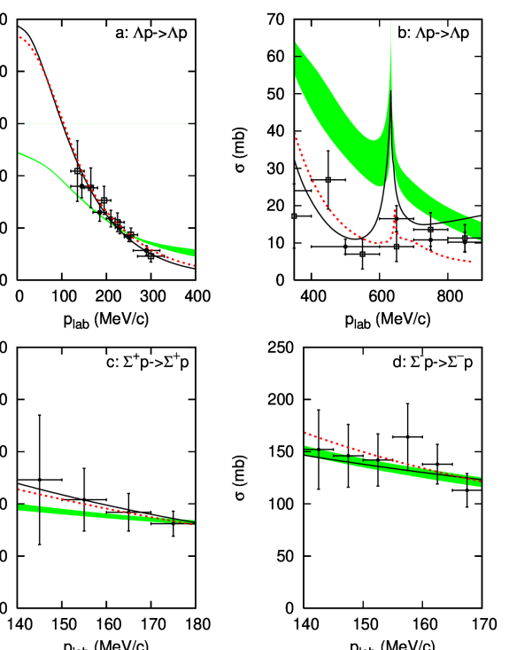
Figure 4.1: ”Total” cross section $\sigma$ (as defined in Eq. (3.2)) as a function of $p_{{\rm lab}}$. The experimental cross sections in $a$ are taken from Refs. [27] (open squares) and  [28] (filled circles), in $b$ from Refs. [30] (filled circles) and [31] (open squares) and in $c$,$d$ from [23]. The shaded band is the Jülich chiral EFT’06 A for $\Lambda=550,...,700$ MeV, the dashed curve is the Jülich ’04 model [19], and the solid curve is the Nijmegen NSC97f model [24].

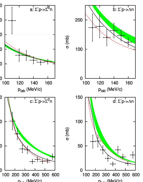
Figure 4.2: As in Figure 4.1, but now the experimental cross sections in $a$,$b$ are taken from Refs. [29] and in $c$,$d$ from [32].

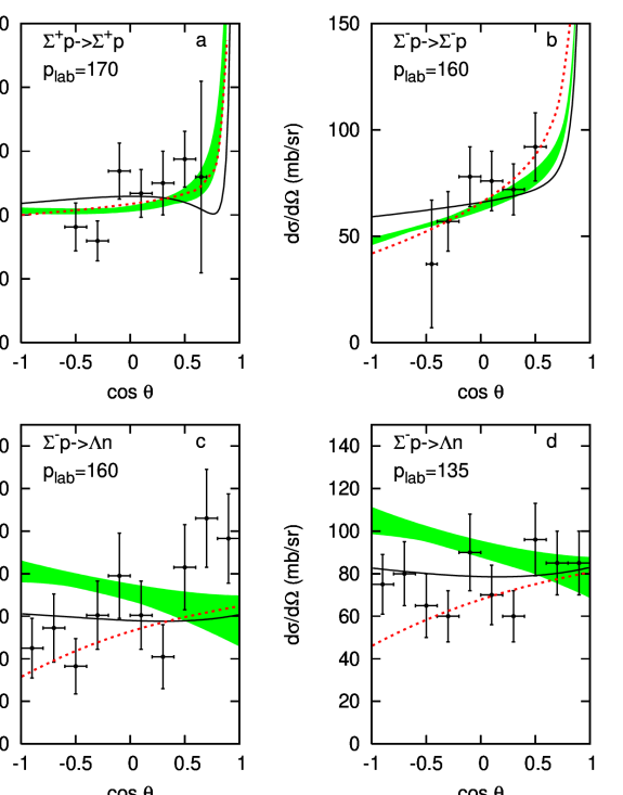
Figure 4.3: Differential cross section $d\sigma/d\cos\theta$ as a function of $\cos\theta$, where $\theta$ is the c.m. scattering angle, at various values of $p_{{\rm lab}}$ (MeV/c). The experimental differential cross sections in $a$,$b$ are taken from [23] and in $c$,$d$ from [29]. Same description of curves as in Figure 4.1.

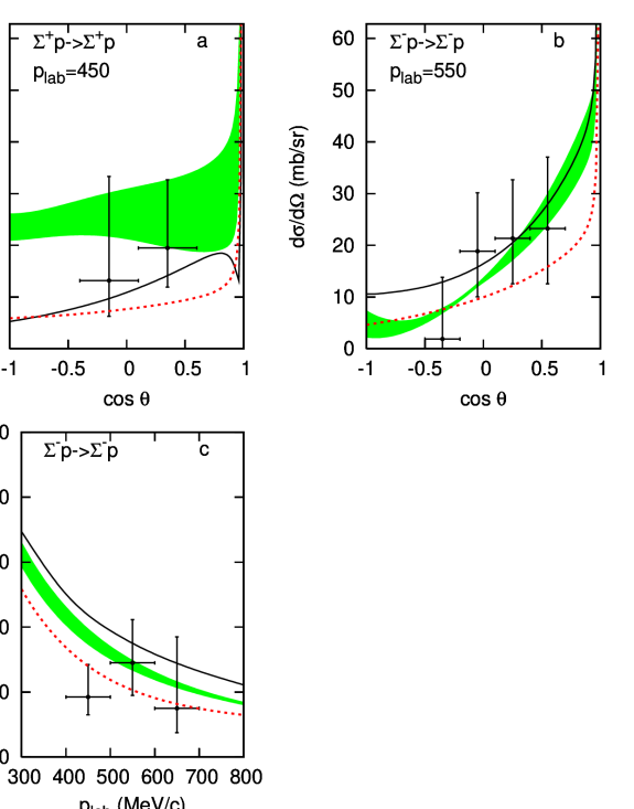
Figure 4.4: Recent $YN$ data. $a$ and $b$: differential cross section $d\sigma/d\cos\theta$ as a function of $\cos\theta$, where $\theta$ is the c.m. scattering angle, at various values of $p_{{\rm lab}}$ (MeV/c). The experimental differential cross sections are from [33] and [34], respectively. $c$: ”total” cross section $\sigma$ as a function of $p_{{\rm lab}}$. The experimental cross sections are from [34]. Same description of curves as in Figure 4.1.

In these figures the shaded band represents the results of the chiral EFT in the considered cut–off region. In this low-energy regime the cross sections are mainly given by the $S$-wave contribution, except for for the $\Lambda N\rightarrow\Sigma N$ cross section where the ${}^{3}D_{1}(\Lambda N)\leftrightarrow{}^{3}S_{1}(\Sigma N)$ transition provides the main contribution. Still all partial waves with total angular momentum $J\leq 2$ were included in the computation of the observables. The $\Lambda p$ cross section shows a clear cusp, peaking at 65 mb, at the $\Sigma^{+}n$ threshold, see Figure 4.1b. It is hard to see this effect in the experimental data, since it occurs over a very narrow energy range. Figure 4.1b shows that the predicted $\Lambda p$ cross section at higher energies is too large, which is related to the problem that some LO partial waves are too large at higher energies. Note that this was also the case for the $NN$ interaction [15]. In a NLO calculation this problem will probably vanish. The differential cross sections at low energies, which have not been taken into account in the fitting procedure, are predicted well, see Figure 4.3. The results of the chiral EFT are also in good agreement with the scattering data at higher energy, the older ones in Figures 4.2c,d as well as the more recent scattering data in Figure 4.4.

The $\Lambda p$ and $\Sigma^{+}p$ scattering lengths and effective ranges are listed in Table 4.3 together with the corresponding hypertriton binding energies (preliminary results of $YNN$ Faddeev calculations from [35]).

Table 4.3: The $YN$ singlet and triplet scattering lengths and effective ranges (in fm) and the hypertriton binding energy, $E_{B}$ (in MeV). We notice that the deuteron binding energy is $-2.224$ MeV. The binding energies for the hypertriton (last row), [35], are calculated using the Idaho-N3LO $NN$ potential [6]. The experimental value of the hypertriton binding energy is $-2.354(50)$ MeV.

$\Lambda$	550	600	650	700
$a^{\Lambda p}_{s}$	$-1.80$	$-1.80$	$-1.80$	$-1.80$
$r^{\Lambda p}_{s}$	$1.72$	$1.76$	$1.74$	$1.73$
$a^{\Lambda p}_{t}$	$-1.22$	$-1.23$	$-1.23$	$-1.23$
$r^{\Lambda p}_{t}$	$2.05$	$2.16$	$2.23$	$2.29$
$a^{\Sigma^{+}p}_{s}$	$-2.92$	$-2.26$	$-2.48$	$-2.55$
$r^{\Sigma^{+}p}_{s}$	$2.80$	$3.51$	$3.21$	$3.12$
$a^{\Sigma^{+}p}_{t}$	$0.27$	$0.65$	$0.49$	$0.46$
$r^{\Sigma^{+}p}_{t}$	$-20.37$	$-2.46$	$-5.23$	$-6.38$
$E_{B}$	$-2.272$	$-2.356$	$-2.357$	$-2.370$

The magnitudes of the $\Lambda p$ singlet and triplet scattering lengths are smaller than the corresponding values of the Nijmegen NSC97e,f and Jülich ’04 models [19, 24], which is also reflected in the small $\Lambda p$ cross section near threshold, see Figure 4.1a. The mentioned models lead to a bound hypertriton [35, 36]. Although our $\Lambda p$ scattering lengths differ significantly from those of [19, 24], the $YN$ interaction based on chiral EFT also yields a correctly bound hypertriton, see Table 4.3. Our singlet $\Sigma^{+}p$ scattering length is about half as large as the values found for the $YN$ potentials in [19, 24]. Similar to those models and other $YN$ interactions, the value of the triplet $\Sigma^{+}p$ scattering length is rather small. Contrary to [24], but similar to [19] we found repulsion in this partial wave.

The $S$- and $P$-wave phase shifts for $\Lambda p$ and $\Sigma^{+}p$ are shown in Figures 4.5 – 4.8. The shaded band represents the chiral EFT in the cut–off region $\Lambda=550,...,700$ MeV. As mentioned before, the limited accuracy of the $YN$ scattering data does not allow for a unique phase shift analysis. This explains why the chiral EFT phase shifts are quite different from the phase shifts of the models presented in Refs. [19, 24]. Actually, the predictions of the latter models also differ between each other in many partial waves. In both the $\Lambda p$ and $\Sigma^{+}p$ ${}^{1}S_{0}$ and ${}^{3}P_{0}$ partial waves, the LO chiral EFT phase shifts are much larger at higher energies than the phases from [19, 24]. We emphasize that the empirical data, considered in the fitting procedure, are at lower energies. Also for the $NN$ interaction in leading order these partial waves were much larger than the Nijmegen phase shift analysis, see [15]. It is expected that this problem for the $YN$ interaction can be solved by the derivative contact terms in a NLO calculation, just like in the $NN$ case. Our ${}^{3}S_{1}$ $\Sigma^{+}p$ phase shift is repulsive like in [19], but contrary to [24]. We remark that the $P$-waves are the result of pseudoscalar meson exchange only, since we only have contact terms in the $S$-waves. Contrary to [19], there are no spin singlet to spin triplet transitions in the chiral EFT, because of the potential form in Eq. (2.37). Although the ${}^{3}D_{1}$ $\Lambda p$ phase shift near the $\Sigma N$ threshold rises quickly, it does not go through 90 degrees like in [24]. The opening of the $\Sigma N$ channel is also clearly seen in the ${}^{3}S_{1}$ $\Lambda p$ partial wave.

We have, so far, used the $SU(6)$ value for the pseudoscalar $F/(F+D)$ ratio; $\alpha=0.4$. We studied the dependence on this parameter by varying it within a range of 10 percent; after refitting the contact terms we basically found an equally good description of the empirical data. Therefore, we keep $\alpha$ to its $SU(6)$ value. As mentioned before, at NLO one also has to consider symmetry breaking in the decay constants.

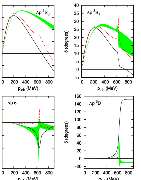
Figure 4.5: The $\Lambda p$ $S$-wave phase shifts $\delta$ as a function of $p_{{\rm lab}}$. The shaded band is the Jülich chiral EFT’06 A for $\Lambda=550,...,700$ MeV, the dashed curve is the Jülich ’04 model [19], and the solid curve is the Nijmegen NSC97f model [24]. The Nijmegen $\epsilon_{1}$ phase shown here has an other sign convention than in Ref. [24]. Since the phases of the Jülich ’04 model are calculated in the isospin basis, their $\Sigma N$ threshold does not coincide with ours.

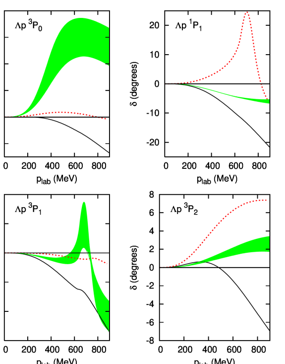
Figure 4.6: As in Figure 4.5, but now for the $P$-wave phase shifts.

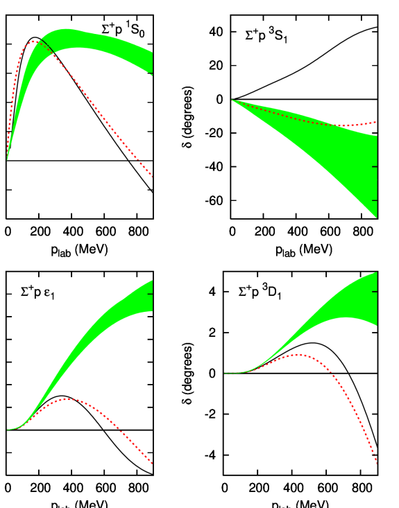
Figure 4.7: As in Figure 4.5, but now for the $\Sigma^{+}p$ $S$-wave phase shifts.

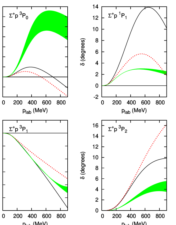
Figure 4.8: As in Figure 4.5, but now for the $\Sigma^{+}p$ $P$-wave phase shifts.

5 Summary and outlook

In this paper we have studied the $YN$ interactions in a chiral effective field theory approach based on a modified Weinberg power counting, analogous to the $NN$ case in [5]. The symmetries of QCD are explicitly incorporated. We assume that the $YN$ interactions are related via ${\rm SU(3)}_{f}$ symmetry. In principle the $YN$ interactions are also related to the $NN$ interaction via ${\rm SU(3)}_{f}$ symmetry. However, since we have done our study in leading order, in which the $NN$ interaction can not be described, we do not consider the latter, but focus on the $YN$ interactions only.

The LO potential consists of two pieces: firstly, the longer-ranged one-pseudoscalar-meson exchanges, related via ${\rm SU(3)}_{f}$ symmetry in the well-known way and secondly, the shorter ranged four-baryon contact terms without derivatives. We have derived the ${\rm SU(3)}_{f}$ invariant four-baryon contact interaction. It contains five independent contact terms that need to be determined from the empirical data. Contrary to the $NN$ case, the contact terms do not simply enter one specific partial wave because of the coupled particle channels and their ${\rm SU(3)}_{f}$ relations. Furthermore, a unique partial wave analysis for the $YN$ interaction does not exist, because of the scarce and inaccurate scattering data. Therefore we have directly fitted the parameters of the chiral EFT to the scattering observables.

The Lippmann-Schwinger equation for the LO chiral potential is solved in the partial wave basis. We have briefly discussed some details and have given the most general expressions for the $YN$ partial wave potentials in terms of the spinor invariants. The potential becomes unphysical for large momentum and has to be regularized. For this purpose we have multiplied the strong potential with an exponential regulator function. We used a cut–off in the range between $550$ and $700$ MeV. In order to incorporate the correct physical thresholds and the Coulomb interaction in the charged channels, we solve the Lippmann-Schwinger equation in the particle basis. The strong potential is, however, calculated in the isospin basis.

We have fitted the LO chiral EFT, with 5 free parameters, to 35 low-energy $YN$ scattering data. We obtained a good description of the empirical data, we found a total $\chi^{2}$ in the range between $27.8$ and $42.8$ for a cut–off in the range between $550$ and $700$ MeV. Also low-energy differential cross sections and higher energy cross sections, that were not included in the fitting procedure, were predicted quite well. Furthermore, the contact terms (found in the parameter search) are of natural size. As expected, in view of the inaccurate scattering data, the phase shifts we found differ from those found obtained for conventional boson-exchange models. We remark that in LO only the $S$-waves contain contact terms, the other partial waves are parameter free. The ${}^{1}S_{0}$ and ${}^{3}P_{0}$ partial waves are too large at higher energies, this was also a problem in the LO $NN$ study [15]. Probably this shortcoming will not occur in a NLO study, where derivative four-body contact terms may solve this problem.

We found that the chiral EFT yields a correctly bound hypertriton [35]. We did not explicitly include the hypertriton binding energy in the fitting procedure, but we have fixed the relative strength of the $\Lambda N$ singlet and triplet $S$-waves in such a way that a bound hypertriton could be obtained. We found that a $\Lambda p$ singlet scattering length of $-1.8$ fm leads to the correct binding energy.

Our findings show that the chiral effective field theory scheme, applied in Ref. [5] to the $NN$ interaction, also works well for the $YN$ interaction. In the future it will be interesting to study the convergence of the chiral EFT for the $YN$ interaction by doing NLO and NNLO calculations. In view of hypernucleus calculations, three baryon forces that naturally arise in chiral EFT, should be investigated too. Also a combined $NN$ and $YN$ study in chiral EFT, starting with a NLO calculation, needs to be performed. Work in this direction is in progress.

Appendix A Fierz theorem

Given the elements of the Clifford algebra, which are $4\times 4$-matrices,

$$\Gamma_{1}=1~{},~{}~{}\Gamma_{2}=\gamma^{\mu}~{},~{}~{}\Gamma_{3}=\sigma^{\mu\nu}~{},~{}~{}\Gamma_{4}=\gamma^{\mu}\gamma_{5}~{},~{}~{}\Gamma_{5}=\gamma_{5}~{},$$ (A.1)

the Fierz theorem [37] tells us that

$$\sum_{i}\ C_{i}\left(\Gamma_{i}\right)_{ab}\left(\Gamma_{i}\right)_{cd}=\sum_{k}\ \tilde{C}_{k}\left(\Gamma_{k}\right)_{ad}\left(\Gamma_{k}\right)_{cb}\ ,$$ (A.2)

where the new coefficients $\tilde{C}_{k}$ are related to the old coefficients $C_{i}$ by

$$\left(\begin{array}[]{l}\tilde{C}_{1}\\ \tilde{C}_{2}\\ \tilde{C}_{3}\\ \tilde{C}_{4}\\ \tilde{C}_{5}\\ \end{array}\right) = \frac{1}{4}\left(\begin{array}[]{rrrrr}1&4&12&-4&1\\ 1&-2&0&-2&-1\\ \frac{1}{2}&0&-2&0&\frac{1}{2}\\ -1&-2&0&-2&1\\ 1&-4&12&4&1\end{array}\right)\left(\begin{array}[]{l}C_{1}\\ C_{2}\\ C_{3}\\ C_{4}\\ C_{5}\end{array}\right)\ .$$ (A.18)

Appendix B Partial wave projection

Because of rotational invariance and parity conservation, the potential can be expanded into the following set of 8 spinor invariants, see for example [38, 39]. Introducing

$${\bf q}=\frac{1}{2}({\bf p}_{f}+{\bf p}_{i})\ ,\ {\bf k}={\bf p}_{f}-{\bf p}_{i}\ ,\ {\bf n}={\bf p}_{i}\times{\bf p}_{f}\ ,$$ (B.1)

we choose for the operators $P_{i}$ in spin-space

$$\begin{array}[]{ll}P_{1}=1\ ,&P_{2}=\mbox{\boldmath$\sigma$}_{1}\cdot\mbox{\boldmath$\sigma$}_{2}\ ,\\[5.69046pt] P_{3}=(\mbox{\boldmath$\sigma$}_{1}\cdot{\bf k})(\mbox{\boldmath$\sigma$}_{2}\cdot{\bf k})-\frac{1}{3}(\mbox{\boldmath$\sigma$}_{1}\cdot\mbox{\boldmath$\sigma$}_{2}){\bf k}^{2}\ ,&P_{4}=\frac{i}{2}(\mbox{\boldmath$\sigma$}_{1}+\mbox{\boldmath$\sigma$}_{2})\cdot{\bf n}\ ,\\[5.69046pt] P_{5}=(\mbox{\boldmath$\sigma$}_{1}\cdot{\bf n})(\mbox{\boldmath$\sigma$}_{2}\cdot{\bf n})\ ,&P_{6}=\frac{i}{2}(\mbox{\boldmath$\sigma$}_{1}-\mbox{\boldmath$\sigma$}_{2})\cdot{\bf n}\ ,\\[5.69046pt] \lx@intercol P_{7}=(\mbox{\boldmath$\sigma$}_{1}\cdot{\bf q})(\mbox{\boldmath$\sigma$}_{2}\cdot{\bf k})+(\mbox{\boldmath$\sigma$}_{1}\cdot{\bf k})(\mbox{\boldmath$\sigma$}_{2}\cdot{\bf q})\ ,\hfil\lx@intercol\\[5.69046pt] \lx@intercol P_{8}=(\mbox{\boldmath$\sigma$}_{1}\cdot{\bf q})(\mbox{\boldmath$\sigma$}_{2}\cdot{\bf k})-(\mbox{\boldmath$\sigma$}_{1}\cdot{\bf k})(\mbox{\boldmath$\sigma$}_{2}\cdot{\bf q})\ .\hfil\lx@intercol\end{array}$$ (B.2)

Here we follow [39], where in contrast to [40], we have chosen $P_{3}$ to be a purely ‘tensor-force’ operator. The operators $P_{3}$, $P_{5}$ and $P_{7}$ give rise to triplet coupled states (${}^{3}S_{1}\leftrightarrow{}^{3}D_{1}$, etc.). The operators $P_{6}$ and $P_{8}$ give spin singlet-triplet transitions (${}^{1}P_{1}\leftrightarrow{}^{3}P_{1}$, etc.). The expansion of the potential in spinor-invariants reads

$$V({\bf p}_{f},{\bf p}_{i})=\sum_{i=1}^{8}\ V^{(i)}({\bf p}_{f},{\bf p}_{i})\ P_{i}({\bf p}_{f},{\bf p}_{i})\ .$$ (B.3)

We will use the following shorthand notation for the potentials in the LSJ basis for the two parity ($P$) classes:
(i) $P=(-)^{J}$:

$$V^{J}_{0,0}=\left(J0J\left|V\right|J0J\right) \hskip 14.22636pt,\hskip 14.22636pt V^{J}_{0,2}=\left(J0J\left|V\right|J1J\right)\ ,$$

$$V^{J}_{2,0}=\left(J1J\left|V\right|J0J\right) \hskip 14.22636pt,\hskip 14.22636pt V^{J}_{2,2}=\left(J1J\left|V\right|J1J\right)\ .$$ (B.4)

(ii) $P=-(-)^{J}$:

$$V^{J}_{1,1}=\left(J-1,1J\left|V\right|J-1,1J\right) \hskip 7.11317pt,\hskip 7.11317pt V^{J}_{1,3}=\left(J-1,1J\left|V\right|J+1,1J\right)\ ,$$

$$V^{J}_{3,1}=\left(J+1,1J\left|V\right|J-1,1J\right) \hskip 7.11317pt,\hskip 7.11317pt V^{J}_{3,3}=\left(J+1,1J\left|V\right|J+1,1J\right)\ ,$$ (B.5)

where it is always understood that the final and initial state momenta are $p_{f}$ and $p_{i}$ respectively, e.g. $V^{J}_{0,0}=V^{J}_{0,0}(p_{f},p_{i})$ etc. Using the nomenclature $V_{J}^{(1)}=V_{J}^{(C)}$ for the central potential, $V_{J}^{(2)}=V_{J}^{(\sigma)}$ for the spin–spin potential, $V_{J}^{(3)}=V_{J}^{(T)}$ for the tensor potential, $V_{J}^{(4)}=V_{J}^{(SO)}$ for the spin–orbit potential, $V_{J}^{(5)}=V_{J}^{(Q)}$ for the quadratic spin–orbit potential and $V_{J}^{(6)}=V_{J}^{(ASO)}$ for the antisymmetric spin–orbit potential, the following partial wave potentials are found for $J>0$.

$$V^{J}_{0,0} = 4\pi\left[V_{J}^{(C)}-3V_{J}^{(\sigma)}+p_{f}^{2}p_{i}^{2}\left(e_{0,0}^{(5,+)}V_{J-2}^{(Q)}+f_{0,0}^{(5,+)}V_{J}^{(Q)}+g_{0,0}^{(5,+)}V_{J+2}^{(Q)}\right)\right.$$

$$\left.+\left(p_{f}^{2}+p_{i}^{2}\right)\cos 2\psi\ V_{J}^{(7)}\right]\ ,$$

$$V^{J}_{0,2} = 4\pi\frac{\sqrt{J(J+1)}}{2J+1}\left[p_{f}p_{i}\left(V_{J-1}^{(ASO)}-V_{J+1}^{(ASO)}\right)+2p_{f}p_{i}\left(V_{J-1}^{(8)}-V_{J+1}^{(8)}\right)\right]\ ,$$

$$V^{J}_{2,0} = 4\pi\frac{\sqrt{J(J+1)}}{2J+1}\left[p_{f}p_{i}\left(V_{J-1}^{(ASO)}-V_{J+1}^{(ASO)}\right)-2p_{f}p_{i}\left(V_{J-1}^{(8)}-V_{J+1}^{(8)}\right)\right]\ ,$$

$$V^{J}_{2,2} = 4\pi\left[V_{J}^{(C)}+V_{J}^{(\sigma)}+\frac{2}{3}\left(p_{f}^{2}+p_{i}^{2}\right)\left(V_{J}^{(T)}-\frac{1}{2}\sin 2\psi\ \left\{\frac{2J+3}{2J+1}V_{J-1}^{(T)}+\frac{2J-1}{2J+1}V_{J+1}^{(T)}\right\}\right)\right.$$

$$\left.-p_{f}p_{i}\frac{1}{2J+1}\left(V_{J-1}^{(SO)}-V_{J+1}^{(SO)}\right)+p_{f}^{2}p_{i}^{2}\left(e_{1,1}^{(5,+)}V_{J-2}^{(Q)}+f_{1,1}^{(5,+)}V_{J}^{(Q)}+g_{1,1}^{(5,+)}V_{J+2}^{(Q)}\right)\right.$$

$$\left.-\left(p_{f}^{2}+p_{i}^{2}\right)\cos 2\psi\ V_{J}^{(7)}\right]\ ,$$

$$V^{J}_{1,1} = 4\pi\left[V_{J-1}^{(C)}+V_{J-1}^{(\sigma)}+\frac{2}{3}\left(p_{f}^{2}+p_{i}^{2}\right)\frac{J-1}{2J+1}\left(-V_{J-1}^{(T)}+\frac{1}{2}\sin 2\psi\ \left\{\frac{2J-3}{2J-1}V_{J}^{(T)}+\right.\right.\right.$$

$$\left.\left.\left.\frac{2J+1}{2J-1}V_{J-2}^{(T)}\right\}\right)+p_{f}p_{i}\frac{J-1}{2J-1}\left(V_{J-2}^{(SO)}-V_{J}^{(SO)}\right)+p_{f}^{2}p_{i}^{2}\left(e_{J-1,J-1}^{(5,-)}V_{J-3}^{(Q)}+\right.\right.$$

$$\left.\left.f_{J-1,J-1}^{(5,-)}V_{J-1}^{(Q)}+g_{J-1,J-1}^{(5,-)}V_{J+1}^{(Q)}\right)-\left(p_{f}^{2}+p_{i}^{2}\right)\cos 2\psi\ \frac{1}{2J+1}V_{J-1}^{(7)}\right]\ ,$$

$$V^{J}_{1,3} = 4\pi\left[2\left(p_{f}^{2}+p_{i}^{2}\right)\frac{\sqrt{J(J+1)}}{2J+1}\left(\sin 2\psi\ V_{J}^{(T)}-\left\{\cos^{2}\psi\ V_{J-1}^{(T)}+\sin^{2}\psi\ V_{J+1}^{(T)}\right\}\right)\right.$$

$$\left.-p_{f}^{2}p_{i}^{2}f_{J+1,J-1}^{(5,-)}\left(V_{J+1}^{(Q)}-V_{J-1}^{Q)}\right)+\left(p_{f}^{2}+p_{i}^{2}\right)\frac{2\sqrt{J(J+1)}}{2J+1}\left(-\sin^{2}\psi\ V_{J+1}^{(7)}+\right.\right.$$

$$\left.\left.\cos^{2}\psi\ V_{J-1}^{(7)}\right)\vphantom{\frac{\sqrt{J(J+1)}}{2J+1}}\right]\ ,$$

$$V^{J}_{3,1} = 4\pi\left[2\left(p_{f}^{2}+p_{i}^{2}\right)\frac{\sqrt{J(J+1)}}{2J+1}\left(\sin 2\psi\ V_{J}^{(T)}-\left\{\cos^{2}\psi\ V_{J+1}^{(T)}+\sin^{2}\psi\ V_{J-1}^{(T)}\right\}\right)\right.$$

$$\left.-p_{f}^{2}p_{i}^{2}f_{J+1,J-1}^{(5,-)}\left(V_{J+1}^{(Q)}-V_{J-1}^{Q)}\right)+\left(p_{f}^{2}+p_{i}^{2}\right)\frac{2\sqrt{J(J+1)}}{2J+1}\left(-\sin^{2}\psi\ V_{J-1}^{(7)}+\right.\right.$$

$$\left.\left.\cos^{2}\psi\ V_{J+1}^{(7)}\right)\vphantom{\frac{\sqrt{J(J+1)}}{2J+1}}\right]\ ,$$

$$V^{J}_{3,3} = 4\pi\left[V_{J+1}^{(C)}+V_{J+1}^{(\sigma)}+\frac{2}{3}\left(p_{f}^{2}+p_{i}^{2}\right)\frac{J+2}{2J+1}\left(-V_{J+1}^{(T)}+\frac{1}{2}\sin 2\psi\ \left\{\frac{2J+5}{2J+3}V_{J}^{(T)}+\right.\right.\right.$$ (B.6)

$$\left.\left.\left.\frac{2J+1}{2J+3}V_{J+2}^{(T)}\right\}\right)-p_{f}p_{i}\frac{J+2}{2J+3}\left(V_{J}^{(SO)}-V_{J+2}^{(SO)}\right)+p_{f}^{2}p_{i}^{2}\left(e_{J+1,J+1}^{(5,-)}V_{J-1}^{(Q)}+\right.\right.$$

$$\left.\left.f_{J+1,J+1}^{(5,-)}V_{J+1}^{(Q)}+g_{J+1,J+1}^{(5,-)}V_{J+3}^{(Q)}\right)+\left(p_{f}^{2}+p_{i}^{2}\right)\cos 2\psi\ \frac{1}{2J+1}V_{J+1}^{(7)}\right]\ .$$

For $J=0$ the two non-zero partial wave potentials are

$$V^{J}_{0,0} = 4\pi\left[V_{0}^{(C)}-3V_{0}^{(\sigma)}+\frac{2}{3}p_{f}^{2}p_{i}^{2}\left(-V_{0}^{(Q)}+V_{2}^{(Q)}\right)+\left(p_{f}^{2}+p_{i}^{2}\right)\cos 2\psi\ V_{0}^{(7)}\right]\ ,$$

$$V^{J}_{3,3} = 4\pi\left[V_{1}^{(C)}+V_{1}^{(\sigma)}+\frac{4}{3}\left(p_{f}^{2}+p_{i}^{2}\right)\left(-V_{1}^{(T)}+\frac{1}{2}\sin 2\psi\ \left\{\frac{5}{3}V_{0}^{(T)}+\frac{1}{3}V_{2}^{(T)}\right\}\right)\right.$$ (B.7)

$$\left.-p_{f}p_{i}\frac{2}{3}\left(V_{0}^{(SO)}-V_{2}^{(SO)}\right)+\frac{2}{5}p_{f}^{2}p_{i}^{2}\left(V_{1}^{(Q)}-V_{3}^{(Q)}\right)\right.$$

$$\left.+\left(p_{f}^{2}+p_{i}^{2}\right)\cos 2\psi\ V_{1}^{(7)}\vphantom{\frac{5}{3}}\right]\ .$$

In the formulae above we have used

$$V^{(i)}_{J}(p_{f},p_{i}) = \frac{1}{2}\int_{-1}^{1}d\cos\theta\ V^{(i)}({\bf p}_{f},{\bf p}_{i})P_{J}(\cos\theta)\ .$$ (B.8)

Details of the derivation and definitions of $\cos 2\psi$, $\sin 2\psi$ and the various $e^{(5)}$, $f^{(5)}$ and $g^{(5)}$ factors can be found in Appendix C. We note that an additional overall (-) sign for the off-diagonal $V^{J}_{1,3}$ and $V^{J}_{3,1}$ has been used in the calculations.

Appendix C Partial wave projection of spinor invariants

With the matrix elements for the spinor invariants in this appendix (found using the results of Appendix C.1), the partial wave potentials in Appendix B can be readily derived. The derivation in this appendix is an extension of the derivation for the $NN$ case in [41].

Distinguishing between the partial waves with parity $P=(-)^{J}$ and $P=-(-)^{J}$, we write the potential matrix elements on the LSJ-basis in the following way (see e.g. [38]):
(i) $P=(-)^{J}$:

$$(p_{f};L^{\prime}S^{\prime}J^{\prime}M^{\prime}|\ V\ |p_{i};LSJM)=4\pi\,\delta_{J^{\prime}J}\ \delta_{M^{\prime}M}\ \delta_{L^{\prime}L}\,V^{J,+}(S^{\prime},S)\ .$$ (C.9)

(ii) $P=-(-)^{J}$:

$$(p_{f};L^{\prime}S^{\prime}J^{\prime}M^{\prime}|\ V\ |p_{i};LSJM)=4\pi\,\delta_{J^{\prime}J}\,\delta_{M^{\prime}M}\,\delta_{S^{\prime}S}\,V^{J,-}(L^{\prime},L)\ .$$ (C.10)

For notational convenience we will use as an index the parity factor $\eta$, which is defined by writing $P=\eta(-)^{J}$. The $P=(-)^{J}$ states contain the spin singlet and triplet-uncoupled states ($\eta=+$), and the $P=-(-)^{J}$ states contain the spin triplet-coupled states ($\eta=-$).

Below we list the partial wave matrix elements for $\eta=\pm$ for the different $V^{(i)}\ P_{i},(i=1,...,8)$. Here we restrict ourselves to the matrix elements $\neq 0$.
1. central $P_{1}=1$:

$$(p_{f};L^{\prime}S^{\prime}J^{\prime}M^{\prime}|V^{(1)}P_{1}|p_{i};LSJM) = 4\pi\,\delta_{J^{\prime}J}\,\delta_{M^{\prime}M}\,F^{J,\eta}_{1}(L^{\prime}\ S^{\prime},L\ S)\ ,$$ (C.11)

$${\rm with}\hskip 14.22636ptF^{J,\eta}_{1}(L^{\prime}\ S^{\prime},L\ S)\ = \delta_{L^{\prime}L}\,\delta_{S^{\prime}S}\,V^{(1)}_{L}\ .$$

2. spin-spin $P_{2}=\mbox{\boldmath$\sigma$}_{1}\cdot\mbox{\boldmath$\sigma$}_{2}$:

$$(p_{f};L^{\prime}S^{\prime}J^{\prime}M^{\prime}|V^{(2)}P_{2}|p_{i};LSJM) = 4\pi\,\delta_{J^{\prime}J}\,\delta_{M^{\prime}M}\,F^{J,\eta}_{2}(L^{\prime}\ S^{\prime},L\ S)\ ,$$ (C.12)

$${\rm with}\hskip 14.22636ptF^{J,\eta}_{2}(L^{\prime}\ S^{\prime},L\ S)\ = \delta_{L^{\prime}L}\,\delta_{S^{\prime}S}\,\left[2S(S+1)-3\right]V^{(2)}_{L}\ .$$

3. tensor $P_{3}=(\mbox{\boldmath$\sigma$}_{1}\cdot{\bf k})(\mbox{\boldmath$\sigma$}_{2}\cdot{\bf k})-\frac{1}{3}(\mbox{\boldmath$\sigma$}_{1}\cdot\mbox{\boldmath$\sigma$}_{2}){\bf k}^{2}$:

$$(p_{f};L^{\prime}S^{\prime}J^{\prime}M^{\prime}|V^{(3)}P_{3}|p_{i};LSJM)=\frac{8\pi}{3}(p_{f}^{2}+p_{i}^{2})\,\delta_{J^{\prime}J}\,\delta_{M^{\prime}M}\,F^{J,\eta}_{3}(i,j)\ ,$$ (C.13)

where $i=S^{\prime}$ and $j=S$ for $\eta=+$, respectively $i=L^{\prime}$ and $j=L$ for $\eta=-$.
(i) triplet uncoupled: $L=L^{\prime}=J,\ S=S^{\prime}=1$

$$F^{J,+}_{3}(1,1) = \left[V^{(3)}_{J}-\frac{1}{2}\sin 2\psi\left(\frac{2J+3}{2J+1}V^{(3)}_{J-1}+\frac{2J-1}{2J+1}V^{(3)}_{J+1}\right)\right]\ .$$ (C.14)

(ii) triplet coupled: $L=J\pm 1,\ L^{\prime}=J\pm 1,\ S=S^{\prime}=1$

$$F^{J,-}_{3}(J-1,J-1) = \frac{J-1}{2J+1}\ \left[-V^{(3)}_{J-1}+\frac{1}{2}\sin 2\psi\left(\frac{2J-3}{2J-1}V^{(3)}_{J}+\frac{2J+1}{2J-1}V^{(3)}_{J-2}\right)\right]\ ,$$

$$F^{J,-}_{3}(J-1,J+1) = -3\frac{\sqrt{J(J+1)}}{2J+1}\ \left[-\sin 2\psi\ V^{(3)}_{J}+\left(\cos^{2}\psi V^{(3)}_{J-1}+\sin^{2}\psi V^{(3)}_{J+1}\right)\right]\ ,$$

$$F^{J,-}_{3}(J+1,J-1) = -3\frac{\sqrt{J(J+1)}}{2J+1}\ \left[-\sin 2\psi\ V^{(3)}_{J}+\left(\sin^{2}\psi V^{(3)}_{J-1}+\cos^{2}\psi V^{(3)}_{J+1}\right)\right]\ ,$$

$$F^{J,-}_{3}(J+1,J+1) = \frac{J+2}{2J+1}\ \left[-V^{(3)}_{J+1}+\frac{1}{2}\sin 2\psi\left(\frac{2J+5}{2J+3}V^{(3)}_{J}+\frac{2J+1}{2J+3}V^{(3)}_{J+2}\right)\right]\ ,$$ (C.15)

where we introduced

$$\cos\psi=\frac{p_{i}}{\sqrt{p_{f}^{2}+p_{i}^{2}}}\hskip 14.22636pt,\hskip 14.22636pt\sin\psi=\frac{p_{f}}{\sqrt{p_{f}^{2}+p_{i}^{2}}}\ .$$ (C.16)

4. spin-orbit $P_{4}=\frac{i}{2}(\mbox{\boldmath$\sigma$}_{1}+\mbox{\boldmath$\sigma$}_{2})\cdot{\bf n}$:

$$(p_{f};L^{\prime}S^{\prime}J^{\prime}M^{\prime}|V^{(4)}P_{4}|p_{i};LSJM) = 4\pi\,p_{f}p_{i}\delta_{J^{\prime}J}\,\delta_{M^{\prime}M}\,F^{J,\eta}_{4}(i,j)\ .$$ (C.17)

(i) triplet uncoupled: $L=L^{\prime}=J,\ S=S^{\prime}=1$

$$F^{J,+}_{4}(1,1)=-\left(V^{(4)}_{J-1}-V^{(4)}_{J+1}\right)/(2J+1)\ .$$ (C.18)

(ii) triplet coupled: $L=J\pm 1,\ L^{\prime}=J\pm 1,\ S=S^{\prime}=1$

$$F^{J,-}_{4}(J-1,J-1) = \hskip 8.5359pt\frac{(J-1)}{(2J-1)}\left(V^{(4)}_{J-2}-V^{(4)}_{J}\right)\ ,$$

$$F^{J,-}_{4}(J+1,J+1) = -\frac{(J+2)}{(2J+3)}\left(V^{(4)}_{J}-V^{(4)}_{J+2}\right)\ .$$ (C.19)

5. quadratic-spin-orbit $P_{5}=(\mbox{\boldmath$\sigma$}_{1}\cdot{\bf n})(\mbox{\boldmath$\sigma$}_{2}\cdot{\bf n})$:

$$(p_{f};L^{\prime}S^{\prime}J^{\prime}M^{\prime}|V^{(5)}P_{5}|p_{i};LSJM)=4\pi p_{f}^{2}p_{i}^{2}\,\delta_{J^{\prime}J}\,\delta_{M^{\prime}M}\,F^{J,\eta}_{5}(i,j)\ .$$ (C.20)

(i) singlet: $L=L^{\prime}=J,\ S=S^{\prime}=0$

$$F^{J,+}_{5}(0,0) = e^{(5,+)}_{0,0}V^{(5)}_{J-2}+f^{(5,+)}_{0,0}V^{(5)}_{J}+g^{(5,+)}_{0,0}V^{(5)}_{J+2}\ .$$ (C.21)

(ii) triplet uncoupled: $L=L^{\prime}=J,\ S=S^{\prime}=1$

$$F^{J,+}_{5}(1,1) = e^{(5,+)}_{1,1}V^{(5)}_{J-2}+f^{(5,+)}_{1,1}V^{(5)}_{J}+g^{(5,+)}_{1,1}V^{(5)}_{J+2}\ ,$$ (C.22)

where we introduced

$$e^{(5,+)}_{0,0} = +\frac{J(J-1)}{(2J-1)(2J+1)}\hskip 14.22636pt,\hskip 14.22636pte^{(5,+)}_{1,1}=+\frac{(J-1)(J+2)}{(2J-1)(2J+1)}\ ,$$

$$f^{(5,+)}_{0,0} = -\frac{2(J^{2}+J-1)}{(2J-1)(2J+3)}\hskip 14.22636pt,\hskip 14.22636ptf^{(5,+)}_{1,1}=-\frac{2(J-1)(J+2)}{(2J-1)(2J+3)}\ ,$$

$$g^{(5,+)}_{0,0} = +\frac{(J+1)(J+2)}{(2J+1)(2J+3)}\hskip 14.22636pt,\hskip 14.22636ptg^{(5,+)}_{1,1}=+\frac{(J-1)(J+2)}{(2J+1)(2J+3)}\ .$$ (C.23)

(iii) triplet coupled: $L=J\pm 1,\ L^{\prime}=J\pm 1,\ S=S^{\prime}=1$

$$F^{J,-}_{5}(J-1,J-1) = e^{(5,-)}_{J-1,J-1}V^{(5)}_{J-3}+f^{(5,-)}_{J-1,J-1}V^{(5)}_{J-1}+g^{(5,-)}_{J-1,J-1}V^{(5)}_{J+1}\ ,$$

$$F^{J,-}_{5}(J\pm 1,J\mp 1) = -f^{(5,-)}_{J+1,J-1}\left[V^{(5)}_{J+1}-V^{(5)}_{J-1}\right]\ ,$$

$$F^{J,-}_{5}(J+1,J+1) = e^{(5,-)}_{J+1,J+1}V^{(5)}_{J-1}+f^{(5,-)}_{J+1,J+1}V^{(5)}_{J+1}+g^{(5,-)}_{J+1,J+1}V^{(5)}_{J+3}\ ,$$ (C.24)

where we introduced

$$e^{(5,-)}_{J-1,J-1} = -\frac{(J-1)(J-2)}{(2J-1)(2J-3)}\hskip 14.22636pt,\hskip 14.22636pte^{(5,-)}_{J+1,J+1}=-\frac{J(2J^{2}+7J+7)}{(2J+1)^{2}(2J+3)}\ ,$$

$$f^{(5,-)}_{J-1,J-1} = 2\frac{(2J^{3}-3J^{2}-2J+2)}{(2J+1)^{2}(2J-3)}\hskip 14.22636pt,\hskip 14.22636ptf^{(5,-)}_{J+1,J+1}=2\frac{(2J^{3}+9J^{2}+10J+1)}{(2J+1)^{2}(2J+5)}\ ,$$

$$g^{(5,-)}_{J-1,J-1} = -\frac{(2J^{2}-3J+2)(J+1)}{(2J+1)^{2}(2J-1)}\hskip 14.22636pt,\hskip 14.22636ptg^{(5,-)}_{J+1,J+1}=-\frac{(J+2)(J+3)}{(2J+3)(2J+5)}\ ,$$

$$f^{(5,-)}_{J+1,J-1} = 2\frac{\sqrt{J(J+1)}}{(2J+1)^{2}}\ .$$ (C.25)

6. antisymmetric spin-orbit $P_{6}=\frac{i}{2}(\mbox{\boldmath$\sigma$}_{1}-\mbox{\boldmath$\sigma$}_{2})\cdot{\bf n}$:

$$(p_{f};L^{\prime}S^{\prime}J^{\prime}M^{\prime}|V^{(6)}P_{6}|p_{i};LSJM) = 4\pi\,p_{f}p_{i}\delta_{J^{\prime}J}\,\delta_{M^{\prime}M}\,F^{J,\eta}_{6}(i,j)\ .$$ (C.26)

(i) singlet-triplet uncoupled: $L=L^{\prime}=J,\ S\neq S^{\prime}$

$$F^{J,+}_{6}(1,0)=F^{J,+}_{6}(0,1)=\frac{\sqrt{J(J+1)}}{2J+1}\left(V^{(6)}_{J-1}-V^{(6)}_{J+1}\right)\ .$$ (C.27)

7. $P_{7}=(\mbox{\boldmath$\sigma$}_{1}\cdot{\bf q})(\mbox{\boldmath$\sigma$}_{2}\cdot{\bf k})+(\mbox{\boldmath$\sigma$}_{1}\cdot{\bf k})(\mbox{\boldmath$\sigma$}_{2}\cdot{\bf q})$:

$$(p_{f};L^{\prime}S^{\prime}J^{\prime}M^{\prime}|V^{(7)}P_{7}|p_{i};LSJM)=4\pi(p_{f}^{2}+p_{i}^{2})\,\delta_{J^{\prime}J}\,\delta_{M^{\prime}M}\,F^{J,\eta}_{7}(i,j)\ .$$ (C.28)

(i) singlet: $L=L^{\prime}=J,\ S=S^{\prime}=0$

$$F^{J,+}_{7}(0,0) = \cos 2\psi\ V^{(7)}_{J}\ .$$ (C.29)

(ii) triplet uncoupled: $L=L^{\prime}=J,\ S=S^{\prime}=1$

$$F^{J,+}_{7}(1,1) = -\cos 2\psi\ V^{(7)}_{J}\ .$$ (C.30)

(iii) triplet coupled: $L=J\pm 1,\ L^{\prime}=J\pm 1,\ S=S^{\prime}=1$

$$F^{J,-}_{7}(J-1,J-1) = -\frac{1}{2J+1}\cos 2\psi\ V^{(7)}_{J-1}\ ,$$

$$F^{J,-}_{7}(J-1,J+1) = 2\frac{\sqrt{J(J+1)}}{2J+1}\ \left[-\sin^{2}\psi\ V^{(7)}_{J-1}+\cos^{2}\psi\ V^{(7)}_{J+1}\right]\ ,$$

$$F^{J,-}_{7}(J+1,J-1) = 2\frac{\sqrt{J(J+1)}}{2J+1}\ \left[-\sin^{2}\psi\ V^{(7)}_{J+1}+\cos^{2}\psi\ V^{(7)}_{J-1}\right]\ ,$$

$$F^{J,-}_{7}(J+1,J+1) = \frac{1}{2J+1}\cos 2\psi\ V^{(7)}_{J+1}\ .$$ (C.31)

8. $P_{8}=(\mbox{\boldmath$\sigma$}_{1}\cdot{\bf q})(\mbox{\boldmath$\sigma$}_{2}\cdot{\bf k})-(\mbox{\boldmath$\sigma$}_{1}\cdot{\bf k})(\mbox{\boldmath$\sigma$}_{2}\cdot{\bf q})$:

$$(p_{f};L^{\prime}S^{\prime}J^{\prime}M^{\prime}|V^{(8)}P_{8}|p_{i};LSJM) = 4\pi\,\left(p_{f}^{2}+p_{i}^{2}\right)\delta_{J^{\prime}J}\,\delta_{M^{\prime}M}\,F^{J,\eta}_{8}(i,j)\ .$$ (C.32)

(i) singlet-triplet uncoupled: $L=L^{\prime}=J,\ S\neq S^{\prime}$

$$F^{J,+}_{8}(1,0)=-F^{J,+}_{8}(0,1)=-\frac{\sqrt{J(J+1)}}{2J+1}\sin 2\psi\ \left(V^{(8)}_{J-1}-V^{(8)}_{J+1}\right)\ .$$ (C.33)

Henceforth, we will use the following shorthand notation for the potentials:
(i) $P=(-)^{J}$:

$$V^{J}_{0,0}=V^{J,+}(0,0) \hskip 14.22636pt,\hskip 14.22636pt V^{J}_{0,2}=V^{J,+}(0,1)\ ,$$

$$V^{J}_{2,0}=V^{J,+}(1,0) \hskip 14.22636pt,\hskip 14.22636pt V^{J}_{2,2}=V^{J,+}(1,1)\ .$$ (C.34)

(ii) $P=-(-)^{J}$:

$$V^{J}_{1,1}=V^{J,-}(J-1,J-1) \hskip 14.22636pt,\hskip 14.22636pt V^{J}_{1,3}=V^{J,-}(J-1,J+1)\ ,$$

$$V^{J}_{3,1}=V^{J,-}(J+1,J-1) \hskip 14.22636pt,\hskip 14.22636pt V^{J}_{3,3}=V^{J,-}(J+1,J+1)\ ,$$ (C.35)

where it is always understood that the final and initial state momenta are $p_{f}$ and $p_{i}$ respectively, e.g. $V^{J}_{0,0}=V^{J}_{0,0}(p_{f},p_{i})$ etc.

C.1 The LSJ representation operators

From the formulas given in this section the partial wave projections of the spinor invariants, as given above , can be derived in a straightforward manner.

The spherical wave functions in momentum space with quantum numbers J, L, S, are in the SYM-convention [42]

$${\mathcal{Y}}_{JLS}^{M}(\hat{\bf p})=i^{L}\ \mbox{\large\bf$C$}^{J\ L\ S}_{M\ m\ \mu}Y^{L}_{m}(\hat{\bf p})\chi^{S}_{\mu}\ ,$$ (C.1)

where $\chi$ is the two-nucleon spin wave function. Then

$$\left({\bf S}\cdot\hat{\bf p}\right){\mathcal{Y}}_{JLS}^{M}(\hat{\bf p}) = i\sqrt{6}\ \left\{\sqrt{\frac{L}{2L-1}}\left[\begin{array}[]{ccc}L&S&J\\ 1&1&0\\ L-1&S&J\end{array}\right]{\mathcal{Y}}_{JL-1S}^{M}(\hat{\bf p})\right.$$ (C.9)

$$\left.+\sqrt{\frac{L+1}{2L+3}}\left[\begin{array}[]{ccc}L&S&J\\ 1&1&0\\ L+1&S&J\end{array}\right]{\mathcal{Y}}_{JL+1S}^{M}(\hat{\bf p})\right\}\ ,$$

where ${\bf S}=\left(\mbox{\boldmath$\sigma$}_{1}+\mbox{\boldmath$\sigma$}_{2}\right)/2$. The $9j$-symbols differ from [43], formula $(6.4.4)$, in the replacement of the $3j$-symbols by the Clebsch-Gordan coefficients and by leaving out the $m_{33}$–summation. Working this out explicitly, we find

$$\left({\bf S}\cdot\hat{\bf p}\right){\mathcal{Y}}_{JJ-11}^{M}(\hat{\bf p}) = -i\ a_{J}\ {\mathcal{Y}}_{JJ1}^{M}(\hat{\bf p})\ ,$$

$$\left({\bf S}\cdot\hat{\bf p}\right){\mathcal{Y}}_{JJ+11}^{M}(\hat{\bf p}) = \hskip 8.5359pti\ b_{J}\ {\mathcal{Y}}_{JJ1}^{M}(\hat{\bf p})\ ,$$

$$\left({\bf S}\cdot\hat{\bf p}\right){\mathcal{Y}}_{J\ J\ 1}^{M}(\hat{\bf p}) = \hskip 8.5359pti\ a_{J}\ {\mathcal{Y}}_{JJ-11}^{M}(\hat{\bf p})-i\ b_{J}\ {\mathcal{Y}}_{JJ+11}^{M}(\hat{\bf p})\ ,$$ (C.11)

where

$$a_{J}=-\sqrt{\frac{J+1}{2J+1}}\hskip 28.45274pt,\hskip 28.45274ptb_{J}=-\sqrt{\frac{J}{2J+1}}\ .$$ (C.12)

Ordering the states according to $L=J-1,L=J,L=J+1$ , we can write in matrix form

$$\left(\begin{array}[]{ccc}L&=&J-1\\ &&J\\ &&J+1\end{array}\right\|{\bf S}\cdot\hat{\bf p}\left\|\begin{array}[]{ccc}L&=&J-1\\ &&J\\ &&J+1\end{array}\right)=\left(\begin{array}[]{ccc}0&ia_{J}&0\\ -ia_{J}&0&ib_{J}\\ 0&-ib_{J}&0\end{array}\right)\ .$$ (C.22)

Similarly we find for the operator ${\bf AS}=\left(\mbox{\boldmath$\sigma$}_{1}-\mbox{\boldmath$\sigma$}_{2}\right)/2$:

$$\left({\bf AS}\cdot\hat{\bf p}\right){\mathcal{Y}}_{JLS}^{M}(\hat{\bf p}) = \sum_{S^{\prime}}i\sqrt{3}\ \left\{\sqrt{\frac{L}{2L-1}}\left[\begin{array}[]{ccc}L&S&J\\ 1&1&0\\ L-1&S^{\prime}&J\end{array}\right]{\mathcal{Y}}_{JL-1S^{\prime}}^{M}(\hat{\bf p})+\right.$$ (C.30)

$$\left.\sqrt{\frac{L+1}{2L+3}}\left[\begin{array}[]{ccc}L&S&J\\ 1&1&0\\ L+1&S^{\prime}&J\end{array}\right]{\mathcal{Y}}_{JL+1S^{\prime}}^{M}(\hat{\bf p})\right\}\left\{\delta_{S^{\prime},1}\delta_{S,0}-\sqrt{3}\delta_{S^{\prime},0}\delta_{S,1}\right\}\ .$$

Working this out explicitly, we find

$$\left({\bf AS}\cdot\hat{\bf p}\right){\mathcal{Y}}_{JJ-11}^{M}(\hat{\bf p}) = i\ b_{J}\ {\mathcal{Y}}_{JJ0}^{M}(\hat{\bf p})\ ,$$

$$\left({\bf AS}\cdot\hat{\bf p}\right){\mathcal{Y}}_{JJ+11}^{M}(\hat{\bf p}) = \hskip 8.5359pti\ a_{J}\ {\mathcal{Y}}_{JJ0}^{M}(\hat{\bf p})\ ,$$

$$\left({\bf AS}\cdot\hat{\bf p}\right){\mathcal{Y}}_{J\ J\ 1}^{M}(\hat{\bf p}) = 0\ ,$$

$$\left({\bf AS}\cdot\hat{\bf p}\right){\mathcal{Y}}_{J\ J\ 0}^{M}(\hat{\bf p}) = \hskip 8.5359pt-i\ b_{J}\ {\mathcal{Y}}_{JJ-11}^{M}(\hat{\bf p})-i\ a_{J}\ {\mathcal{Y}}_{JJ+11}^{M}(\hat{\bf p})\ .$$ (C.32)

From the results above one can derive the following useful partial wave projections. For the spin triplet states:

$$(L^{\prime}1J|V({\bf k}^{2})\left({\bf S}\cdot\hat{\bf p}_{i}\right)^{2}|L1J) = 4\pi\left(\begin{array}[]{ccc}a_{J}^{2}V_{J-1}&0&-a_{J}b_{J}V_{J-1}\\[5.69046pt] 0&V_{J}&0\\[5.69046pt] -a_{J}b_{J}V_{J+1}&0&b_{J}^{2}V_{J+1}\end{array}\right)\ ,$$ (C.36)

$$(L^{\prime}1J|({\bf S}\cdot\hat{\bf p}_{f})^{2}V({\bf k}^{2})|L1J) = 4\pi\left(\begin{array}[]{ccc}a_{J}^{2}V_{J-1}&0&-a_{J}b_{J}V_{J+1}\\[5.69046pt] 0&V_{J}&0\\[5.69046pt] -a_{J}b_{J}V_{J-1}&0&b_{J}^{2}V_{J+1}\end{array}\right)\ ,$$ (C.40)

$$(L^{\prime}1J|({\bf S}\cdot\hat{\bf p}_{f})V({\bf k}^{2})({\bf S}\cdot\hat{\bf p}_{i})|L1J) = 4\pi\left(\begin{array}[]{ccc}a_{J}^{2}V_{J}&0&-a_{J}b_{J}V_{J}\\[5.69046pt] 0&a_{J}^{2}V_{J-1}+b_{J}^{2}V_{J+1}&0\\[5.69046pt] -a_{J}b_{J}V_{J}&0&b_{J}^{2}V_{J}\end{array}\right)\ ,$$ (C.44)

$$(L^{\prime}1J|V({\bf k}^{2})\left({\bf AS}\cdot\hat{\bf p}_{i}\right)^{2}|L1J) = 4\pi\left(\begin{array}[]{ccc}b_{J}^{2}V_{J-1}&0&a_{J}b_{J}V_{J-1}\\[5.69046pt] 0&0&0\\[5.69046pt] a_{J}b_{J}V_{J+1}&0&a_{J}^{2}V_{J+1}\end{array}\right)\ ,$$ (C.48)

$$(L^{\prime}1J|({\bf AS}\cdot\hat{\bf p}_{f})^{2}V({\bf k}^{2})|L1J) = 4\pi\left(\begin{array}[]{ccc}b_{J}^{2}V_{J-1}&0&a_{J}b_{J}V_{J+1}\\[5.69046pt] 0&0&0\\[5.69046pt] a_{J}b_{J}V_{J-1}&0&a_{J}^{2}V_{J+1}\end{array}\right)\ ,$$ (C.52)

$$(L^{\prime}1J|({\bf AS}\cdot\hat{\bf p}_{f})V({\bf k}^{2})({\bf AS}\cdot\hat{\bf p}_{i})|L1J) = 4\pi\left(\begin{array}[]{ccc}b_{J}^{2}V_{J}&0&a_{J}b_{J}V_{J}\\[5.69046pt] 0&0&0\\[5.69046pt] a_{J}b_{J}V_{J}&0&a_{J}^{2}V_{J}\end{array}\right)\ .$$ (C.56)

For the spin singlet states:

$$(J0J|V({\bf k}^{2})\left({\bf AS}\cdot\hat{\bf p}_{i}\right)^{2}|J0J) = 4\pi\ V_{J}\ ,$$

$$(J0J|({\bf AS}\cdot\hat{\bf p}_{f})^{2}V({\bf k}^{2})|J0J) = 4\pi\ V_{J}\ ,$$

$$(J0J|({\bf AS}\cdot\hat{\bf p}_{f})V({\bf k}^{2})({\bf AS}\cdot\hat{\bf p}_{i})|J0J) = 4\pi\left(b_{J}^{2}V_{J-1}+a_{J}^{2}V_{J+1}\right)\ .$$ (C.57)

For the spin singlet-triplet transitions:

$$(J1J|({\bf S}\cdot\hat{\bf p}_{f})V({\bf k}^{2})({\bf AS}\cdot\hat{\bf p}_{i})|J0J) = -4\pi\ a_{J}b_{J}\left(V_{J-1}-V_{J+1}\right)\ ,$$

$$(J0J|({\bf AS}\cdot\hat{\bf p}_{f})V({\bf k}^{2})({\bf S}\cdot\hat{\bf p}_{i})|J1J) = -4\pi\ a_{J}b_{J}\left(V_{J-1}-V_{J+1}\right)\ .$$ (C.58)

Using the identity

$$(\mbox{\boldmath$\sigma$}_{1}\cdot{\bf a})(\mbox{\boldmath$\sigma$}_{2}\cdot{\bf a})=2({\bf S}\cdot{\bf a})^{2}-{\bf a}^{2}\ ,$$ (C.59)

the spinor invariants $P_{2}$– $P_{8}$ can be written as

$$P_{2} = 2{\bf S}^{2}-3\ ,$$

$$P_{3} = 2\left[\left({\bf S}\cdot{\bf p}_{f}\right)^{2}+\left({\bf S}\cdot{\bf p}_{i}\right)^{2}-\left({\bf S}\cdot{\bf p}_{f}\right)\left({\bf S}\cdot{\bf p}_{i}\right)+\left({\bf AS}\cdot{\bf p}_{f}\right)\left({\bf AS}\cdot{\bf p}_{i}\right)-{\bf p}_{f}\cdot{\bf p}_{i}\right]$$

$$-\frac{2}{3}{\bf S}^{2}\left(p_{f}^{2}+p_{i}^{2}-2{\bf p}_{f}\cdot{\bf p}_{i}\right)\ ,$$

$$P_{4} = -\left[\left({\bf S}\cdot{\bf p}_{f}\right)\left({\bf S}\cdot{\bf p}_{i}\right)+\left({\bf AS}\cdot{\bf p}_{f}\right)\left({\bf AS}\cdot{\bf p}_{i}\right)-{\bf p}_{f}\cdot{\bf p}_{i}\right]\ ,$$

$$P_{5} = \left(2{\bf S}^{2}-1\right)\left({\bf p}_{f}\times{\bf p}_{i}\right)^{2}-2p_{f}^{2}p_{i}^{2}\left[\left({\bf S}\cdot\hat{\bf p}_{f}\right)^{2}+\left({\bf S}\cdot\hat{\bf p}_{i}\right)^{2}\right]$$

$$+2\left[\left({\bf S}\cdot{\bf p}_{f}\right)\left({\bf S}\cdot{\bf p}_{i}\right)-\left({\bf AS}\cdot{\bf p}_{f}\right)\left({\bf AS}\cdot{\bf p}_{i}\right)+{\bf p}_{f}\cdot{\bf p}_{i}\right]\left({\bf p}_{f}\cdot{\bf p}_{i}\right)\ ,$$

$$P_{6} = -\left[\left({\bf S}\cdot{\bf p}_{f}\right)\left({\bf AS}\cdot{\bf p}_{i}\right)+\left({\bf AS}\cdot{\bf p}_{f}\right)\left({\bf S}\cdot{\bf p}_{i}\right)\right]\ ,$$

$$P_{7} = \left[2\left({\bf S}\cdot{\bf p}_{f}\right)^{2}-2\left({\bf S}\cdot{\bf p}_{i}\right)^{2}-{\bf p}_{f}^{2}+{\bf p}_{i}^{2}\right]\ ,$$

$$P_{8} = \frac{1}{2}\left[\left({\bf S}\cdot{\bf p}_{f}\right)\left({\bf AS}\cdot{\bf p}_{i}\right)-\left({\bf AS}\cdot{\bf p}_{f}\right)\left({\bf S}\cdot{\bf p}_{i}\right)\right]\ .$$ (C.60)

For $P_{5}$ we use $\left({\bf p}_{f}\times{\bf p}_{i}\right)^{2}=q_{f}^{2}q_{i}^{2}\left(1-x^{2}\right)$, where $x=\hat{{\bf p}}_{f}\cdot\hat{{\bf p}}_{i}$. In case of an extra factor $\left({\bf p}_{f}\cdot{\bf p}_{i}\right)$, as occurs for example in the second line of $P_{5}$, we simply use the expansion

$$\left({\bf p}_{f}\cdot{\bf p}_{i}\right)V({\bf k}^{2})=p_{f}p_{i}\sum_{L=0}^{\infty}(2L+1)\tilde{V}_{L}(x)P_{L}(\cos\theta)\ ,$$ (C.61)

where

$$\tilde{V}_{L}=\frac{1}{2L+1}\left[(L+1)V_{L+1}+LV_{L-1}\right]\ .$$ (C.62)

References

- [1] S. Weinberg, Phys. Lett. B251 (1990) 288.
- [2] S. Weinberg, Nucl. Phys. B363 (1991) 3.
- [3] P. F. Bedaque, U. van Kolck, Annu. Rev. Nucl. Part. Sci. 52 (2002) 339.
- [4] E. Epelbaum, Prog. Nucl. Part. Phys. (2006) in print.
- [5] E. Epelbaum, W. Glöckle, U.-G. Meißner, Nucl. Phys. A747 (2005) 362.
- [6] D. R. Entem, R. Machleidt, Phys. Rev. C68 (2003) 041001.
- [7] E. Epelbaoum, W. Glöckle, U.-G. Meißner, Nucl. Phys. A637 (1998) 107.
- [8] M. J. Savage, M. B. Wise, Phys. Rev. D 53 (1996) 349.
- [9] H. W. Hammer, Nucl. Phys. A705 (2002) 173.
- [10] C. L. Korpa, A. E. L. Dieperink, R. G. E. Timmermans, Phys. Rev. C 65 (2001) 015208.
- [11] D. B. Kaplan, M. J. Savage, M. B. Wise, Nucl. Phys. B534 (1998) 329.
- [12] S. R. Beane, P. F. Bedaque, A. Parreño, M. J. Savage, Nucl. Phys. A747 (2005) 55.
- [13] J. D. Bjorken, S. D. Drell, Relativistic Quantum Fields, McGraw-Hill Inc., New York, 1965. We follow the conventions of this reference.
- [14] J. J. de Swart, Rev. Mod. Phys. 35 (1963) 916.
- [15] E. Epelbaoum, W. Glöckle, U.-G. Meißner, Nucl. Phys. A671 (2000) 295.
- [16] U.-G. Meißner, Rep. Prog. Phys. 56 (1993) 903.
- [17] A. Reuber, K. Holinde, J. Speth, Nucl. Phys. A570 (1994) 543.
- [18] B. Holzenkamp, K. Holinde, J. Speth, Nucl. Phys. A500 (1989) 485.
- [19] J. Haidenbauer, U.-G. Meißner, Phys. Rev. C 72 (2005) 044005.
- [20] C. M. Vincent, S. C. Phatak, Phys. Rev. C 10 (1974) 391.
- [21] M. Walzl, U.-G. Meißner, E. Epelbaum, Nucl. Phys. A693 (2001) 663.
- [22] M. M. Nagels, Baryon-baryon scattering in a one-boson-exchange potential model, Ph.D. thesis, University of Nijmegen, unpublished (1975).
- [23] F. Eisele, H. Filthuth, W. Fölisch, V. Hepp, G. Zech, Phys. Lett 37B (1971) 204.
- [24] T. A. Rijken, V. G. J. Stoks, Y. Yamamoto, Phys. Rev. C 59 (1999) 21.
- [25] J. J. de Swart, C. Dullemond, Ann. Phys. 19 (1962) 485.
- [26] K. Tominaga, et al., Nucl. Phys. A642 (1998) 483.
- [27] B. Sechi-Zorn, B. Kehoe, J. Twitty, R. A. Burnstein, Phys. Rev. 175 (1968) 1735.
- [28] G. Alexander, U. Karshon, A. Shapira, G. Yekutieli, R. Engelmann, H. Filthuth, W. Lughofer, Phys. Rev. 173 (1968) 1452.
- [29] R. Engelmann, H. Filthuth, V. Hepp, E. Kluge, Phys. Lett. 21 (1966) 587.
- [30] J. A. Kadyk, G. Alexander, J. H. Chan, P. Gaposchkin, G. H. Trilling, Nucl. Phys. B27 (1971) 13.
- [31] J. M. Hauptman, J. A. Kadyk, G. H. Trilling, Nucl. Phys. B125 (1977) 29.
- [32] D. Stephen, Ph.D. thesis, University of Massachusetts, unpublished (1975).
- [33] J. K. Ahn, B. Bassalleck, M. S. Chung, W. M. Chung, H. En’yo, T. Fukuda, H. Funahashi, Y. Goto, A. Higashi, M. I. et al., Nucl. Phys. A648 (1999) 263.
- [34] Y. Kondo, J. K. Ahn, H. Akikawa, J. Arvieux, B. Bassalleck, M. S. Chung, H. En’yo, T. Fukada, H. Funahashi, S. V. Golovkin, A. M. G. et al., Nucl. Phys. A676 (2000) 371.
- [35] A. Nogga, J. Haidenbauer, H. Polinder, U.-G. Meißner, in preparation.
- [36] A. Nogga, H. Kamada, W. Glöckle, Phys. Rev. Lett. 88 (2002) 172501.
- [37] T.-P. Cheng, L.-F. Li, Gauge theory of elementary particle physics, Oxford University Press, Oxford, 1984.
- [38] J. J. de Swart, M. M. Nagels, T. A. Rijken, P. A. Verhoeven, Hyperon-nucleon interaction, Springer Tracts in Modern Physics 60 (1971) 138.
- [39] P. M. M. Maessen, T. A. Rijken, J. J. de Swart, Phys. Rev. C 40 (1989) 2226.
- [40] M. M. Nagels, T. A. Rijken, J. J. de Swart, Phys. Rev. D 17 (1978) 768.
- [41] T. A. Rijken, H. Polinder, J. Nagata, Phys. Rev. C 66 (2002) 044088.
-
[42]
H. P. Stapp, T. J. Ypsilantis, M. Metropolis, Phys. Rev. 105 (1957) 302, in the
SYM convention the configuration space basic JLS states are
Transformation to momentum space gives (C.1). See e.g. J.R. Taylor, Scattering Theory: The Quantum Theory on Nonrelativistic Collisions (John Wiley & Sons, Inc., New York (1972)). -
[43]
A. R. Edmonds, Angular Momentum in Quantum Mechanics, Princeton University
Press, Princeton, 1957. The explicit relation between our -symbols and
those of Eq. (6.4.4) is
.(C.69)