Classical Strongly Coupled QGP II:
Screening and Equation of State

Abstract

We analyze the screening and bulk energy of a classical and strongly interacting plasma of color charges, a model we recently introduced for the description of a quark-gluon plasma at $T=(1-3)T_{c}$. The partition function is organized around the Debye-H$\ddot{\rm u}$ckel limit. The linear Debye-H$\ddot{\rm u}$ckel limit is corrected by a virial expansion. For the pressure, the expansion is badly convergent even in the dilute limit. The non-linear Debye-H$\ddot{\rm u}$ckel theory is studied numerically as an alternative for moderately strong plasmas. We use Debye theory of solid to extend the analysis to the crystal phase at very strong coupling. The analytical results for the bulk energy per particle compare well with the numerical results from molecular dynamics simulation for all couplings.

]

I Introduction

QCD at high temperature is believed to be in a quark gluon plasma (QGP) phase, whereby color charges are screened rather than confined [1]. Asymptotic freedom guarantees that for $T\gg\Lambda$ (the QCD cutoff) the QGP is weakly coupled (wQGP) with dressed quarks and gluons behaving as quasi-particles near the ideal gas limit.

The QGP has been intensely sought by dedicated experiments at CERN SPS and more recently at BNL RHIC collider. Extensive analysis of RHIC data have revealed collective effects known as radial and elliptic flows. Their hydrodynamical explanation  [3] have suggested that the QGP is a near-perfect liquid [4], promptly formed in heavy ion collisions at temperatures of the order of $T\approx 2\,T_{c}$. As all dissipative lengths in the QGP seem to be short, it is not a weakly coupled gas-like phase but more like a liquid-like phase.

Recently, two of us [5] have suggested that the interaction of quasiparticles in the relevant temperature range probed at RHIC is strong enough to form multiply marginal bound states. Some of these states (charmonium) were recently reported in lattice simulations [6] at temperatures as high as $T\approx 2\,T_{c}$. Many more colored and uncolored states were predicted, and remain to be analyzed by lattice simulations. The QGP in this regime will be referred to as a strongly coupled QGP (sQGP). First principle calculations of the sQGP properties can be done for supersymmetric extensions of QCD, $N=4$ SYM, via the AdS/CFT correspondence.

In a recent paper [7], hereby referred to as I, we suggested a classical nonrelativistic model to help understand and describe some relevant features of the sQGP. Essentially it is the transport properties of the sQGP, which are difficult or impossible to access through lattice simulations. The model consists of massive nonrelativistic quarks and gluons, which interact via color Coulomb interactions plus some repulsion, for stability. The color charges are assumed to be large and classical obeying Wong equations of motion. In a way, we are suggesting that quantum effects in the QGP are basically reduced to generate thermal-like masses, cause the effective coupling to run to larger values at smaller $T$, and add the “localization energy” to the Coulomb interaction. This model, referred to as classical QGP (cQGP) was studied in I using molecular dynamics simulations.

In this paper we provide some analytical analysis of the static bulk properties such as the pressure and the energy density of the cQGP thereby unraveling its phase structure at weak, intermediate and strong coupling, where is is in a gas, liquid and solid phases respectively. Similar approaches in the context of solutes of different natures where also considered [8].

In section II we review briefly the cQGP model. In section III we carry an exact low density expansion of the cQGP around the linearized Debye-H$\ddot{\rm{u}}$ckel limit to sixth-order in the particle concentration. In section IV we go beyond the linear Debye-H$\ddot{\rm{u}}$ckel theory and study screening in a nonlinear regime. In section V we study another version of screening, via the crystal phase. In section VI we use Debye theory of solids to extend the Debye-H$\ddot{\rm{u}}$ckel result for dilute but screened gases all the way to the crystalline phase. Our analytical results for the excess energy and pressure compare favorably to the results from molecular dynamics at all couplings. Our conclusions are summarized in section VII.

II Classical QGP Model

For quarks and gluons with large thermal energies of the order of $\pi T$, we may consider the cQGP as a system of non-relativistic charges interacting solely through longitudinal color electric fields. The magnetic effects are subleading in the non-relativistic limit. Specifically, the Hamiltonian for the cQGP reads

$$H=\sum_{\alpha\,i}\frac{p_{\alpha\,i}^{2}}{2m_{\alpha}}+\sum_{\alpha\,i\neq\beta\,j}\left[\frac{Q_{\alpha\,i}^{a}\,Q_{\beta\,j}^{a}}{|x_{\alpha\,i}-x_{\beta\,j}|}+V_{core}\right]\,,$$ (1)

where the sum is over the species $\alpha=q,\overline{q},g$ and their respective numbers $N_{\alpha}$, each carrying a thermal energy $m_{\alpha}\approx\pi T$. We have added a short-range repulsive core, which is needed to regulate the short-distance integrals and dynamical simulations . The phase space coordinates are position ($x_{\alpha}$), momentum ($p_{\alpha}$) and color ($Q_{\alpha}$). Only the Coulomb-like interaction was retained in (1) in the non-relativistic limit. The non-perturbative effects due to chromomagnetism will be discussed elsewhere.

A central issue in classical colored plasmas is screening. In the weak coupling limit the linear Debye-H$\ddot{\rm{u}}$ckel theory is well established and we will describe it below. At intermediate couplings (say $\Gamma=1-10$ in the notations of I) not much is known and we will give some suggestions in this direction below. At large couplings (say $\Gamma=100-200$ in the notations of I) a more adequate description can be developed starting instead from the crystal limit.

III Classical QGP Partition Function

In this section we discuss the thermodynamics of cQGP. We formulate a generalized partition function for the cQGP to all orders in the classical coupling $\Gamma$ (ratio of the potential to kinetic energy) and density. We discuss screening as a mean-field phenomenon. We first discuss its weak coupling limit in the form of a linear Debye-H$\ddot{\rm{u}}$ckel limit, and corrections through a low density virial expansion.

The partition function of the cQGP is

$$Z_{N}=\int\,\prod_{\alpha}\frac{1}{N_{\alpha}!}\,\prod_{\alpha\,i}^{N_{\alpha}}\frac{dQ_{\alpha\,i}\,dx_{\alpha\,i}}{\lambda_{\alpha}^{3}}\,$$ (2)

$$\times{\rm exp}(-\frac{1}{2}\int\,dx\,dx^{\prime}\,\rho^{a}(x)\,v(x-x^{\prime})\rho^{a}(x^{\prime})$$ (3)

$$\qquad\qquad+\rho(x)\,w(x-x^{\prime})\,\rho(x^{\prime}))$$ (4)

with the color charge density

$$\rho^{a}(x)=\sum_{\alpha\,i}Q_{\alpha\,i}^{a}\,\delta(x-x_{\alpha\,i})$$ (5)

and the density

$$\rho(x)=\sum_{\alpha\,i}\,\delta(x-x_{\alpha\,i})$$ (6)

The unscreened and dimensionless Coulomb potential is $v(x)=l_{B}/r$ with $l_{B}=g^{2}/(4\pi\,T)$ the length at which two charges interact with energy $T$ . To prevent a classical collapse of the cQGP, we introduce a phenomenological repulsion with a core $a$ that is $w(x)=\infty$ for $x<a$ and zero otherwise. In a quantum theory $a$ is set by the Heisenberg uncertainty principle. The $\lambda_{\alpha}$’s in (4) are just the thermal wavelengths for each species $\alpha=q,\overline{q},g$.

At weak coupling or in the gas phase, the partition function (4) is expected to scale as

$$Z_{N}^{\it gas}\approx(\lambda\,T)^{(3/2+\alpha(N_{c}))\,N}$$ (7)

The $3/2$ is standard from the Maxwellian distribution over momenta, while $\alpha(N_{c}=2)=1$ and $\alpha(N_{c}=3)=3$ are extra powers from the classical color degrees of freedom. Indeed for $N_{c}=3$ there are 3 angles and 3 conjugate angles (generalized momenta) in addition to the 2 fixed Casimirs that make the 8-dimensional classical color vector.

At very strong coupling or in the crystal phase, the partition function (4) is expected to scale as

$$Z_{N}^{\it crystal}\approx(\lambda\,T)^{(3+\alpha(N_{c}))\,N}$$ (8)

since the crystal localizes the particles in space as well. The change in behavior between (7) and (8) is reflected in the change in the specific heat of each phase. The partition function and thus the specific heat of the liquid is intermediate between (7) and (8).

A Mean-field screening

The grand-partition function follows from (4) through

$$Z_{\lambda}=\sum_{N}\lambda^{N_{q}+N_{\overline{q}}+N_{g}}\,Z_{N}$$ (9)

where the classical fugacities for the quarks, antiquarks and gluons are the same as the three species are all in the adjoint representation with comparable thermal energies $m_{\alpha}$.

Since (4) is Gaussian in the densities it can be linearized using standard Hubbard-Stratonovich transformations. The result after exponentiation is

$$Z_{\lambda}=\int\,\frac{d\vec{\phi}\,d\psi}{Z_{v}Z_{w}}e^{-{\bf S[\vec{\phi},\psi]}}$$ (10)

with the induced action

$${\bf S}[\vec{\phi},\psi]= \frac{1}{2}\int\,dx\,dx^{\prime}\phi^{a}(x)\,v^{-1}(x-x^{\prime})\phi^{a}(x^{\prime})$$ (14)

$$+\frac{1}{2}\int\,dx\,dx^{\prime}\psi(x)\,w^{-1}(x-x^{\prime})\,\psi(x^{\prime})$$

$$+\lambda\sum_{\alpha}\,dQ_{\alpha}\,dx_{\alpha}$$

$$\times\,e^{\frac{1}{2}(w(0)+v(0)+Q_{\alpha}^{2}-iQ_{\alpha}^{a}\phi^{a}(x_{\alpha})-i\psi(x_{\alpha}))}$$

The contributions $v(0)$ and $w(0)$ are the divergent self-energies. The normalizations $Z_{v,w}$ are

$$Z_{v}= \left({\rm det}v\right)^{(N_{c}^{2}-1)/2}$$ (15)

$$Z_{w}= \left({\rm det}w\right)^{1/2}$$ (16)

This analysis borrows on the functional framework developed for various ionic systems as discussed in [8] (and references therein).

The induced action (14) captures the essentials of the cQGP at all couplings. It is instructive to see that the saddle point approximation $\delta{\bf S}/\delta\vec{\phi}=0$ with $\psi=0$ yields

$$\nabla^{2}\vec{\phi} = 4\pi\,l_{B}\,\sum_{\alpha}\int\,dQ_{\alpha}\,i\,\vec{Q}_{\alpha}\,(\lambda_{\alpha}\,e^{Q_{\alpha}^{2}\,v_{0}/2})$$ (17)

$$\times \left(e^{-i\vec{Q}_{\alpha}\cdot\vec{\phi}}-1\right)$$ (18)

If we define $\vec{\phi}=(-ig/k_{B}T)\,\vec{\varphi}$, then (18) reduces to

$$\nabla^{2}\vec{\varphi} = -\sum_{\alpha}\,g\,c_{\alpha}$$ (20)

$$\int\,dQ_{\alpha}\,\vec{Q}_{\alpha}\,\left(e^{-g\vec{Q}_{\alpha}\cdot\vec{\varphi}/k_{B}\,T}-1\right)$$

which is just the non-linear Debye-H$\ddot{\rm{u}}$ckel equation for the cQGP with the renormalized concentration

$$c_{\alpha}=\lambda_{\alpha}\,e^{Q_{\alpha}^{2}\,v_{0}/2}\,\,.$$ (21)

For one species, a trivial mean-field solution is $\vec{\varphi}=\vec{Q}\varphi$ with $\nabla^{2}\varphi=0$.

The mean-field equation (20) is valid for both weakly and strongly coupled plasma. At weak coupling it reduces to the linear Debye-H$\ddot{\rm{u}}$ckel theory which we will explore below. At intermediate and strong coupling it corresponds to the non-linear Debye-H$\ddot{\rm{u}}$ckel description of which the crystalline structure is an asymptotic limit. This will also be discussed below.

B Linear Debye-H$\ddot{\rm{u}}$ckel Screening

The linearized Debye-H$\ddot{\rm{u}}$ckel limit follows from (20) for weak coupling or high temperature, whereby the exponent is expanded to first order leading to

$$(\nabla^{2}+K^{2})\vec{\varphi}\approx 0$$ (22)

This suggests to organize (14) around the Debye-H$\ddot{\rm{u}}$ckel limit. Specifically, we introduce the screened Coulomb potential

$$v_{DH}(x)=\frac{l_{B}}{r}\,e^{-Kr}$$ (23)

with $K^{2}=4\pi\,l_{B}\,\lambda\sum_{\alpha}Q_{\alpha}^{2}/(N_{c}^{2}-1)$. To leading order $\lambda$ is the concentration of tertiaries

$$\lambda\approx c=\frac{N_{q}+N_{\overline{q}}+N_{g}}{3V}$$ (24)

as we will show below. So $K^{2}$ is just the sum of the second Casimir’s weighted with the species concentration. Using the inverse relation

$$v_{DH}^{-1}=v^{-1}+\frac{K^{2}}{4\pi\,l_{B}}$$ (25)

We may reorganize (10) around the linearized Debye-H$\ddot{\rm{u}}$ckel limit. Specifically,

$$Z_{\lambda}=e^{3\lambda\,V+\frac{1}{2}\lambda Vv(0)\sum_{\alpha}Q_{\alpha}^{2}}\,\frac{Z_{DH}}{Z_{v}}\,\langle e^{\lambda\sum_{\alpha}{\bf K}_{\alpha}}\rangle$$ (26)

with

$$Z_{DH}=\left({\rm det}v_{DH}\right)^{(N_{c}^{2}-1)/2}$$ (27)

and

$${\bf K}_{\alpha}= \int\,dQ_{\alpha}\,dx_{\alpha}\,$$ (30)

$$\times(e^{\frac{1}{2}(w(0)+v(0)+Q_{\alpha}^{2}-iQ_{\alpha}^{a}\phi^{a}(x_{\alpha})-i\psi(x_{\alpha}))}$$

$$-1-\frac{1}{2}v(0)\,Q_{\alpha}^{2}+\frac{1}{2}\frac{Q_{\alpha}^{2}}{(N_{c}^{2}-1)}\,\phi^{a}(x_{\alpha})\phi^{a}(x_{\alpha}))$$

The averaging in (26) is carried using the linearized Debye-H$\ddot{\rm{u}}$ckel measure

$$\frac{1}{Z_{DH}Z_{w}}e^{-\frac{1}{2}\phi^{a}\,v_{DH}^{-1}\,\phi^{a}-\frac{1}{2}\psi\,w^{-1}\,\psi}\,\,\,.$$ (31)

We note that (26) while organized around the linearized Debye-H$\ddot{\rm{u}}$ckel limit, it still includes the non-linear corrections in the coupling to all orders.

In the linearized Debye-H$\ddot{\rm{u}}$ckel limit, the dimensionless pair interaction is

$$g(1,2)\approx e^{-{\bf Q}^{a}_{1}{\bf Q}_{2}^{a}\,v_{DH}(R_{1}-R_{2})}$$ (32)

and fulfills the superposition principle in liquids

$$g(1,2,3)=g(1,2)\,g(2,3)\,g(1,3)$$ (33)

Also, (25) is just the Ornstein-Zernicke equation in liquids

$$v(x)=v_{DH}(x)+\frac{K^{2}}{4\pi l_{B}}\int dx^{\prime}\,v_{DH}(x^{\prime})\,v(x-x^{\prime})$$ (34)

(26) allows us to go beyond this equation systematically. The correlations introduced by ${\bf K}\neq 0$ upset the superposition principle (33) and the Ornstein-Zernicke equation (34).

C Virial Corrections to Linear Debye-H$\ddot{\rm{u}}$ckel Screening

At low density or small $\lambda$ we can systematically correct the linearized Debye-H$\ddot{\rm{u}}$ckel limit. The purpose of it is to see how stable is the linearized theory for higher densities. We note that an expansion in $\lambda$ of $e^{\lambda\,{\bf K}}$ in (26) is not an expansion in the coupling (although the diluteness is a property of the weakly coupled phase). Thus, we define the rescaled and dimensionless variables using the short distance cutoff (core size) $\tilde{\lambda}=a^{3}\lambda$, $\tilde{c}=a^{3}\,c$ and $\tilde{v}=V/a^{3}$. The rescaled free energy is just

$${\bf\tilde{F}}=3\,\tilde{c}\,{\rm ln}\,\tilde{\lambda}-\frac{1}{\tilde{v}}{\rm ln}\,{Z_{\lambda}}$$ (35)

and the rescaled concentration per species is

$$\tilde{c}=\frac{1}{3\tilde{v}}\frac{\partial{\rm ln}{Z_{\lambda}}}{\partial{\rm ln}\tilde{\lambda}}$$ (36)

The first contribution in (35) is that of free particles while the second contribution is the excess/deficit free energy. The excess/deficit is caused by the interaction.

The excess/deficit free energy can be virial expanded for low concentrations whatever the coupling,

$$\frac{a^{3}{\rm ln}Z_{\lambda}}{V}=3\tilde{\lambda}-B_{3/2}\tilde{\lambda}^{3/2}-B_{2}\tilde{\lambda}^{2}-B_{5/2}\tilde{\lambda}^{5/2}+...$$ (37)

in terms of which the concentration reads

$$\tilde{c}=\tilde{\lambda}-\frac{1}{2}\,B_{3/2}\tilde{\lambda}^{3/2}-\frac{2}{3}\,B_{2}\tilde{\lambda}^{2}-\frac{5}{6}\,B_{5/2}\tilde{\lambda}^{5/2}+...$$ (38)

The latter can be inverted to give

$$\tilde{\lambda}= \tilde{c}+\frac{1}{2}\,B_{3/2}\tilde{c}^{3/2}+\frac{2}{3}(B_{2}+\frac{9}{16}B_{3/2}^{2})\tilde{c}^{2}$$ (40)

$$+\frac{2}{3}(\frac{5}{4}B_{5/2}+\frac{7}{4}B_{2}B_{3/2}+\frac{69}{153}B_{3/2}^{3})\tilde{c}^{5/2}+...$$

In terms of the concentrations, the free energy is then

$${\bf\tilde{F}}=3\tilde{c}\,{\rm ln}\,\tilde{c}-3\tilde{c}+D_{3/2}\tilde{c}^{3/2}+D_{2}\tilde{c}^{2}+D_{5/2}\tilde{c}^{5/2}+...$$ (41)

with

$$D_{3/2}=B_{3/2}$$ (42)

$$D_{2}=B_{2}+\frac{3}{8}B_{3/2}^{2}$$ (43)

$$D_{5/2}=B_{5/2}+B_{2}B_{3/2}+\frac{7}{32}B_{3/2}^{3}$$ (44)

The virial expansion for arbitrary $N_{c}$ is involved. For $N_{c}=2$ all color integrations can be done explicitly. The result is

$$D_{3/2}=-\sqrt{4\pi}\left(\sum_{\alpha}\epsilon_{\alpha}\right)^{3/2}$$ (45)

and

$$D_{2}= \frac{3\pi}{2}\left(\sum_{\alpha}\epsilon_{\alpha}\right)\left(-3\sum_{\beta}\epsilon_{\beta}^{2}+(\sum_{\beta}\epsilon_{\beta})^{2}\right)$$ (49)

$$-\frac{\pi}{24\epsilon}\sum_{\alpha,\beta}(54\epsilon^{4}\int_{0}^{3\epsilon}\,\frac{{\rm sh}t}{t}+$$

$$\qquad e^{-3\epsilon}(2-2\epsilon-3\epsilon^{2}-9\epsilon^{3})$$

$$\qquad+e^{3\epsilon}(-2-2\epsilon+3\epsilon^{2}-9\epsilon^{3}))$$

and

$$B_{5/2}=\frac{54\pi^{3/2}}{5}\left(\sum_{\alpha}\,\epsilon_{\alpha}\right)\,\left(\sum_{\alpha}\epsilon_{\alpha}^{2}\right)^{2}\,{\rm ln}\,{\Lambda\,a}$$ (50)

with the classical binding energy

$$\epsilon_{\alpha}=C_{2\alpha}\frac{l_{B}}{a}$$ (51)

and $\epsilon=\sqrt{\epsilon_{\alpha}\,\epsilon_{\beta}}$. In (50) only the logarithmic contribution was kept with the dimensionless cutoff $\Lambda\,a$ reflecting on the infrared sensitivity of the virial coefficient.

$D_{3/2}$ is the linear Debye-H$\ddot{\rm{u}}$ckel contribution to the excess free energy while $D_{2}$ is the correction due to 2-body effect in the screened phase. The contributions $e^{\pm 3\epsilon}$ are the Boltzmann contributions from would-be molecules made of 2 charges a distant $a$ apart. The virial expansion is exponentially sensitive to molecule formation, pointing to the quantum character of the sQGP even at low concentrations, i.e.

$$\tilde{c}_{*}\approx\left|\frac{D_{3/2}}{D_{2}}\right|^{2}\approx\left(\frac{48}{9\sqrt{\pi}}\right)^{2}\left(\frac{e^{-6\epsilon}}{3\epsilon}\right)$$ (52)

For a 2-color sQGP, the Casimirs $C_{2q}=C_{2\overline{q}}=1/2$ and $C_{2g}=3$ are of order 1. Setting $C_{2}\,\alpha_{s}\approx 1$ yields $\epsilon\approx 1/aT$. For a core $a\approx 1/2T$, the virial expansion around the linearized Debye-H${\ddot{\rm u}}$ckel limit breaks down for concentrations as low as $c_{*}\approx 10^{-4}T^{3}$.

IV Nonlinear Poisson-Boltzmann Screening

To go beyond the linear Debye-H$\ddot{\rm{u}}$ckel theory we need to solve the full mean-field equation (20), known as a Poisson-Boltzmann equation. In this section, we do so using the simplifying assumption that the non-linear solution remains spherically symmetric. This allows us to probe the stability of the linearized theory at strong coupling or higher densities. However, the reader should be prepared to see that at sufficiently strong coupling it would not be adequate either, with correlated charges forming non-spherical crystalline order.

The non-linear radially symmetric Debye-H$\ddot{u}ckel$ equation for the Abelian potential is

$$\phi^{\prime\prime}(r)+2\phi^{\prime}(r)/r=4\pi\delta n(\phi)$$ (53)

where the density variation in the r.h.s. can be written as a Boltzmann exponent of the potential

$$\delta n(\phi)=n\left(e^{\Gamma(\phi-V_{core})}-1\right)\,,$$ (54)

where the first term in the exponent is the Coulomb potential, defined to be positive. The second term, the core, is now needed to ensure that the density variation associated with one particle is normalizable at small $r$. Below we set the normalization as

$$\int d^{3}r\,\delta n(\phi)=1$$ (55)

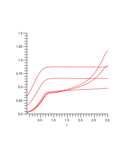
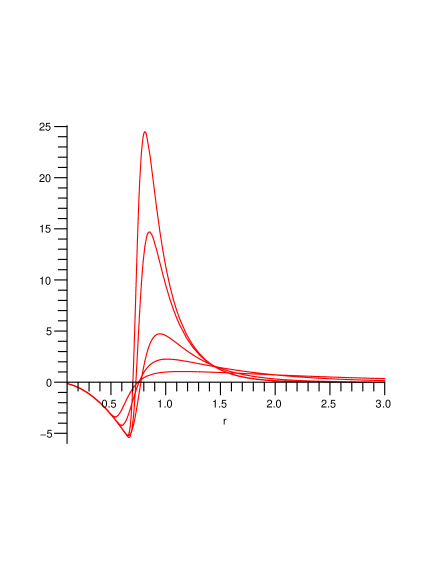
FIG. 1.: (Color online) (a) The function $f(r)$ for $\Gamma=0.1,0.3,1,2,2.2$ (top to bottom at the l.h.s.). (b) The integrand $4\pi\,r^{2}\,\delta n(r)$ for the same values of the coupling. Larger couplings produce higher peaks.

We set $n=1$ below and seek a radial solution of the form

$$\phi(r)=f(r)\,\frac{e^{-\kappa r}}{r}$$ (56)

with $\kappa=\sqrt{4\pi\Gamma}$ the Debye-H$\ddot{\rm{u}}$ckel inverse radius. One may think of $f(r)$ as of an effective coupling. The value $f(r)=1$ corresponds to the normalized solution of the linearized theory. If one includes the repulsive core at small distances, in weak coupling f(r) remains an r-independent constant, although different from 1. As we will see, at stronger coupling the deviations of f(r) from a constant value will display deviations from the linear Debye-H$\ddot{\rm{u}}$ckel theory.

Inserting (56) into (53) allows for numerical solutions for weak and strong coupling. At large distances, the screened potential is weak and the linear Debye-H$\ddot{\rm{u}}$ckel theory is valid with $f(r)$ asymptotic a constant. The latter is fixed by the normalization (55). The numerical results for $f(r)$ for different $\Gamma$ are shown in Fig. 1(a). As expected, for $\Gamma<1$ the function $f(r)$ asymptotes a constant, except at small distances where the linearized theory never works. For $\Gamma>2$ one enters a domain where $f(r)$ is changing dramatically. We found that for $\Gamma>2$ the modification is fast growing, indicating a beginning of a phenomenon known as “over-screening”. At large $\Gamma$ our solution is large and oscillating, which indicate not only large deviations from a Debye theory but actually a complete breaking of the mean field approach itself. Such erratic solutions are a precursor for highly correlated state, beyond spherical mean field, and eventually a complete crystallization at very large $\Gamma$ .

The generalization of these results to a non-Abelian colored plasma is straightforward. In the $SU(2)$ case, the original point charge can be thought of as having a particular color direction, while those in a screening cloud have any charges. As a result, there is an angular variable $z={\rm cos}(\theta)=\hat{Q}\cdot\hat{Q}_{0}$ in the Boltzmann factor as in (20). The potential $\Phi_{SU2}$ averaged over the color orientations is

$$\Phi_{SU2}=\frac{1}{2}\int_{-1}^{1}dz\,z\,e^{zA}=\frac{{\rm ch}A}{2A}-\frac{{\rm sh}A}{2A^{2}}$$ (57)

where $A=\Gamma\Phi$ is the Coulomb part. The Casimir is absorbed in $\Gamma$. These factors are reminiscent of the $e^{\pm 3\epsilon}$ in the virial expansion and have the same origin. (57) is plotted in Fig 2 along with its asymptote. The linear non-Abelian mean-field solution follows from the Abelian one by multiplying the squared Debye mass by $<z^{2}>=1/3$. Other gauge groups can be treated in the the same way. Indeed, in the $SU(3)$ case the averaging over angles include 6 variables (the 8 generators minus the 2 Casimirs) in the pertinent invariant measure.

FIG. 2.: (Color online) $\Phi_{SU2}(r)$ (upper curve) with its small $A/3$ and large $e^{A}\,(A-1)/2A^{2}$ expansion.

V Nonlinear Screening through a Coulomb Crystal

As we pointed out before, at very large $\Gamma$ or very small $T$ the system freezes into a crystal. To understand the difference between screening in the Debye-H$\ddot{\rm{u}}$ckel limit and the screening in the crystalline phase, we discuss the induced potentials and the behavior of their pertinent partition functions.

In the Debye limit the induced potential at small and intermediate coupling is of the form

$$V_{D}(r)=-{Q\over r}\left(1-e^{-{r/R_{D}}}\right)\approx-{Q\over R_{D}}\left(1-{r/2R_{D}}+...\right)$$ (58)

The induced potential is finite at small $r$ and rises linearly with $r$. The pertinent classical partition function in the Einstein approximation (ignoring coupling between oscillations of different charges) is

$$Z\approx\int d^{3}r\,e^{-{V_{D}/T}}\approx T^{3}\,e^{Q/T\,R_{D}}$$ (59)

In a crystal the induced potential by all charges except one is quite different. If one starts with a pure Coulomb field in a cubic crystal, then

$$V(\vec{r})=\sum_{n_{i}=-n_{max}}^{n_{max}}{(-1)^{\sum n_{i}}\over|\vec{r}-\vec{n}|}-{1\over|\vec{r}|}$$ (60)

where we introduced a cutoff of the sum $n_{max}$ and also subtracted the $n_{x}=n_{y}=n_{z}=0$ term. The alternating signs cause the sum to converge. To smoothen-out the oscillations between even-odd finite $n_{max}$ we use instead

$$\bar{V}(x,y,z)={V(n_{max})+V(n_{max}+1)\over 2}$$ (61)

which is within few percent of the limit already at $nmax=3$. The convergence is related to the fact that new distant charges added between $n_{max}$ and $n_{max}+1$ do not have a nonzero dipole or quadrupole contribution. In fact they start contributing to the l=4 octupole. As a result, the field is extremely flat at small $r$ (near the origin) with only quartic $r^{4}$ corrections to the constant $V(0)$, see Fig.3. This is just Madelung constant which is the energy of the ideal zero $T$ crystal (in our case it is 1.75). The figure shows also high multiples in the angular distribution, with alternating positive and negative (unstable) directions.

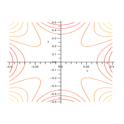
FIG. 3.: (Color online) Contour plot of the Coulomb potential in the z=0 plane versus x and y (in units of the nearest neighbor distance) as induced by all charges except one in a cubic crystal.

We note that the potential used in our molecular simulations in [7] has in addition a repulsive core needed to prevent collapse at short distances. The result is a quadratic instead of quartic potential at the origin as is seen in Fig. 4, with $V(r)\approx 9r^{2}$ near the origin. The pertinent partition function in the Einstein approximation is then

$$Z\approx\int d^{3}r\,e^{-{V/T}}=\left({\pi T\over 9}\right)^{3/2}\,,$$ (62)

which leads to the usual classical potential energy of oscillations $3T/2$. However, as we have shown above, in order to understand the MD data one has to include the oscillations of the color vectors as well.

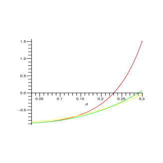
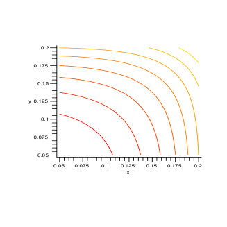
FIG. 4.: (Color online) Induced potential with Coulomb and repulsive core in the z=0 plane: (a) along the crystal axes (green) and the diagonal (red), along with the fit (yellow). (b) Planar contour plot for a cubic crystal.

VI From Debye-H$\ddot{\rm{u}}$ckel Screening to Debye Crystal

As the density is increased or equivalently the coupling is increased or the temperature is decreased, the potential effects dominate over the kinetic effects in the cQGP. $\Gamma$ which is the ratio of the potential to kinetic energy is then large. For simplicity and to compare with the molecular dynamics results in I, we specialize in this section to one species, say gluons only. Let $\Gamma$ be the standard cQGP plasma parameter defined as [7]

$$\Gamma=\frac{\rm potential}{\rm kinetic}=\frac{C_{2}\alpha_{s}/a_{WS}}{T}\,,$$ (63)

with the Wigner-Seitz radius satisfying $c\,(4\pi\,a^{3}_{WS}/3)=1$. In terms of (63) the excess free energy $\bf{F}_{\rm ex}$ is

$${\bf F}(\Gamma)={\bf F}(0)+\bf{F}_{\rm ex}(\Gamma)$$ (64)

and measures the Coulomb interacting part of the free energy. In the cQGP the excess free energy $\bf{F}_{\rm ex}$ per particle is the Debye-H$\ddot{\rm{u}}$ckel contribution

$$\frac{\bf{F}_{\rm DH}}{N\,T}= (N_{c}^{2}-1)\,\frac{1}{2}\int\frac{d^{3}q}{(2\pi)^{3}}\left({\rm ln}\left(1+\frac{K^{2}}{q^{2}}\right)-\frac{K^{2}}{q^{2}}\right)$$ (65)

$$= -(N_{c}^{2}-1)\frac{\Gamma^{3/2}}{\sqrt{3}}\,,$$ (66)

which is finite, attractive and nonlinear in the concentration $c$.

The higher order corrections in the concentration and/or coupling were discussed above and will not be repeated. Instead, here we note that (66) is finite and involves an integration over small as well as large momenta. As the density is increased in the cQGP there is increasing local ordering due to the strong colored Coulomb attractions causing the dilute and screened gas to undergo changes to a liquid and eventually to a crystal.

Following Debye description of solids, we will assume that the allowed momenta in (66) are those commensurate with the total number of degrees of freedom,

$$2\int_{0}^{q_{D}}\frac{V\,d^{3}q}{(2\pi)^{3}}=3\,N\,d$$ (67)

which fixes the Debye cutoff $q_{D}=\pi\,(9d\,c)^{1/3}$. For every particle moving in 3d space there are attached $d=N_{c}(N_{c}-1)/2$ independent but classical color charges. The cutoff Debye-H$\ddot{\rm{u}}$ckel contribution is

$$\frac{\bf{F}_{\rm DH}}{N\,T}=(N_{c}^{2}-1)\,\frac{q_{D}^{3}}{8\pi^{2}}$$ (68)

$$\times\,\int_{0}^{1}\,x^{2}\,dx\,\left({\rm ln}\left(1+\frac{A\,\Gamma}{x^{2}}\right)-\frac{A\,\Gamma}{x^{2}}\right)$$ (69)

The integrals are readily undone and the answer is

$$\frac{\bf{F}_{\rm DH}}{N\,T}=-(N_{c}^{2}-1)\,\frac{3d}{2}$$ (70)

$$\times\,\left((A\Gamma)^{3/2}\,{\rm atan}(1/\sqrt{A\Gamma})-\frac{1}{2}({\rm ln}(1+A\Gamma)-A\Gamma)\right)$$ (71)

with $A=(2/3)(2/(\pi\,d)^{2})^{1/3}$. A similar construction was suggested by Brilliantov for the Abelian one component plasma [14]. The excess energy following from (71) is ${{\bf U}}_{\rm ex}=\partial\bf{F}_{\rm DH}/\partial{\rm ln}\Gamma$ which is

$$\frac{{\bf U}_{\rm ex}}{N\,T}=-(N_{c}^{2}-1)\,\frac{9d}{4}\left((A\Gamma)^{3/2}\,{\rm atan}(1/\sqrt{A\Gamma})\right)$$ (72)

For small $\Gamma$ we recover the (linear) Debye-H$\ddot{\rm{u}}$ckel limit, while for large $\Gamma$ we obtain

$$\frac{{\bf U}_{\rm ex}}{N\,T} = -(N_{c}^{2}-1)\,\frac{9d}{4}\left(A\,\Gamma-{1\over 3}\right)+{\cal O}(\Gamma^{-1})$$ (73)

$$= -c_{MD}\,\Gamma+{9\over 4}$$ (74)

where the Madelung constant is $c_{MD}$. For $N_{c}=2$: $d=1$, $A\approx 0.392$ and $c_{MD}=2.64$

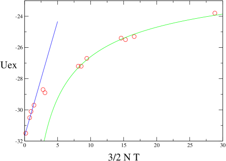
FIG. 5.: (Color online) Potential energy as a function of kinetic energy, $(3/2)NT$ for N=64 particles is N=64. The red points are the MD simulations, their statistical accuracy (not shown) is estimated to be 7 percents for all points. The blue line is a fit to eq. (75). the green curve is a fit to eq. (78).

This excess potential energy was calculated numerically in I for the one-species cQGP with $N_{c}=2$ using molecular dynamics. Figure 5 shows the plot of the excess potential energy as a function of the total kinetic energy, $(3/2)NT$. The region of small temperature corresponds to large $\Gamma$ while the region with large temperature to small $\Gamma$. For points corresponding to $\Gamma\approx 16-131$ the excess energy can be approximated by 

$${{\bf U}_{ex}\over N}\approx-0.5+2.25\,T\,.$$ (75)

The numerical crystal analysis of section V yields the following excess energy per particle

$${{\bf U}_{ex}\over N}\approx-0.44+2.5\,T\,$$ (76)

with $3T/2$ following from the oscillation energy in the harmonic potential, plus $1\,T$ from the oscillations of the classical $SU(2)$ color degrees of freedom . One can see that at least the specific heat of a low-T colored crystal is well reproduced.

Using the definition of $\Gamma$ in (63) in (74) the excess energy per particle following from the Debye interpolation as a function of temperature is

$${{\bf U}_{ex}\over N}\approx-0.65+2.25\,T.$$ (77)

which is in in good agreement with the molecular dynamics result at small temperature or large $\Gamma$. In the dimensionless units of the Appendix, the conversion from $T$ to $\Gamma$ is given by $\Gamma=0.25/T$.

In the intermediate coupling regime with $\Gamma\approx 0.8-3$, we enter the liquid regime of the cQGP (the right part of the figure as small $\Gamma$ means high $T$). Numerically,

$${{\bf U}_{ex}\over N}\approx-0.3-{0.03\over\sqrt{T}}$$ (78)

The Debye-Huckel limit predicts ${\bf U}_{ex}/N=-0.3/\sqrt{T}$ at large $T$ or weak coupling but not the large negative constant. Its appearance can be traced back to the appearance of a sharp peak in the inter-particle distance at about $1/n^{1/3}$ as shown in Fig.1b in the liquid phase. In the gas phase, the the peak is spread in the form of a large Debye cloud. The negative constant contribution to the energy in (78) corresponds to the potential following from this peak.

VII Summary

We have analyzed the screening and thermodynamics of a strongly coupled classical colored QGP. The basic question we asked in this paper was when and whether one can relate the textbook theories, such as Debye-H$\ddot{\rm{u}}$ckel screening or virial expansion, to our MD data.

We have identified the onset of nonlinear screening using the mean field approach, as well as onset of the correlations using a low density expansion around the mean field. We have carried explicitly the expression for the pressure of the cQGP to order $c^{5/2}$. Not unexpectedly, we have found that the textbook methods are not really applicable in the liquid regime we studied. In particular, the spherically symmetric mean field treatment is very unstable already at medium coupling, and the virial expansion fails at very small densities. Both are signals for the onset of a cluster formation (liquid) or long range ordering (crystal).

We hope to address more issues in forthcoming publications. In particular, issues related to the collective excitations of the system (sound and plasma-color waves), and propagation of external bodies in QGP (jet energy loss) etc.

Appendix

In this appendix we briefly discuss the units that were used in I: length, time and mass. The unit of length was chosen as the separation between two particles, $r=\tilde{\lambda}$, at which the potential (the sum of Coulomb and core) is minimum. The density or concentration of particles $n=c$, is dimensionless in these units. All simulations in I were carried with $n=c=0.3676$. The unit of time $\tau_{0}$ was set by the plasma frequency

$$\tau_{0}=\omega_{p}^{-1}=({m\over 4\pi ne^{2}})^{1/2}\,,$$ (79)

with $e^{2}=C_{2}\alpha_{s}$ in the non-Abelian case. The unit of mass was set by the particles energy $m$.

All dimensional quantities can be expressed using these basic units. For instance, the kinetic energy is measured in units of $m{\tilde{\lambda}}^{2}/\tau_{0}^{2}$. All simulations in I were carried with $n=c=0.3676$ and $\tilde{\lambda}=1$, $m=1$ and $\tau_{0}=1$. With these conventions, the comparison with the molecular dynamics uses $a_{WS}=0.866$, $C_{2}\alpha_{s}=0.216$ and $\Gamma=0.25/T$.

Acknowledgments.  

This work was partially supported by the US-DOE grants DE-FG02-88ER40388 and DE-FG03-97ER4014.

REFERENCES

- [1] E. V. Shuryak, Phys. Lett. B78 (1978) 150; Yadernaya Fizika 28 (1978) 796; Phys.Rep. 61 (1980) 71.
- [2] E. Braaten and R. D. Pisarski, Nucl. Phys. B 337 (1990) 569.
- [3] D. Teaney, J. Lauret and E. V. Shuryak, Phys. Rev. Lett. 86 (2001) 4783; P.F. Kolb, P.Huovinen, U. Heinz, H. Heiselberg, Phys. Lett. B500 (2001) 232; Review in P. F. Kolb and U. Heinz, nucl-th/0305084.
- [4] E. Shuryak, Prog. Part. Nucl. Phys. 53 (2004) 273.
- [5] E. V. Shuryak and I. Zahed, Phys. Rev. C 70 (2004) 021901; Phys. Rev. D 70 (2004) 054507.
- [6] M. Asakawa and T. Hatsuda, Nucl. Phys. A715 863c (2003); S. Datta, F. Karsch, P. Petreczky and I. Wetzorke, Nucl. Phys. Proc. Suppl. 119 (2003) 487.
- [7] B.A. Gelman, E.V. Shuryak and I. Zahed, nucl-th/0601029.
- [8] J.M. Caillol, cond-mat/0305465 and references therein.
- [9] K. Johnson, Ann. Phys. (N.Y.) 192 (1989) 104.
- [10] S.K. Wong, Nuovo Cimento A 65 (1970) 689.
- [11] O. Kaczmarek, S. Ejiri, F. Karsch, E. Laermann and F. Zantow, hep-lat/0312015.
- [12] S.Ichimaru, H.Iyetomi and S.Tanaka, Phys.Rep.149 (1986) 92-205
- [13] J.P.Hansen and I.R.McDonald, Phys.Rev.A11 (1975) 2111.
- [14] N. Brilliantov, cond-mat/9805358
- [15] A.Yu.Grosberg, T.T.Nguyen and B.I.Shklovkii, cond.-mat/0105140.