Universal scaling of the elliptic flow at RHIC

Abstract

Recent PHOBOS measurements of the excitation function for the pseudo-rapidity dependence of elliptic flow in Au+Au collisions at RHIC, have posed a significant theoretical challenge. We show here that these data are described by the Buda-Lund model. A universal scaling curve, predicted by the Buda-Lund hydro model, describes not only PHOBOS data, but also recent, detailed PHENIX and STAR elliptic flow data. This is a consequence of perfect fluid hydrodynamics as implemented in the Buda-Lund hydro model.

Introduction, terminology. One of the unexpected results from experiments at the Relativistic Heavy Ion Collider (RHIC) is the relatively strong second harmonic moment of the transverse momentum distribution, referred to as the elliptic flow. Measurements of the elliptic flow by the PHENIX, PHOBOS and STAR collaborations (see refs. [1, 2, 3, 4, 5]) reveal rich details in terms of its dependence on particle type, transverse ($p_{T}$) and longitudinal momentum ($\eta$) variables, and on the centrality and the bombarding energy of the collision. In the soft transverse momentum region ($p_{T}\lesssim 2$ GeV/c), the measurements at mid-rapidity are found to be reasonably well described by hydrodynamical models [6, 7]. By contrast, differential measurement of the pseudo-rapidity dependence of elliptic flow $v_{2}(\eta)$, and its excitation function have resisted several attempts at a description in terms of hydrodynamical models (but see their new description by the SPHERIO model [8]). Here we show that these data are consistent with the theoretical and analytic predictions that are based on Eqs. (1-6) of Ref. [9], that is, on perfect fluid hydrodynamics.

There is a confusion in the literature if perfect or perhaps an ideal fluid has been produced in Au+Au collisions at RHIC. The BNL press release [10] uses the terminology “perfect liquid”. On the other hand, some other authors, for example refs. [11, 12] are using a different terminology: “ideal fluid”.

Although in many cases these different terms refer to the same set of equations, let us clarify that in fact there is a distinction between ideal and perfect liquids and the corresponding hydrodynamical equations. The expression “ideal fluid” is frequently used either 1: for an inviscid, incompressible fluid, or 2: for an inviscid fluid. These definitions of “ideal fluid” are inequivalent, and one should note that definition 1 that includes the incompressibility is more frequent, as it is part of the primary physics courses: “an ideal fluid keeps its volume but conforms to the outline of its container”.

Let us also consider the definitions of perfect liquids. A perfect liquid is defined also in two different ways: 1: A fluid which looks isotropic in its rest frame is called a perfect fluid. 2: A fluid which has no shear stresses, viscosity or heat conduction is a perfect fluid. It turns out that these two definitions of the perfect fluids are equivalent. Perfect fluids are frequently used in general relativity to model idealized distributions of matter. This terminology, with clear definition of the energy-momentum tensor that is diagonal in the rest frame of the matter, has also been adopted by the Particle Data Group [13]. When considering these questions on terminology, it is important to note that lack of viscosity does not yet imply that a fluid is perfect, as the lack of heat conduction and the vanishing of shear tensor needs also be discussed. Second, it is clear that we are discussing the time evolution of an exploding fireball, so an ideal fluid of a time independent volume is irrelevant for this problem, in contrast to def. 1 of ideal fluids.

In conclusion, we will continue to use the well defined and unambigous terminology of “perfect fluid” hydrodynamics in context of RHIC physics, and strongly recommend it also for other authors to avoid confusion on this subject.

The Buda-Lund hydro model. The tool used to describe the pseudorapidity-dependent elliptic flow is the Buda-Lund hydro model. This hydro model [14, 15] is based on exact analytic hydro solutions discussed in Refs. [16, 17]. Buda-Lund type of exact, parametric hydro solutions are being explored at the moment as well. General, non-relativistic, ellipsoidally expanding solutions [16], and relativistic but non-accelerating solutions [17, 18] are known. An important missing link is the family of finite, relativistic, accelerating solutions which currently being pursued [19].

The Buda-Lund hydro model is successful in describing the BRAHMS, PHENIX, PHOBOS and STAR data on identified single particle spectra and the transverse mass dependent Bose-Einstein or HBT radii as well as the pseudorapidity distribution of charged particles in Au + Au collisions both at $\sqrt{s_{\rm{NN}}}=130\,$GeV [20] and at $\sqrt{s_{\rm{NN}}}=200\,$GeV [21]. The model is defined with the help of its emission function; to take into account the effects of long-lived resonances, it utilizes the core-halo model [22], and characterizes the system with a hydrodynamically evolving core and a halo of the decay products of the long-lived resonances.

The elliptic flow would be zero in an axially symmetric case, so we developed an ellipsoidal generalization of the model that describes an expanding ellipsoid with principal axes $X$, $Y$ and $Z$. Their derivatives with respect to proper-time (expansion rates) are denoted by $\dot{X}$, $\dot{Y}$ and $\dot{Z}$. The generalization goes back to the original one, if the transverse directed principal axes of the ellipsoid are equal, ie $X=Y$ (and also $\dot{X}=\dot{Y}$). The deviation from axial symmetry can be measured by the momentum-space eccentricity,

$$\epsilon_{p}=\frac{\dot{X}^{2}-\dot{Y}^{2}}{\dot{X}^{2}+\dot{Y}^{2}}.$$ (1)

The exact analytic solutions of hydrodynamics [9, 23, 24], which form the basis of the Buda-Lund hydro model, develop Hubble-flow for late times, ie $X\rightarrow_{\tau\rightarrow\infty}\dot{X}\tau$, so the momentum-space eccentricity $\epsilon_{p}$ nearly equals space-time eccentricity $\epsilon$. It turns out that the data fitting is easier if instead of $\dot{X}$ and $\dot{Y}$ the eccentricity variable $\epsilon$ is introduced and complemented by the average radial flow defined as $\langle u_{t}\rangle=1/2/\sqrt{1/\dot{X}^{2}+1/\dot{Y}^{2}}$. Obviously, the expansion rates are given as and $\dot{X}=\langle u_{t}\rangle/\sqrt{1-\epsilon_{p}}$ and $\dot{Y}=\langle u_{t}\rangle/\sqrt{1+\epsilon_{p}}$.

Let us introduce $\Delta\,\eta$ additionally. It represents the elongation of the source expressed in units of space-time rapidity. Let us consider furthermore that at the freeze-out $\tau\,\Delta\eta=Z$ and $Z\approx\dot{Z}\,\tau$, and so $\Delta\eta\approx\dot{Z}$. Hence, in this paper we extract space-time eccentricity ($\epsilon$), average transverse flow ($u_{t}$) and longitudinal elongation ($\Delta\eta$) from the data, instead of $\dot{X}$, $\dot{Y}$ and $\dot{Z}$.

Although the proof of Ref. [25] was given only for the case of exact parametric solutions of non-relativistic hydrodynamics, we expect a similar behavior at the end of relativistic expansions just as well, because the acceleration of the scales $(X,Y,Z)$ is due to pressure gradients. However, the pressure hence its gradients as well tend to vanishing values in the late stages of both the non-relativistic [23, 24, 25] and relativistic [9, 17] exact parametric solutions of hydrodynamics.

In the time dependent hydrodynamical solutions, these values evolve in time, however, it was show in Ref. [25] that $\dot{X}$, $\dot{Y}$ and $\dot{Z}$, and so $\epsilon$, $u_{t}$ and $\Delta\eta$ become constants of the motion in the late stages of the expansion.

Elliptic flow from the model. The result for the elliptic flow is the following simple universal scaling law:

$$v_{2}=\frac{I_{1}(w)}{I_{0}(w)},$$ (2)

where $I_{n}$ is the modified Bessel function of order $n$. For other flow coefficients, the prediction is also simple and universal:

$$v_{2n} = I_{n}(w)/I_{0}(w),$$ (3)

$$v_{2n+1} = 0.$$ (4)

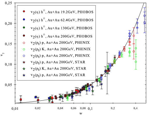
The model thus predicts a scaling law, valid under certain conditions detailed in Ref. [15], fulfilled by these data : every $v_{2}$ measurement falls on the same universal curve of $I_{1}/I_{0}$ when plotted against $w$.

This means, that $v_{2}$ depends on any measurable quantity only through the scaling parameter $w$. In practice this implies that the detailed and experimentally known dependence of the elliptic flow on transverse or longitudinal momentum, center of mass energy, centrality, type of the colliding nucleus etc is only apparent.

Before giving the definition of the scaling variable $w$ it is educational to introduce the effective temperatures or slope parameters in the impact parameter direction ($T_{x}$) and in the direction out of the reaction plane ($T_{y}$), as follows:

$$T_{x} = T_{0}+\overline{m}_{t}\,\dot{X}^{2}\frac{T_{0}}{T_{0}+\overline{m}_{t}a^{2}},$$ (5)

$$T_{y} = T_{0}+\overline{m}_{t}\,\dot{Y}^{2}\frac{T_{0}}{T_{0}+\overline{m}_{t}a^{2}},$$ (6)

and

$$\overline{m}_{t}=m_{t}\cosh(\eta_{s}-y).$$ (7)

Here $m_{t}=\sqrt{m^{2}+p_{x}^{2}+p_{y}^{2}}$ is the transverse mass, $a=\langle\Delta T/T\rangle_{t}=(T_{0}-T_{s})/T_{s}$ measures the temperature gradient in the transverse direction, at the mean freeze-out time, where $T_{0}$ the central temperature at the mean freeze-out time while $T_{s}$ is the temperature of the surface of the fireball. Also we introduce a lengthscale, $R_{s}$, defined by the transverse coordinate where the temperature distribution decreases to half, as compared to the center, so $T(r_{x}=r_{y}=R_{s})=T_{0}/2$. In this notation, a flat temperature profile corresponds to the $R_{s}\rightarrow\infty$ limit.

Furhermore, $\eta_{s}$ is the space-time rapidity of the saddle-point (point of maximal emittivity), which depends on the rapidity, the longitudinal expansion, the transverse mass and on the central freeze-out temperature $\eta_{s}-y=\frac{y}{1+\Delta\eta\frac{m_{t}}{T_{0}}},$ where $y=0.5\log(\frac{E+p_{z}}{E-p_{z}})$ is the rapidity. Because of this, at midrapidity, where PHENIX and STAR $v_{2}(p_{t})$ data was taken, Eq. (7) simplifies to $\overline{m}_{t}=m_{t}$. These definitions imply that the effective temperature is transverse mass and rapidity dependent both in the reaction plane and out of the reaction plane direction,

The effective slope parameter, $T_{*}$, of the asimuthally averaged single particle spectra can be defined as

$$\frac{1}{T_{*}}=\frac{1}{2}\left(\frac{1}{T_{x}}+\frac{1}{T_{y}}\right).$$ (8)

A relativistic generalization of the kinetic energy, relevant for the elliptic flow analysis is defined as

$$E_{K}=\frac{p_{t}^{2}}{2\overline{m}_{t}}$$ (9)

Finally, the eccentricity of the single particle spectra can be defined as

$$\varepsilon=\frac{T_{x}-T_{y}}{T_{x}+T_{y}}.$$ (10)

The universal scaling variable $w$ turns out to be the product

$$w=\frac{E_{K}}{2T_{*}}\varepsilon$$ (11)

It is interesting to note, that each of the kinetic energy term, the effective temperature $T_{*}$ and the momentum space eccentricity $\varepsilon$ are transverse mass and rapidity dependent factors. However, for $\overline{m}_{t}/T_{0}\gg 1$, $\varepsilon\rightarrow\varepsilon_{p}=\frac{\dot{X}^{2}-\dot{Y}^{2}}{\dot{X}^{2}+\dot{Y}^{2}}$ becomes independent of transverse mass and rapidity.

This structure of the universal scaling variable suggests that the detailed centrality, transverse mass and rapidity dependence of the elliptic flow is only apparent, and the Buda-Lund model predicts that when plotted against the scaling variable $w$, a data collapsing behavior sets in and a universal scaling curve emerges, which coincides with the ratio of the above two Bessel functions. Additional details about the ellipsoidally symmetric model and its result on $v_{2}(\eta)$ can be found in Ref. [15].

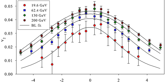
Eq. (2) depends, for a given centrality class, on rapidity $y$ and transverse mass $m_{t}$. Before comparing our result to the $v_{2}(\eta)$ data of PHOBOS, we thus performed a saddle point integration in the transverse momentum variable and performed a change of variables to the pseudo-rapidity $\eta=0.5\log(\frac{|p|+p_{z}}{|p|-p_{z}})$, similarly to Ref. [26]. This way, we have evaluated the single-particle invariant spectra in terms of the variables $\eta$ and $\phi$, and calculated $v_{2}(\eta)$ from this distribution, a procedure corresponding to the PHOBOS measurement described in Ref. [1].

Transverse momentum dependent elliptic flow data at mid-rapidity can also be compared to the Buda-Lund result directly, as it was done in e.g. Ref. [15].

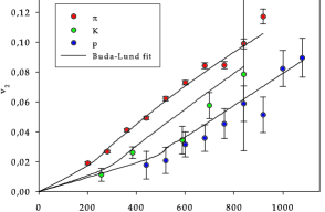
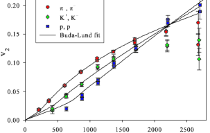
Comparison to experimental data. When fitting only $v_{2}(p_{t})$ data of identified particles as measured by STAR and PHENIX, we have found that fit parameters $u_{t}$ and $\epsilon$ are essential. When analysing $v_{2}(\eta)$ data, we found that they can be described by a two-parameter fit: parameter $\epsilon$ controls the peak while parameter $\Delta\eta$ controlls the widht of these distributions. Note that the same $\Delta\eta$ parameter controlls the width of the pseudo-rapidity distribution as well, but these simultaneous fits will be reported elsewhere. The quality of our fits was found to be insensitive to the precise value of other parameters of the model. Hence we have fixed their values. We also excluded points with large rapidity from lower center of mass energies $v_{2}(\eta)$ fits ($\eta>4$ for 19.6 GeV, $\eta>4.5$ for 62.4 GeV) and points with large transverse momentum ($p_{t}>1.3$ GeV) from $v_{2}(p_{t})$ fits.

Fits to PHOBOS data of Ref. [1], PHENIX data of Ref. [2] and STAR data of Ref. [3] are shown in the top three panels of Fig. 1. Bottom panel of Fig. 1 demonstrates that the investigated PHOBOS, PHENIX and STAR data points follow the theoretically predicted scaling law. The fitting package is available at Ref. [27], and the fits can be redone on the interactive online Buda-Lund page [28].

In contrast, Ref. [12] considered the description of the centrality and pseudorapidity dependence of the elliptic flow in 200 GeV Au+Au collisions as measured by the PHOBOS collaboration in Ref. [1], however, this attempt failed to describe these data in a unified framework and concluded, that “whether all of the observed discrepancies between elliptic flow data and … simulations can be blamed on ’late hadronic viscosity’ … depends on presently unknown details of the initial state of the matter formed in heavy-ion collisions”.

This failure can be contrasted to the success of the Buda-Lund hydro model, that analytically predicted the scaling properties of elliptic flow in 2003. The particle mass, transverse momentum, pseudorapidity and centrality dependence of the elliptic flow at RHIC are being fully explored only now in experimental studies. We think that one of the important elements of success was that the Buda-Lund hydro model was based on exact, parametric and analytic solutions of hydrodynamics. These solutions were found recently for both non-relativistic and relativistic kinematic domain. Non-relativistic solutions include refs. [23, 24, 25]. Relativistic solutions include not only the Hwa-Bjorken and the Hubble solutions but their new relativistic generalizations for 1+1 dimensional, 1+3 dimensional axially symmetric, and ellipsoidally symmetric solutions, see refs. [9, 17].

Conclusions. In summary, we have shown that the excitation function of the transverse momentum and pseudorapidity dependence of the elliptic flow in Au+Au collisions is well described by the Buda-Lund model. We have thus provided a quantitative evidence of the validity of the perfect fluid picture of soft particle production in Au+Au collisions at RHIC. This perfect fluid extends far away from mid-rapidity. The universal scaling of PHOBOS $v_{2}(\eta)$ and PHENIX and STAR $v_{2}(p_{t})$, expressed by Eq. (2) and illustrated by Fig. 1 provides a successful quantitative as well as qualitative test for the appearance of a perfect fluid in Au+Au collisions at various colliding energies at RHIC.

Acknowledgments. T. Cs. is greatful for B. L. for a kind hospitality at the University of Lund. This research was supported by the NATO Collaborative Linkage Grant PST.CLG.980086, by the Hungarian - US MTA OTKA NSF grant INT0089462, by the OTKA grants T038406, T049466, by a KBN-OM Hungarian - Polish programme in S&T.

	PHOBOS Au+Au $v_{2}(\eta)$
	19.6 GeV		62.4 GeV		130 GeV		200 GeV
$\epsilon$	0.30	$\pm$0.03	0.37	$\pm$0.01	0.40	$\pm$0.01	0.42	$\pm$0.01
$\Delta\eta$	2.0	$\pm$0.3	2.28	$\pm$0.05	2.60	$\pm$0.04	2.70	$\pm$0.04
$\chi^{2}$/NDF	1.9/11		21/13		36/15		26/15
conf. level	100%		19%		0.78%		6.2%

	PHENIX 200GeV Au+Au $v_{2}(p_{t})$						STAR
	$\pi$		K		p		$\pi$, K, p
$\epsilon$	0.31	$\pm$0.003	0.32	$\pm$0.04	0.3	$\pm$0.1	0.38	$\pm$0.01
$u_{t}$	1.2	$\pm$0.1	0.7	$\pm$0.12	0.6	$\pm$0.3	1.0	$\pm$0.1
$\chi^{2}$/NDF	21/7		5/5		10/2		45/21
conf. level	2%		80%		8%		0.5%

Table 1.: Results of fits to data of PHOBOS [1], PHENIX [2] and STAR [3]. Fixed parameters: $T_{0}=200$ MeV, $a=$1, and for $v_{2}(\eta)$, $u_{t}=1.5$. Note that data from PHOBOS, PHENIX and STAR have different centrality selection.

Fig. 1.: STAR [3] (top left), PHENIX [2] (top right) and PHOBOS [1] (middle) data on elliptic flow, $v_{2}$, plotted versus $p_{t}$ and $\eta$ and fitted with Buda-Lund model. Bottom: elliptic flow versus variable $w$ is plotted. The data points show the predicted [15] universal scaling.

References

- [1] B. B. Back et al., Phys. Rev. Lett. 94, 122303 (2005)
- [2] S. S. Adler et al., Phys. Rev. Lett. 91, 182301 (2003)
- [3] J. Adams et al. [STAR Collaboration], arXiv:nucl-ex/0409033.
- [4] C. Adler et al., Phys. Rev. Lett. 87, 182301 (2001)
- [5] P. Sorensen et al., J. Phys. G 30, S217 (2004)
- [6] K. Adcox et al., Nucl. Phys. A 757, 184 (2005)
- [7] J. Adams et al., Nucl. Phys. A 757, 102 (2005)
- [8] F. Grassi, Y. Hama, O. Socolowski and T. Kodama, J. Phys. G 31, S1041 (2005).
- [9] T. Csörgő, L. P. Csernai, Y. Hama and T. Kodama, Heavy Ion Phys. A 21, 73 (2004)
- [10] http://www.bnl.gov/bnlweb/pubaf/pr/PR_display.asp?prID=05-38
- [11] A. Peshier and W. Cassing, Phys. Rev. Lett. 94, 172301 (2005)
- [12] T. Hirano, U. W. Heinz, D. Kharzeev, R. Lacey and Y. Nara, nucl-th/0511046.
- [13] http://pdg.lbl.gov/2005/reviews/bigbangrpp.pdf
- [14] T. Csörgő and B. Lörstad, Phys. Rev. C 54 (1996) 1390
- [15] M. Csanád, T. Csörgő and B. Lörstad, Nucl. Phys. A 742, 80 (2004)
- [16] T. Csörgő, S. V. Akkelin, Y. Hama, B. Lukács and Y. M. Sinyukov, Phys. Rev. C 67, 034904 (2003)
- [17] T. Csörgő, F. Grassi, Y. Hama and T. Kodama, Phys. Lett. B 565, 107 (2003)
- [18] Y. M. Sinyukov and I. A. Karpenko, arXiv:nucl-th/0506002.
- [19] M. Nagy, T. Csörgő, M. Csanád, In preparation
- [20] M. Csanád, T. Csörgő, B. Lörstad, A. Ster, Act. Phys. Pol. B35, 191 (2004)
- [21] M. Csanád, T. Csörgő, B. Lörstad and A. Ster, Nukleonika 49, S45 (2004)
- [22] T. Csörgő, B. Lörstad and J. Zimányi, Z. Phys. C 71, 491 (1996)
- [23] S. V. Akkelin, T. Csörgő, B. Lukács, Y. M. Sinyukov, M. Weiner, Phys. Lett. B 505, 64 (2001)
- [24] T. Csörgő, Acta Phys. Polon. B 37, 483-494 (2006)
- [25] T. Csörgő and J. Zimányi, Heavy Ion Phys. 17, 281 (2003)
- [26] D. Kharzeev and E. Levin, Phys. Lett. B 523, 79 (2001)
-
[27]
PHENIX CVS: offline/analysis/budalund/ -
[28]
http://csanad.web.elte.hu/budalund/ - [29] R. A. Lacey, nucl-ex/0510029.
- [30] M. Csanád, T. Csörgő, B. Lörstad and A. Ster, nucl-th/0510027.
- [31] M. Csanád, T. Csörgő, B. Lörstad and A. Ster, nucl-th/0509106.