APPLICATIONS OF CONTINUUM SHELL MODEL

Abstract

The nuclear many-body problem at the limits of stability is considered in the framework of the Continuum Shell Model that allows a unified description of intrinsic structure and reactions. Technical details behind the method are highlighted and practical applications combining the reaction and structure pictures are presented.

1 Introduction

In this presentation we discuss specific features of the Continuum Shell Model (CoSMo), the approach based on the projection formalism [1], formulated in the classical book [2] and developed into a practical instrument in Refs. [3, 4]. The whole problem of many-body physics on the verge of stability has been extensively explored in the past, especially in relation to weakly bound nuclei. Alternative formulations and their first applications can be found, for example, in Refs. [5, 6, 7].

The goal of this paper is to highlight complimentary views on the nuclear many-body physics from the “inside” (structure) and “outside” (reactions) perspectives. The structure view is based on the traditional shell model where the effective Hamiltonian to be diagonalized plays the central role. New contributions to the effective Hamiltonian coming from the presence of continuum bring in non-Hermiticity and energy dependence. Overcoming these complications, it is possible to calculate in the same framework the cross sections of reactions, with their energy dependence and possible resonance behavior. The complementary picture that appears from the side of nuclear reactions is important for identifying resonances and comparison with experiment. While the shell model approach to the many-body structure in discrete spectrum is firmly established the many-body reaction physics is usually left for more phenomenological tools of the reaction practitioners. The purpose of Secs. 3.1 and 3.2 in this work is to accentuate on novel methods involved in calculation of Green’s functions and associated time evolution operators that stay behind CoSMo.

The example of a realistic application presented in the last section is a central point of the paper. The chain of helium isotopes is shown where a single picture combines different methods and different points of view on the same problem. The bound states of the conventional shell model below threshold are followed at higher energies by the solutions of the CoSMo effective Hamiltonian revealing resonances that coincide with the complex poles of the scattering matrix. The same resonances appear in the neutron scattering cross section plotted in the same figure. The discrepancies between the cross section peaks and resonance states emphasize subtle features of many-body dynamics in a marginally stable system.

2 Structure

Using the projection formalism one can eliminate the part of the Hilbert space related to particle(s) in continuum. This results in the effective Hamiltonian ${\cal H}$ that acts only in the “intrinsic” shell model space,

$${\cal H}(E)=H_{0}+\Delta(E)-\frac{i}{2}W(E).$$ (1)

Here the full Hamiltonian $H_{0}$ is restricted to intrinsic space, and is supplemented with the Hermitian term $\Delta(E)$ that describes virtual particle excitations into excluded space and the imaginary term $W(E)$ representing irreversible decays to the continuum. The new parts of the Hamiltonian (1) are found in terms of the matrix elements of the full original Hamiltonian that link the internal states $|1\rangle$ with the energy-labeled external states $|c;E\rangle$: $A^{c}_{1}(E)=\langle 1|H_{0}|c;E\rangle,$

$$\Delta_{12}(E)={\rm P.v.}\,\int dE^{\prime}\sum_{c}\frac{A^{c}_{1}(E^{\prime})A^{c\ast}_{2}(E^{\prime})}{E-E^{\prime}},\,\,W_{12}(E)=2\pi\sum_{c({\rm open})}A^{c}_{1}A^{c\ast}_{2},$$ (2)

Reduction of the effective space does not go without a price. The new properties of the effective Hamiltonian (1) are:
1. For the description of unbound states the effective Hamiltonian is non-Hermitian which reflects the possible leak of probability from the internal system.
2. The Hamiltonian has explicit energy dependence, making the internal dynamics highly non-linear.
3. The additional terms in the Hamiltonian that appear as a result of projection can be complicated. Even with exclusively two-body forces in the full space, the many-body interactions appear in the projected effective Hamiltonian.

By construction, the eigenvalue problem

$${\cal H}(E)|\alpha\rangle={\cal E}|\alpha\rangle$$ (3)

determines the internal part of the solution which is subject to the regular boundary condition inside matched to purely outgoing waves in the continuum. For energies $E$ below all thresholds, the amplitudes $A^{c}_{1}(E)$ vanish, and Eq. (3) determines discrete bound states with real ${\cal E}=E$. Above decay thresholds, Eq. (3) has no real energy solutions, and the stationary state boundary condition can not be satisfied. The similarity of this problem to that for the bound states makes it appealing to depart from the real axis and to find discrete non-Hermitian eigenvalues. The complex energy roots ${\cal E}$ of (3) correspond to poles of the scattering matrix, see discussion below, and represent the many-body resonant Siegert states [8].

The transition into a complex energy plane may be rather impractical, it causes computational complications related to numerous branch cuts and unphysical roots, the relation to observables becomes complicated and rather remote. As an alternative, the Breit-Wigner approach [9] is commonly used. Here the resonances ${\cal E}=E-(i/2)\Gamma$ are defined as ${\rm Re}\,[{\cal E}_{\alpha}(E)]=E$ and $\Gamma_{\alpha}=-2{\rm Im}\,[{\cal E}_{\alpha}(E)].$ In the limit of a small imaginary part (narrow resonances) various definitions are equivalent. In the application of the CoSMo discussed below we use the Breit-Wigner approach. However, the general difficulty in parameterizing resonances in terms of centroid energies and widths should be noted. As demonstrated in Sec. 4, the problem becomes especially acute for broad resonances, high density of states, or in near-threshold situations. A look at the problem from the observable cross sections is imperative.

3 Reactions

The picture where the nuclear system is probed from “outside” is given by the transition matrix defined within the general scattering theory [2],

$$T^{ab}(E)=\sum_{12}A^{a\ast}_{1}(E)\,\left(\frac{1}{E-{\cal H}(E)}\right)_{12}A^{b}_{2}(E),$$ (4)

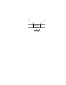
Figure 1: Reaction process: the entrance channel $b$ with amplitude $A^{b}_{2}$ continues through internal propagation started in the intrinsic state $|2\rangle$ driven by the non-Hermitian energy-dependent effective Hamiltonian (1) (with all excursions into continuum space included), and ends by exit from the intrinsic state $|1\rangle$ into the channel $a$ as described by the amplitude $A^{a\ast}_{1}(E)$.

The same transition amplitudes and propagation via intrinsic space drive the process shown schematically in Fig. 1.

The poles of the transition matrix and related full scattering matrix $S=1-2\pi iT$ are the eigenvalues of Eq. (3) located in the lower part of the complex energy plane. The reaction theory is fully consistent with resonant description in Sec. 2. However, complexity of the many-body propagator in Eq. (4) with numerous poles, interfering paths and energy dependence can make the observable cross section which is a projection of poles onto a real energy axis quite different from a collection of individual resonance peaks.

The solution of Eq. (3) with the large scale many-body Hamiltonian is a complicated task as extensively discussed in Refs. [4]. The calculation of the transition matrix (4) and of the cross section is yet another technical problem. The direct approach involving matrix inversion at all energies is extremely difficult and time consuming given large dimensions involved. The sharp resonances typically present in the spectrum make the process numerically unstable and require dense energy sampling to achieve a reasonable cross section curve. Absence of absolute numerical precision leads to instability near stable states embedded in the continuum where decays are prohibited by symmetry considerations. This problem is particularly troublesome within the $m$-scheme shell model approach. To overcome these difficulties, an alternative method has been developed which is discussed below.

3.1 Unitarity and $R$-matrix

The transition matrix (4) with the dimensionality equal to the number of open channels can be written as $T={\bf A}^{\dagger}{\cal G}{\bf A}$, where the full effective Green’s function ${\cal G}(E)={1}/({E-{\cal H}})$ includes the loss of probability into all decay channels. The factorized form of the non-Hermitian part $W=2\pi{\bf A}{\bf A}^{\dagger}$ in Eq. (1), where ${\bf A}$ represents a channel matrix (a set of columns of vectors $A^{c}_{1}$ for each channel $c$) is the key for unitarity of the $S$ matrix [10]. As shown in [11], the simple iteration of the Dyson equation using the definitions ${\cal H}=H-iW/2$ and $G=(E-H)^{-1}$ leads to the following transition and scattering matrices

$$T=\frac{R}{1+i\pi R}\,,\quad S=\frac{1-i\pi R}{1+i\pi R},$$ (5)

where the matrix $R={\bf A}^{\dagger}G{\bf A}$ is analogous to the $R$-matrix of standard reaction theory; it is based on the Hermitian part of the Hamiltonian $H=H_{0}+\Delta$ and computed as a function of energy using Chebyshev polynomial expansion in Sec. 3.2.

3.2 Time evolution of the system and Green’s function

The technique behind the Green’s function calculation in the CoSMo extends the idea suggested in [12] where densities of states in molecular systems were computed using the Chebyshev polynomial expansion of the time-dependent evolution operator.

First, the finite Hamiltonian matrix is rescaled and shifted by a constant so that the spectrum is mapped onto a generic energy interval [-1,1] using $H\rightarrow(H-E_{+})/{E_{-}}.$ The procedure involves scaling $E_{-}$ and shifting $E_{+}$ parameters, $E_{\pm}=(E_{\rm max}\pm E_{\rm min})/2$, that are determined by the upper and lower edges of the original spectrum $E_{\rm max}$ and $E_{\rm min}$, respectively. Even within the traditional Lanczos diagonalization, the rescaling, although not required, is useful for providing numerical stability. Given a trivial nature of the rescaling procedure and its reversal, below we do not introduce special notations for the rescaled Hamiltonian.

The energy representation of the retarded propagator is given by the usual Fourier image of the evolution operator,

$${G}(E)=\frac{1}{E-H}=-i\int_{0}^{\infty}dt\,\exp(iEt)\exp(-iHt),$$ (6)

where ${H}$ is the Hamiltonian operator with a negative-definite infinitesimal imaginary part. The expansion factorizes the evolution operator using the Chebyshev polynomials as follows:

$$\exp(-iHt)=\sum_{n=0}^{\infty}\,(-i)^{n}(2-\delta_{n0})\,J_{n}(t)\,T_{n}(H),$$ (7)

where $J_{n}(t)$ is the usual Bessel function and the Chebyshev polynomials are defined as $T_{n}[\cos(\theta)]=\cos(n\theta).$ In comparison to the Taylor expansion or other methods evaluating the Green’s function, the Chebyshev polynomials provide a complete set of orthogonal functions covering uniformly the interval [-1,1]. Although individual states can be resolved, the procedure is most effective when a significant energy region is involved, namely for overlapping resonances. The asymptotic of the Bessel functions assures convergence of the series. The “angle addition” equations that follow from the definition of polynomials,

$$2T_{n}(x)T_{m}(x)=T_{n+m}(x)+T_{n-m}(x)\,,\quad n\geq m,$$ (8)

are useful for the successive evaluation of series of vectors $|\lambda_{n}\rangle=T_{n}(H)|\lambda\rangle$ using the following iterative procedure:

$$|\lambda_{0}\rangle=|\lambda\rangle,\quad|\lambda_{1}\rangle=H|\lambda\rangle,\quad\text{and}\,\,\,|\lambda_{n+1}\rangle=2H|\lambda_{n}\rangle-|\lambda_{n-1}\rangle.$$ (9)

In the CoSMo approach the calculations of reactions are performed using the Fast Fourier Transformation of Eq. (6), where the expectation value of the evolution operator in (7) is computed using iterative matrix-vector multiplications (9). In this way the $R$-matrix is computed which is then used to determine the cross section (5). The Chebyshev polynomials are divergent in the complex plane; therefore only the Hermitian part $H=H_{0}+\Delta$ corresponding to the $R$ matrix can be used in the evolution operator (7). Using a conservative estimate it can be shown that $n$ iterations lead to the energy resolution $4E_{-}/n$. Unlike the reorthogonalization problem in the Lanczos algorithm, lack of numerical precision in successive matrix vector multiplication does not leads to significant deterioration of the result. $n=1024$ was typically used for CoSMo calculations.

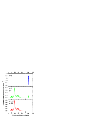
Figure 2: Strength function of a dipole operator. Upper plot: effective charges for protons and neutrons are selected equal leading to a pure isospin $T=0$ CM operator; only the CM states with energies around 100 MeV have non-zero strength. Middle plot: effective charges are selected as -1 and +1 for neutrons and protons, respectively, the resulting mixed operator shows strength in both CM and non-CM states. Lower plot: the effective charges are selected as $e_{n}=-N/A=-0.4$ and $e_{p}=Z/A=0.6$, which for ²⁰O excludes CM component from the dipole operator; the resulting strength shows no CM excitation.

3.3 Center-of-mass separation

To illustrate the effectiveness of the method, we make a digression from decays and continuum and discuss a stable large-scale shell model example of the center-of-mass (CM) problem. In Fig. 2 we show the strength function of the dipole operator. The strength function for a state $|\lambda\rangle$ is defined as

$$F_{\lambda}(E)=\langle\lambda|\delta(E-H)|\lambda\rangle=-\frac{1}{\pi}\,{\rm Im}\,\langle\lambda|G(E)|\lambda\rangle.$$ (10)

For the Hamiltonian $H$ here, we consider the full $s-p-sd-pf$ shell model space with positive parity states restricted to the $sd$ shell, while the negative parity states include all one-particle-hole excitations from the $sd$ shell. The two-body interaction is chosen as WBP [13]. A Lawson technique is used to address the CM problem with an artificial CM vibration Hamiltonian included into $H$ with a large scaling factor. As a result, all states that correspond to the CM excitations appear at high energy, around 100 MeV in our example. The strength function of the dipole operator ${D}=\sum_{a}e_{a}r_{a}$ is considered, where $e_{a}$ is the effective charge of a particle $a$. In Fig. 2 the dipole strength for excitations from the $0^{+}$ ground state of ²⁰O is plotted, namely Eq. (10) is evaluated with $|\lambda_{D}\rangle=D|{\rm g.s}\rangle.$ Depending on the choice of the effective charges for protons and neutrons, the operator $D$ can be changed from the pure CM operator to the isovector operator containing no CM component. The change in strength of CM states is shown in Fig. 2.

4 Helium isotopes

We conclude with a realistic example of CoSMo application to the chain of helium isotopes ⁴He to ¹⁰He that serves as an illustration of all techniques combined. The internal space of this simplified model contains two single-particle levels $p_{3/2}$ and $p_{1/2}$ on top of the $\alpha$-particle core. The sensitivity of the decay amplitudes $A_{1}^{c}$ to the location of thresholds and to the parent-daughter structural relations lead to the necessity of considering the entire isotope chain. The effective shell model interactions were taken from [14, 15]. These interactions are experimentally adjusted; thus it is assumed that the Hermitian renormalizations due to virtual particle excitations into continuum, $\Delta(E)$, Eq. (2), are already implicitly included; the energy dependence of $\Delta(E)$ is neglected. The diagonalization of the Hermitian many-body Hamiltonian within this valence space provides a conventional shell model solution.

One-body decays are accounted for in the model through the single-particle decay amplitudes defined as

$$A^{c}_{1}(E)=a_{j}(\epsilon)\,\,\langle 1;N|b^{\dagger}_{j}|\alpha;N-1\rangle.$$ (11)

These amplitudes correspond to a single particle amplitude $a_{j}$ of the decay leaving a residual $N-1$ nucleon state $\alpha$, while the remaining nucleons can be seen as spectators. The amplitude $a_{j}$ as a function of energy is determined with the use of the Woods-Saxon potential that models the single-particle interaction between bound and continuum states. The parameters of the potential are adjusted in order to adequately represent the ⁴He+$n$ scattering.

The two-body decays can be separated into sequential and direct ones. The sequential decays represent higher order processes generated by the same single-particle mechanism modeled here by the Woods-Saxon potential. The direct decay requires introduction of new parameters describing instantaneous removal of an interacting pair. The model includes simplest two-body terms, see further discussion in [4].

In Fig. 3 the results of calculations are shown and compared to the experimental data [16, 17, 18]. The resonance states computed according to the Breit-Wigner definition are shown with discrete lines labeled with spin, parity and decay width. The same Fig. 3 contains a separate cross section calculation which implements techniques discussed in Secs. 3.1 and 3.2. The reaction calculation is performed with the use of the same Hamiltonian (1) and thus provides an important complementary picture to the resonant structure. The cross section shown is that for elastic neutron scattering off the ground state of the $N-1$ nucleus.

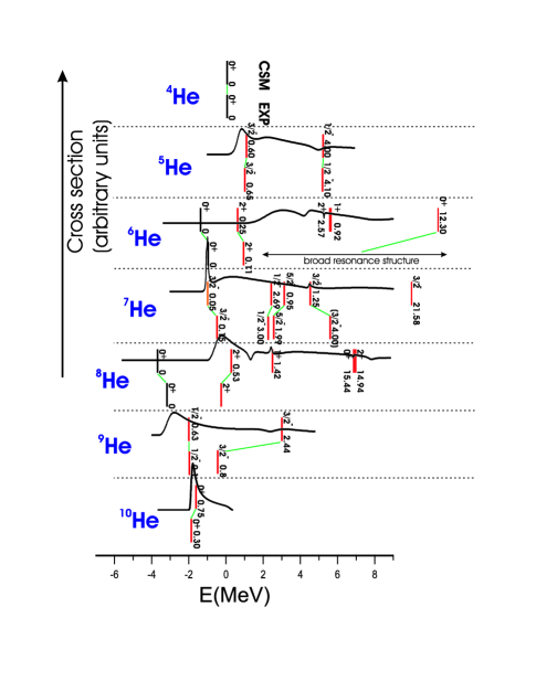
Figure 3: (Color online) CoSMo results for He isotopes. The states in the chain of isotopes starting from ⁴He (top) up to ¹⁰He (bottom) are shown as a function of the energy relative to ⁴He. The horizontal dotted lines separate isotopes. For each case, the states from CoSMo are shown above experimentally observed states. The decay width (in units of MeV) along with spin and parity is shown for each state. The solid lines above CoSMo states show the elastic neutron scattering cross section from the spin polarized state of $N-1$ isotope in the magnetic substate with $M=0$ (even) or $M=1/2$ (odd mass) quantum number.

The model, in agreement with experiment, predicts ground states of ^4,6,8He to be particle-bound. The energies of these states by construction of the model exactly agree with the prediction of the traditional shell model. The states in the continuum are approached from two perspectives, via the solution of Eq. (3) under the Breit-Wigner resonance condition and by directly plotting the cross section curve. The resonance centroids are shown with discrete lines with corresponding widths indicated. The continuum coupling changes the structure of internal states leading to resonant energies being in general different from those from the shell model prediction. The resonant patterns indirectly reveal information about structure of the states and dominant decay modes. The results for ⁷He isotope agree with recent experiments [17, 18]. Our results support the “unusual structure” of the $5/2^{-}$ state identified by [18]. Due to its relatively high spin, this state, unlike the neighboring $1/2^{-}$ state, decays mainly to the $2^{+}$ excited state in ⁶He.

The comparison of the cross section curve with discrete resonances provides a transparent picture revealing both usefulness and limitations of the resonant parameterization approach. The scattering cross sections start from thresholds set here by the ground state of the previous ($N-1$) nucleus. The cross sections at sharp resonances, such as the ground state of ⁷He, agree well with the resonance parameterization. However, generally the cross section curves are not symmetric and do not show a simple, Gaussian or Lorentzian, shape. The shape of low-lying states with widths big enough to reach threshold is particularly influenced. The association of the cross section peaks with the location of the resonance is ambiguous. A remarkable example is the case of $1/2^{-}$ state in ⁷He. The Breit-Wigner approach predicts an almost 3 MeV wide resonance at 2.3 MeV of excitation energy. The cross section curve, however, is only weakly influenced by such a deep pole and peaks near low energies reflecting primarily a proximity of threshold. This comparison of cross section and resonance parameterization may shed light onto the experimental controversy discussed in [17, 18, 19, 20].

References

- [1] H. Feshbach, Ann. Phys. 5, p. 357 (1958); 19, p. 287 (1962).
- [2] C. Mahaux and H. Weidenmüller, Shell-model approach to nuclear reactions (North-Holland Pub. Co., Amsterdam, London, 1969).
- [3] I. Rotter, Rep. Prog. Phys. 54, p. 635 (1991).
- [4] A. Volya and V. Zelevinsky, Phys. Rev. C 67, p. 54322 (2003); Phys. Rev. Lett. 94, p. 052501 (2005).
- [5] R. I. Betan, R. J. Liotta, N. Sandulescu and T. Vertse, Phys. Rev. Lett. 89, p. 042501 (2002).
- [6] N. Michel, et al., Phys. Rev. Lett. 89, p. 042502 (2002); Phys. Rev. C 67, p. 054311 (2003); Phys. Rev. C 70, p. 064313 (2004).
- [7] J. Okolowicz, M. Ploszajczak and I. Rotter, Phys. Rep. 374, p. 271 (2003).
- [8] A. F. J. Siegert, Phys. Rev. 56, p. 750 (1939).
- [9] G. Breit and E. Wigner, Phys. Rev. 49, p. 519 (1936).
- [10] L. Durand, Phys. Rev. D 14, p. 3174 (1976).
- [11] V. Sokolov and V. Zelevinsky, Nucl. Phys. A504, p. 562 (1989).
- [12] T. Ikegami and S. Iwata, J. Comput. Chem. 23, p. 310 (2002).
- [13] B. Brown, Prog. Part. Nucl. Phys. 47, p. 517 (2001).
- [14] S. Cohen and D. Kurath, Nucl. Phys. A73, p. 1 (1965).
- [15] J. Stevenson, et al., Phys. Rev. C 37, p. 2220 (1988).
- [16] Evaluated nuclear structure data file http://www.nndc.bnl.gov.
- [17] G. V. Rogachev, et al. Phys. Rev. Lett. 92, p. 232502 (2004).
- [18] A. A. Korsheninnikov et al., Phys. Rev. Lett. 82, 3581 (1999).
- [19] A. Wuosmaa et al., Phys. Rev. C 72, p. 061301(R) (2005).
- [20] M. Meister et al., Phys. Rev. Lett. 88, p. 102501 (2002).