Conserved electromagnetic currents in a relativistic optical model

Abstract

A simple model of a relativistic optical model is constructed by reducing the three-body Bethe-Salpeter equation to an effective two-body optical model. A corresponding effective current is derived for use with the optical-model wave functions. It is shown that this current satisfies a Ward-Takahashi identity involving the optical potential which results in conserved current matrix elements.

I Introduction

Dirac optical models are widely used in analyzing electron scattering data for $(e,e^{\prime})$ and $(e,e^{\prime}p)$ reactionsPVOW85 ; PVO87 ; PVO89 ; CPVO89a ; CPVO89b ; CP92 ; JOW92 ; JO ; KW97 ; KW99 ; KW03 ; USMGC93 ; USMGC95 ; USMGC96 ; UCMAD99 ; UV00 ; UCMVE01 ; MCDMU04 ; VMCMU04 ; MLJRVU06 ; MGP01a ; MGP01b ; MGP02 ; MCGP03 . Recently these models have shown to give excellent agreement with spin observables for ${}^{16}O(e,e^{\prime}p)$ Fissum where the behavior of the observables at large missing momentum has been attributed to dynamical relativistic effects due to “spinor distortion”. These models have also been used in the analysis of recent data for ${}^{4}He(e,e^{\prime}p)$ Dieterich ; Strauch ; Aniol for indications of medium modification of nucleons in the nuclei. Evidence for such modifications in this case relies on use of optical model calculations with and without medium modified from factors. Since the size of the difference between the calculation without medium modified form factors and the data is on the order of 5 to 10 percent, any conclusion based on this approach requires that the model calculations can be trusted to a similar level of accuracy. (It should be noted that this later effect has been described in a more traditional approach SBKMV05 by including charge exchange interactions. The choice of the parameters for are reasonable, but are not well constrained by data.)

Given the importance of the questions that are being addressed with these models, it is necessary to consider their foundations. The fundamental assumption is that the nucleon-nucleus interaction can be described in terms of a single-particle hamiltonian of the form

$$H=\frac{1}{i}\bm{\alpha}\cdot\bm{\nabla}+\beta\left[m+S_{OPT}(r,E)\right]+V_{OPT}(r,E)\,,$$ (1)

where $S_{OPT}(r,E)$ and $V_{OPT}(r,E)$ are complex, energy-dependent, scalar and vector optical potentials. This approach was first used to provide a phenomenological description of proton-nucleus elastic scatteringAC79 ; ACM79 ; ACMS81 . It was subsequently demonstrated that optical potentials derived from parameterized NN interactions in the impulse approximation provided a very good description of the spin observables for proton-nucleus elastic scattering at intermediate energies with a minimal number of parametersSMW93 ; CHMRS ; HPTT84 . It should be noted, however, that although the origins of the optical potential in nonrelativistic multiple-scattering theory have received a great deal of theoretical attention, the Dirac optical model proceeded by analogy to the nonrelativistic case without reference to a relativistic many-body theory.

Similarly, the first applications of the Dirac optical model to $(e,e^{\prime}p)$ and $(e,e^{\prime})$ reactions PVOW85 ; PVO87 ; PVO89 ; CPVO89a ; CPVO89b assumed that the necessary current matrix elements could be obtained in analogy to the nonrelativistic case with wave functions obtained from one-body Dirac equations and the current operator described by a one-body current. In both the nonrelativistic and relativistic cases this assumption leads to a lack of current conservation. This lack of current conservation is a direct result of the underlying many-body nature of these reactions. This manifests itself in several related ways. The first is associated with the composite nature of the nucleon resulting in the need for form factors which interfere with the usual single-particle Ward-Takahashi identities and imply that one-body current be of a much more complicated general off-shell form. The second is associated the with the appearance of many-body exchange or interaction currents. Finally, the use of an optical potential implies that the many-body problem has been reduced to an effective two-body where the contributions of channels associated with excitation of the residual system are hidden in the optical potentials. Since these hidden channels can be excited by virtual photon absorption, a consistent treatment of the reaction requires that an effective current operator be used in place of the simple one-body current. The first source of current non-conservation has been addressed by studying the effect of various on-shell equivalent forms of the single-nucleon current on the optical model calculationsPVOW85 ; CP92 ; USMGC93 ; UV00 . This gives some rough indication of the size of violation of current conservation, but does not really address the underlying problem. The second source has been addressed by including two-body meson-exchange currents in an approximate fashionMGP02 . The problem of the effect of the reduction of the many-body problem to an effective optical model on the current has been discussed in a general fashion, but has not been studied in any concrete way.CPVO89a ; BVO90

The purpose of this paper is to show that it is indeed possible to obtain a Dirac optical model from an underlying covariant theory and to obtain the corresponding effective current operator necessary to maintain electromagnetic current conservation. In doing this several choices will be made in the reorganization of the covariant theory into the optical model. Clearly, this approach is not necessarily unique. Therefore, the hope is that this work will stimulate the development of alternate approaches with the hope that this will lead to an improvement in the phenomenology for the application of the Dirac optical model to electromagnetic processes.

The starting point for this work are the many-body Bethe-Salpeter equations. These equations are most easily understood as a resummation of all Feynman diagrams for n-point functions. The $n/2$ particles associated with the external legs of the n-point function are treated as explicit degrees of freedom while all other degrees of freedom are collected into a set of irreducible kernels. These degrees of freedom are implicit. The kernels are then used in integral equations to sum all contributions to the n-point functions. Since these equations are based in Feynman perturbation theory, all elements of the integral equations are manifestly covariant. For spin-1/2 constituents the one-body propagators appearing in the integral equations are solutions to the Dirac equation so it reasonable to believe that it is be possible to reduce the many-body problem to an effective theory involving the interaction of a Dirac particle with an $(n-1)$-body system. The structure of the integral equation for the Bethe-Salpeter $n$-point functions is similar in form to those for nonrelativistic multiple-scattering theory with the exceptions that all integrals are four-dimensional rather than three dimensional, and that the all propagators are local, whereas propagators of time-ordered description usually used in multiple-scattering theory are global.

For simplicity, the simplest illustrative case of the process, the three-body Bethe-Salpeter equationTaylor66 ; norm for distinguishable particles, is used to show how the reduction to an effective optical model can be implemented. This equation is relatively simple in structure and the construction of electromagnetic current matrix elements for this equation is well understoodkb97II ; kb99 ; 3NCur . The optical model is obtained by reducing the three-body problem to an effective two-body problem. The effective kernel for the interaction between the bound state of two of the particles and the remaining particle can then be interpreted as an “optical potential.” A similar reduction of the Bethe-Salpeter current matrix elements leads to the identification of an effective current operator consistent with the optical model. This optical model current will be shown to result in conserved current matrix elements.

In the first section the optical model for the interaction of one particle with a bound state of the remaining pair is constructed. Next, bound and scattering states are defined in terms of the optical model states. Finally, the effective optical model current is constructed and the impulse approximation contribution to the effective current is isolated. It is then shown that the optical model current satisfies a Ward-Takahashi identity involving the optical potential which results in conserved current matrix elements.

II Optical Model Representation of the Three-body Scattering Matrix

Here we will use a matrix form for the three-body Bethe-Salpeter equation described in 3NCur to simplify the reduction of the three-body problem to the effective two-body problem. This is formulation is summarized in the appendix for the convenience of the reader. For three distinguishable particles, the three-body scattering matrix can be written in matrix form as using (76)

$$\bm{{\cal T}}=\bm{{\cal M}}-\bm{{\cal M}}\bm{G}^{0}_{BS}\bm{{B}}\bm{{\cal T}}\,,$$ (2)

where the matrices are defined in the appendix.

Our objective is to reduce this expression so than we can extract an effective equation for particle 1 scattering from a bound state of particles 2 and 3. This is accomplished by separating the two-body t matrix for particles 2 and 3 into terms containing bound-state poles and a residual piece containing only the scattering cuts. Assuming that there is only a single bound state for particles 2 and 3, the two-body scattering matrix in momentum space has the form

$$M^{1}(p^{1\prime},p^{1},P^{1}) = \frac{1}{2E(\bm{P})}\left(\frac{\Gamma^{(2)1}(p^{1\prime},\hat{P}^{1}){\Gamma^{(2)1}}^{\dagger}(p^{1},\hat{P}^{1})}{{P^{1}}^{0}-E(\bm{P}^{1})+i\eta}-\frac{\Gamma^{(2)1}(-p^{1\prime},-\hat{P}^{1}){\Gamma^{(2)1}}^{\dagger}(-p^{1},-\hat{P}^{1})}{{P^{1}}^{0}+E(\bm{P}^{1})-i\eta}\right)$$ (3)

$$+M^{1}_{r}(p^{1\prime},p^{1},P^{1})\,,$$

where $P^{1}$ is the total four-momentum of the pair, $p^{1}$ and $p^{1\prime}$ are the initial and final relative four-momenta of the pair, $\Gamma^{(2)1}$ is the bound-state vertex function for the pair, $m^{1}$ is the mass of the bound state and $M^{1}_{r}$ is the residual scattering matrix. For relativistic many-body equations there is no clean factorization of the vertex functions into relative and center-of-mass pieces. This means that vertex functions are explicitly dependent upon the total momentum. Any spinor indices associate with the vertex function are suppressed and are assumed to be summed. Note that there are positive and negative poles associated with the positive- and negative-energy bound states. There are several ways to precede at this point in reducing the three-body problem to an effective two-body problem. Both the positive and negative poles can be retained and thus explicitly include the interaction with particle 1 and the negative-energy bound state. This has the virtue that the decomposition of the scattering matrix can be written in a manifestly covariant form. However, any attempt to write this in the form of an optical model will result in a form which is more complicated than is usually assumed. In addition, it is reasonable to assume that the contributions from the negative-energy pole will be small especially when this approach is extended to systems with more particles which means that the additional complexity may have little real physical impact.

A second approach would then be to treat only the positive-energy pole with the negative energy pole becoming part of the residual scattering matrix. This decomposition will not be manifestly covariant. Furthermore, the vertex functions are only uniquely defined at the pole and (3) assumes that they are defined at this point as is indicated by the hat over the total momentum. The momenta in (2) are not similarly restricted and the action of inverse two-body propagators on the bound state are not generally defined.

A third alternative, which is the one used here, is to assume that in any loop integrals involving the bound state the positive energy pole will be picked up resulting which will restrict $P^{1}$ to be on-shell. This prescription is manifestly covariant and the resulting decomposition of the two-body scattering matrix is also covariant. This can be realized in the equations for the three-body scattering matrix by writing

$$\bm{{\cal M}}=-\bm{D}^{1}\left|\Gamma^{(2)1}\right>iG_{1}^{-1}(i{\cal Q}^{1})\left<\Gamma^{(2)1}\right|{\bm{D}^{1}}^{T}+\bm{{\cal M}}_{R}=\bm{{\cal M}}_{P}+\bm{{\cal M}}_{R}\,,$$ (4)

where

$$\bm{D}^{1}=\left(\begin{array}[]{c}0\\ 1\\ 0\\ 0\end{array}\right)$$ (5)

and ${\cal Q}^{1}$ is an operator that places the total momentum for particles 2 and 3 on the bound-state mass shell by requiring that the appropriate pole be picked up in any loops containing the two-body t-matrix for particles 2 and 3.

We can now decompose the equation for the t-matrix according to whether the initial (final) interaction is the pole contribution (superscript $P$) or the residual contribution (superscript $R$.) This leads to the set of coupled matrix equations

$$\bm{{\cal T}}^{PP} = \bm{{\cal M}}_{P}-\bm{{\cal M}}_{P}\bm{G}^{0}_{BS}\bm{{B}}\left(\bm{{\cal T}}^{PP}+\bm{{\cal T}}^{RP}\right)$$ (6)

$$\bm{{\cal T}}^{RP} = -\bm{{\cal M}}_{R}\bm{G}^{0}_{BS}\bm{{B}}\left(\bm{{\cal T}}^{PP}+\bm{{\cal T}}^{RP}\right)$$ (7)

$$\bm{{\cal T}}^{PR} = -\bm{{\cal M}}_{P}\bm{G}^{0}_{BS}\bm{{B}}\left(\bm{{\cal T}}^{PR}+\bm{{\cal T}}^{RR}\right)$$ (8)

$$\bm{{\cal T}}^{RR} = \bm{{\cal M}}_{R}-\bm{{\cal M}}_{R}\bm{G}^{0}_{BS}\bm{{B}}\left(\bm{{\cal T}}^{PR}+\bm{{\cal T}}^{RR}\right)\,.$$ (9)

The solution of this set of equations is facilitated by defining a scattering matrix that does not contain any contributions from the bound state for particles 2 and 3. This is defined as

$$\bm{T}_{R}=\bm{{\cal M}}_{R}-\bm{{\cal M}}_{R}\bm{G}^{0}_{BS}\bm{{B}}\bm{T}_{R}=\bm{{\cal M}}_{R}-\bm{T}_{R}\bm{G}^{0}_{BS}\bm{{B}}\bm{{\cal M}}_{R}\,.$$ (10)

The second of these two forms can be solved to give

$$\bm{{\cal M}}_{R}=\bm{T}_{R}+\bm{T}_{R}\bm{G}^{0}_{BS}\bm{{B}}\bm{{\cal M}}_{R}\,.$$ (11)

Using this, (7) can be rewritten as

$$\bm{{\cal T}}^{RP} = -\left(\bm{T}_{R}+\bm{T}_{R}\bm{G}^{0}_{BS}\bm{{B}}\bm{{\cal M}}_{R}\right)\bm{G}^{0}_{BS}\bm{{B}}\left(\bm{{\cal T}}^{PP}+\bm{{\cal T}}^{RP}\right)$$ (12)

$$= -\bm{T}_{R}\bm{G}^{0}_{BS}\bm{{B}}\left(\bm{{\cal T}}^{PP}+\bm{{\cal T}}^{RP}\right)-\bm{T}_{R}\bm{G}^{0}_{BS}\bm{{B}}\bm{{\cal M}}_{R}\bm{G}^{0}_{BS}\bm{{B}}\left(\bm{{\cal T}}^{PP}+\bm{{\cal T}}^{RP}\right)$$

$$= -\bm{T}_{R}\bm{G}^{0}_{BS}\bm{{B}}\left(\bm{{\cal T}}^{PP}+\bm{{\cal T}}^{RP}\right)+\bm{T}_{R}\bm{G}^{0}_{BS}\bm{{B}}\bm{{\cal T}}^{RP}$$

$$= -\bm{T}_{R}\bm{G}^{0}_{BS}\bm{{B}}\bm{{\cal T}}^{PP}\,,$$

where we have used the fact that ${\bm{D}^{1}}^{T}\bm{B}\bm{D}^{1}=0$ in simplifying the equations. This can be used in (6) to give

$$\bm{{\cal T}}^{PP}=\bm{{\cal M}}_{P}-\bm{{\cal M}}_{P}\bm{G}^{0}_{BS}\bm{{B}}\bm{{\cal T}}^{RP}=\bm{{\cal M}}_{P}+\bm{{\cal M}}_{P}\bm{G}^{0}_{BS}\bm{{B}}\bm{T}_{R}\bm{G}^{0}_{BS}\bm{{B}}\bm{{\cal T}}^{PP}\,.$$ (13)

From (4),

$$\bm{{\cal M}}_{P}=-\bm{D}^{1}\left|\Gamma^{(2)1}\right>iG_{1}^{-1}(i{\cal Q}^{1})\left<\Gamma^{(2)1}\right|{\bm{D}^{1}}^{T}=-iG_{1}^{-1}\bm{D}^{1}\left|\Gamma^{(2)1}\right>(-iG_{1})i{\cal Q}^{1}\left<\Gamma^{(2)1}\right|{\bm{D}^{1}}^{T}iG_{1}^{-1}\,.$$ (14)

Using this and iterating of (13) it is possible to make the conjecture that

$$\bm{{\cal T}}^{PP}=-iG_{1}^{-1}\bm{D}^{1}\left|\Gamma^{(2)1}\right>i{\cal Q}^{1}(-iG_{OPT})i{\cal Q}^{1}\left<\Gamma^{(2)1}\right|{\bm{D}^{1}}^{T}iG_{1}^{-1}\,.$$ (15)

Substituting this into (13),

$$-iG_{1}^{-1}\bm{D}^{1}\left|\Gamma^{(2)1}\right>i{\cal Q}^{1}(-iG_{OPT})i{\cal Q}^{1}\left<\Gamma^{(2)1}\right|{\bm{D}^{1}}^{T}iG_{1}^{-1}$$

$$\qquad=-iG_{1}^{-1}\bm{D}^{1}\left|\Gamma^{(2)1}\right>(-iG_{1})i{\cal Q}^{1}\left<\Gamma^{(2)1}\right|{\bm{D}^{1}}^{T}iG_{1}^{-1}$$

$$\qquad+iG_{1}^{-1}\bm{D}^{1}\left|\Gamma^{(2)1}\right>(-iG_{1})i{\cal Q}^{1}\left<\Gamma^{(2)1}\right|{\bm{D}^{1}}^{T}iG_{1}^{-1}\bm{G}^{0}_{BS}\bm{{B}}\bm{T}_{R}\bm{G}^{0}_{BS}\bm{{B}}iG_{1}^{-1}\bm{D}^{1}\left|\Gamma^{(2)1}\right>i{\cal Q}^{1}$$

$$\qquad\times(-iG_{OPT})i{\cal Q}^{1}\left<\Gamma^{(2)1}\right|{\bm{D}^{1}}^{T}iG_{1}^{-1}\,.$$ (16)

We can then identify

$$i{\cal Q}^{1}G_{OPT}i{\cal Q}^{1} = G_{1}i{\cal Q}^{1}$$ (17)

$$-G_{1}i{\cal Q}^{1}\left<\Gamma^{(2)1}\right|{\bm{D}^{1}}^{T}iG_{1}^{-1}\bm{G}^{0}_{BS}\bm{{B}}\bm{T}_{R}\bm{G}^{0}_{BS}\bm{{B}}iG_{1}^{-1}\bm{D}^{1}\left|\Gamma^{(2)1}\right>i{\cal Q}^{1}G_{OPT}i{\cal Q}^{1}$$

$$= G_{1}i{\cal Q}^{1}-G_{1}i{\cal Q}^{1}\left<\Gamma^{(2)1}\right|{\bm{D}^{1}}^{T}G^{1}_{BS}\bm{{B}}\bm{T}_{R}G^{1}_{BS}\bm{{B}}\bm{D}^{1}\left|\Gamma^{(2)1}\right>{\cal Q}^{1}G_{OPT}i{\cal Q}^{1}$$

where $G^{1}_{BS}=-iG_{2}G_{3}$ is the free two-body propagator for particles 2 and 3, and $\left|\Phi^{(2)1}\right>=G^{1}_{BS}\left|\Gamma^{(2)1}\right>$ is the bound-state Bethe-Salpeter wave function for particles 2 and 3. Defining

$$V_{OPT}=i{\cal Q}^{1}\left<\Phi^{(2)1}\right|{\bm{D}^{1}}^{T}\bm{{B}}\bm{T}_{R}\bm{{B}}\bm{D}^{1}\left|\Phi^{(2)1}\right>{\cal Q}^{1}$$ (18)

as the optical potential, the optical model propagator can be rewritten as

$$i{\cal Q}^{1}G_{OPT}i{\cal Q}^{1}=\left(G_{1}-G_{1}V_{OPT}G_{OPT}\right)i{\cal Q}^{1}\,.$$ (19)

Note that keeping only the leading terms in 18 yields

$$V_{OPT}=i{\cal Q}^{1}\left<\Phi^{(2)1}\right|\left({\cal M}^{0}+{\cal M}^{2}+{\cal M}^{3}\right)\left|\Phi^{(2)1}\right>{\cal Q}^{1}\,.$$ (20)

With the exception of the explicit three-body term ${\cal M}^{0}$, this is the impulse approximation to the optical potential.

Substituting (11) into (9) gives

$$\bm{{\cal T}}^{RR} = \bm{T}_{R}+\bm{T}_{R}\bm{G}^{0}_{BS}\bm{{B}}\bm{{\cal M}}_{R}-\left(\bm{T}_{R}+\bm{T}_{R}\bm{G}^{0}_{BS}\bm{{B}}\bm{{\cal M}}_{R}\right)\bm{G}^{0}_{BS}\bm{{B}}\left(\bm{{\cal T}}^{PR}+\bm{{\cal T}}^{RR}\right)$$ (21)

$$= \bm{T}_{R}+\bm{T}_{R}\bm{G}^{0}_{BS}\bm{{B}}\bm{{\cal M}}_{R}-\bm{T}_{R}\bm{G}^{0}_{BS}\bm{{B}}\left(\bm{{\cal T}}^{PR}+\bm{{\cal T}}^{RR}\right)$$

$$\qquad-\bm{T}_{R}\bm{G}^{0}_{BS}\bm{{B}}\bm{{\cal M}}_{R}\bm{G}^{0}_{BS}\bm{{B}}\left(\bm{{\cal T}}^{PR}+\bm{{\cal T}}^{RR}\right)$$

$$= \bm{T}_{R}+\bm{T}_{R}\bm{G}^{0}_{BS}\bm{{B}}\bm{{\cal M}}_{R}-\bm{T}_{R}\bm{G}^{0}_{BS}\bm{{B}}\left(\bm{{\cal T}}^{PR}+\bm{{\cal T}}^{RR}\right)+\bm{T}_{R}\bm{G}^{0}_{BS}\bm{{B}}\left(\bm{{\cal T}}^{RR}-\bm{{\cal M}}_{R}\right)$$

$$= \bm{T}_{R}-\bm{T}_{R}\bm{G}^{0}_{BS}\bm{{B}}\bm{{\cal T}}^{PR}\,.$$

This can be used in (8) to yield

$$\bm{{\cal T}}^{PR} = -\bm{{\cal M}}_{P}\bm{G}^{0}_{BS}\bm{{B}}\bm{{\cal T}}^{RR}$$ (22)

$$= -\bm{{\cal M}}_{P}\bm{G}^{0}_{BS}\bm{{B}}\left(\bm{T}_{R}-\bm{T}_{R}\bm{G}^{0}_{BS}\bm{{B}}\bm{{\cal T}}^{PR}\right)$$

$$= -\bm{{\cal M}}_{P}\bm{G}^{0}_{BS}\bm{{B}}\bm{T}_{R}+\bm{{\cal M}}_{P}\bm{G}^{0}_{BS}\bm{{B}}\bm{T}_{R}\bm{G}^{0}_{BS}\bm{{B}}\bm{{\cal T}}^{PR}$$

Iteration of this shows that that it can be rewritten as

$$\bm{{\cal T}}^{PR}=-\bm{{\cal T}}^{PP}\bm{G}^{0}_{BS}\bm{{B}}\bm{T}_{R}\,.$$ (23)

Using (23) in (21),

$$\bm{{\cal T}}^{RR}=\bm{T}_{R}+\bm{T}_{R}\bm{G}^{0}_{BS}\bm{{B}}\bm{{\cal T}}^{PP}\bm{G}^{0}_{BS}\bm{{B}}\bm{T}_{R}\,.$$ (24)

The complete t-matrix is the sum of (12), (13), (23) and (24). This can be written as

$$\bm{{\cal T}} = \bm{{\cal T}}^{PP}+\bm{{\cal T}}^{RP}+\bm{{\cal T}}^{PR}+\bm{{\cal T}}^{RR}$$ (25)

$$= \bm{{\cal T}}^{PP}-\bm{T}_{R}\bm{G}^{0}_{BS}\bm{{B}}\bm{{\cal T}}^{PP}-\bm{{\cal T}}^{PP}\bm{G}^{0}_{BS}\bm{{B}}\bm{T}_{R}+\bm{T}_{R}+\bm{T}_{R}\bm{G}^{0}_{BS}\bm{{B}}\bm{{\cal T}}^{PP}\bm{G}^{0}_{BS}\bm{{B}}\bm{T}_{R}$$

$$= \bm{T}_{R}+\left(\bm{1}-\bm{T}_{R}\bm{G}^{0}_{BS}\bm{{B}}\right)\bm{{\cal T}}^{PP}\left(\bm{1}-\bm{G}^{0}_{BS}\bm{{B}}\bm{T}_{R}\right)\,.$$

III Wave Functions

We also need a similar separation for the scattering state of particle 1 with the bound state of particles 2 and 3 and for the three-body bound state. To obtain the former, consider the left-handed propagator defined by (78). Using (25), this can be rewritten as

$$\bm{{\cal G}}_{L} = \bm{{G}}^{0}_{BS}-\bm{{G}}^{0}_{BS}\left(\bm{{1+B}}\right)\bm{{\cal T}}\bm{{G}}^{0}_{BS}$$ (26)

$$= \bm{{G}}^{0}_{BS}-\bm{{G}}^{0}_{BS}\left(\bm{{1+B}}\right)\bm{T}_{R}\bm{{G}}^{0}_{BS}$$

$$\quad-\bm{{G}}^{0}_{BS}\left(\bm{{1+B}}\right)\left(\bm{1}-\bm{T}_{R}\bm{G}^{0}_{BS}\bm{{B}}\right)\bm{{\cal T}}^{PP}\left(\bm{1}-\bm{G}^{0}_{BS}\bm{{B}}\bm{T}_{R}\right)\bm{{G}}^{0}_{BS}$$

$$= \bm{{G}}^{0}_{BS}-\bm{{G}}^{0}_{BS}\left(\bm{{1+B}}\right)\bm{T}_{R}\bm{{G}}^{0}_{BS}$$

$$\quad-\bm{{G}}^{0}_{BS}\left(\bm{{1+B}}\right)\left(\bm{1}-\bm{T}_{R}\bm{G}^{0}_{BS}\bm{{B}}\right)iG_{1}^{-1}\bm{D}^{1}\left|\Gamma^{(2)1}\right>i{\cal Q}^{1}(-iG_{OPT})(i{\cal Q}^{1})$$

$$\qquad\times\left<\Gamma^{(2)1}\right|{\bm{D}^{1}}^{T}iG_{1}^{-1}\left(\bm{1}-\bm{G}^{0}_{BS}\bm{{B}}\bm{T}_{R}\right)\bm{{G}}^{0}_{BS}$$

$$= \bm{{G}}^{0}_{BS}-\bm{{G}}^{0}_{BS}\left(\bm{{1+B}}\right)\bm{T}_{R}\bm{{G}}^{0}_{BS}$$

$$\quad+i\bm{{G}}^{0}_{BS}\left(\bm{{1+B}}\right)\left(\bm{1}-\bm{T}_{R}\bm{G}^{0}_{BS}\bm{{B}}\right)iG_{1}^{-1}\bm{D}^{1}\left|\Gamma^{(2)1}\right>$$

$$\quad\times\left(G_{1}-G_{1}V_{OPT}G_{OPT}\right)i{\cal Q}^{1}\left<\Phi^{(2)1}\right|{\bm{D}^{1}}^{T}\left(\bm{1}-\bm{{B}}\bm{T}_{R}\bm{{G}}^{0}_{BS}\right)\,.$$

From the residue of the pole contribution to $G_{1}$, we can identify the scattering state as

$$\left<\bm{\Phi}^{1(-)}\right| = \left<\bm{p}_{1},\bm{P}^{1}\right|\left(1-V_{OPT}G_{OPT}\right)i{\cal Q}^{1}\left<\Phi^{(2)1}\right|{\bm{D}^{1}}^{T}\left(\bm{1}-\bm{{B}}\bm{T}_{R}\bm{{G}}^{0}_{BS}\right)$$ (27)

$$= \left<\bm{p}_{1},\bm{P}^{1}\right|\left(1-T_{OPT}G_{1}\right)i{\cal Q}^{1}\left<\Phi^{(2)1}\right|{\bm{D}^{1}}^{T}\left(\bm{1}-\bm{{B}}\bm{T}_{R}\bm{{G}}^{0}_{BS}\right)\,,$$

where $P^{1}$ is the momentum of the bound state of particles 2 and 3.

The three-body bound-state vertex function, defined by (81), can be written as

$$\left|\bm{{\Gamma}}\right>=-\bm{{\cal V}}\bm{{G}}^{0}_{BS}\left(\bm{1}+\bm{{B}}\right)\left|\bm{{\Gamma}}\right>=-\bm{{\cal M}}\bm{{G}}^{0}_{BS}\bm{{B}}\left|\bm{{\Gamma}}\right>\,.$$ (28)

Separating the vertex function into contributions where the last interaction contains either the pole in the residual parts of the scattering matrix for particles 2 and 3 gives

$$\left|\bm{{\Gamma}}_{P}\right> = -\bm{{\cal M}}_{P}\bm{{G}}^{0}_{BS}\bm{{B}}\left|\bm{{\Gamma}}\right>$$ (29)

$$\left|\bm{{\Gamma}}_{R}\right> = -\bm{{\cal M}}_{R}\bm{{G}}^{0}_{BS}\bm{{B}}\left|\bm{{\Gamma}}\right>\,.$$ (30)

Using the definition of the pole contribution,

$$\left|\bm{{\Gamma}}_{P}\right> = \bm{D}^{1}\left|\Gamma^{(2)1}\right>iG_{1}^{-1}i{\cal Q}^{1}\left<\Gamma^{(2)1}\right|{\bm{D}^{1}}^{T}\bm{{G}}^{0}_{BS}\bm{{B}}\left|\bm{{\Gamma}}\right>$$ (31)

$$= \bm{D}^{1}\left|\Gamma^{(2)1}\right>i{\cal Q}^{1}\left<\Phi^{(2)1}\right|{\bm{D}^{1}}^{T}\bm{{B}}\left|\bm{{\Gamma}}\right>\,.$$

The remaining part of the vertex function is

$$\left|\bm{{\Gamma}}_{R}\right> = -\left({\bm{T}}_{R}+\bm{T}_{R}\bm{G}^{0}_{BS}\bm{{B}}\bm{{\cal M}}_{R}\right)\bm{{G}}^{0}_{BS}\bm{{B}}\left|\bm{{\Gamma}}\right>$$ (32)

$$= -{\bm{T}}_{R}\bm{{G}}^{0}_{BS}\bm{{B}}\left|\bm{{\Gamma}}\right>-\bm{T}_{R}\bm{G}^{0}_{BS}\bm{{B}}\bm{{\cal M}}_{R}\bm{{G}}^{0}_{BS}\bm{{B}}\left|\bm{{\Gamma}}\right>$$

$$= -{\bm{T}}_{R}\bm{{G}}^{0}_{BS}\bm{{B}}\left|\bm{{\Gamma}}\right>+\bm{T}_{R}\bm{G}^{0}_{BS}\bm{{B}}\left|\bm{{\Gamma}}_{R}\right>$$

$$= -{\bm{T}}_{R}\bm{{G}}^{0}_{BS}\bm{{B}}\left|\bm{{\Gamma}}_{P}\right>$$

Using $\bm{D}^{1T}\bm{B}\bm{D}^{1}=0$ in (31), substituting $\left|\bm{{\Gamma}}_{R}\right>$ from (32) and iterating once,

$$\left|\bm{{\Gamma}}_{P}\right> = \bm{D}^{1}\left|\Gamma^{(2)1}\right>i{\cal Q}^{1}\left<\Phi^{(2)1}\right|{\bm{D}^{1}}^{T}\bm{{B}}\left|\bm{{\Gamma}}_{R}\right>$$ (33)

$$= -\bm{D}^{1}\left|\Gamma^{(2)1}\right>i{\cal Q}^{1}\left<\Phi^{(2)1}\right|{\bm{D}^{1}}^{T}\bm{{B}}{\bm{T}}_{R}\bm{{G}}^{0}_{BS}\bm{{B}}\left|\bm{{\Gamma}}_{P}\right>$$

$$= -\bm{D}^{1}\left|\Gamma^{(2)1}\right>i{\cal Q}^{1}\left<\Phi^{(2)1}\right|{\bm{D}^{1}}^{T}\bm{{B}}{\bm{T}}_{R}\bm{{G}}^{0}_{BS}\bm{{B}}\bm{D}^{1}\left|\Gamma^{(2)1}\right>i{\cal Q}^{1}\left<\Phi^{(2)1}\right|{\bm{D}^{1}}^{T}\bm{{B}}\left|\bm{{\Gamma}}\right>$$

$$= -\bm{D}^{1}\left|\Gamma^{(2)1}\right>i{\cal Q}^{1}\left<\Phi^{(2)1}\right|{\bm{D}^{1}}^{T}\bm{{B}}{\bm{T}}_{R}\bm{{B}}\bm{D}^{1}\left|\Phi^{(2)1}\right>(-iG_{1})i{\cal Q}^{1}\left<\Phi^{(2)1}\right|{\bm{D}^{1}}^{T}\bm{{B}}\left|\bm{{\Gamma}}\right>$$

$$= -i\bm{D}^{1}\left|\Gamma^{(2)1}\right>V_{OPT}(-iG_{1})\left<\Phi^{(2)1}\right|{\bm{D}^{1}}^{T}\bm{{B}}\left|\bm{{\Gamma}}\right>\,.$$

Comparing the first and last lines shows that

$${\cal Q}^{1}\left<\Phi^{(2)1}\right|{\bm{D}^{1}}^{T}\bm{{B}}\left|\bm{{\Gamma}}\right>=-V_{OPT}(-iG_{1})\left<\Phi^{(2)1}\right|{\bm{D}^{1}}^{T}\bm{{B}}\left|\bm{{\Gamma}}\right>\,,$$ (34)

which is of the form of the bound-state vertex function for the optical model.

The complete three-body vertex function can now be reconstructed using (32) and (34) to give

$$\left|\bm{{\Gamma}}\right> = \left|\bm{{\Gamma}}_{P}\right>+\left|\bm{{\Gamma}}_{R}\right>=\left(\bm{1}-{\bm{T}}_{R}\bm{{G}}^{0}_{BS}\bm{{B}}\right)\left|\bm{{\Gamma}}_{P}\right>$$ (35)

$$= \left(\bm{1}-{\bm{T}}_{R}\bm{{G}}^{0}_{BS}\bm{{B}}\right)\bm{D}^{1}\left|\Gamma^{(2)1}\right>i{\cal Q}^{1}\left<\Phi^{(2)1}\right|{\bm{D}^{1}}^{T}\bm{{B}}\left|\bm{{\Gamma}}\right>\,.$$

The Bethe-Salpeter wave function is then

$$\left|\bm{\Psi}\right>=\bm{G}^{0}_{BS}\left|\bm{{\Gamma}}\right>=\left(\bm{1}-\bm{{G}}^{0}_{BS}{\bm{T}}_{R}\bm{{B}}\right)\bm{D}^{1}\left|\Phi^{(2)1}\right>(-iG_{1})i{\cal Q}^{1}\left<\Phi^{(2)1}\right|{\bm{D}^{1}}^{T}\bm{{B}}\left|\bm{{\Gamma}}\right>$$ (36)

and

$$\Psi_{OPT}=(-iG_{1})i{\cal Q}^{1}\left<\Phi^{(2)1}\right|{\bm{D}^{1}}^{T}\bm{{B}}\left|\bm{{\Gamma}}\right>$$ (37)

can be identified as the optical model wave function.

IV Electromagnetic Current Matrix Element

At this point it is necessary to deal with a problem that is occurs in describing the current matrix element for the Bethe-Salpeter equation that is not present in the usual nonrelativistic approach. Some care must be taken with defining the Bethe-Salpeter current operator if the matrix elements are to be of the form

$${\cal J}^{\mu}=\left<\bm{\Psi}_{f}\right|\bm{J}^{\mu}\left|\bm{\Psi}_{i}\right>\,.$$ (38)

Consider the contribution from the absorption of a virtual photon on particle 1. The initial state wave function can produce a contribution described by Fig. 1a, while the final state wave function can produce a contribution described Fig. 1b. Since these are Feynman diagrams and topologically equivalent, these two diagrams give identical identical contributions and including both contributions will double count. Therefore, in order to write the matrix element element in the symmetric form (38), it is necessary to correct the current operator to correct for the double counting.

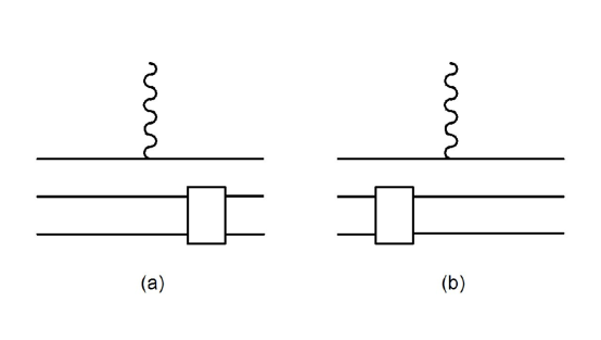
Figure 1: These Feynman diagrams represent contributions to the seven-point function. The particles are label 1 to 3 from top to bottom. The rectangles represent two-body kernels.

This can be done by replacing the one-body current by the currents represented by Fig. 2. This was pointed out in kb97II ; kb99 and is included in the definition of the Bethe-Salpeter effective current operator defined in 3NCur given by (89) and (94).

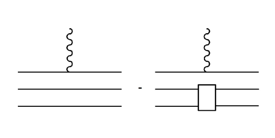
Figure 2: Feynman diagrams representing the correction to the current operator to correct for double counting.

Now consider the electromagnetic current matrix element for ejecting particle 1 from the bound state into the continuum state where particles 2 and 3 remain bound. This is

$${\cal J}^{\mu} = \left<\bm{\Phi}^{1(-)}\right|\bm{J}^{\mu}_{\rm eff}\left|\bm{\Psi}\right>$$ (39)

$$= \left<\bm{p}_{1},\bm{P}^{1}\right|\left(1-T_{OPT}(-iG_{1})\right)i{\cal Q}^{1}\left<\Phi^{(2)1}\right|{\bm{D}^{1}}^{T}\left(\bm{1}-\bm{{B}}\bm{T}_{R}\bm{{G}}^{0}_{BS}\right)\bm{J}^{\mu}_{\rm eff}$$

$$\qquad\left(\bm{1}-\bm{{G}}^{0}_{BS}{\bm{T}}_{R}\bm{{B}}\right)\bm{D}^{1}\left|\Phi^{(2)1}\right>(-iG_{1})i{\cal Q}^{1}\left<\Phi^{(2)1}\right|{\bm{D}^{1}}^{T}\bm{{B}}\left|\bm{{\Gamma}}\right>$$

$$= \left<\bm{p}_{1},\bm{P}^{1}\right|\left(1-T_{OPT}(-iG_{1})\right)J^{\mu}_{OPT}(-iG_{1})\left<\Phi^{(2)1}\right|{\bm{D}^{1}}^{T}\bm{{B}}\left|\bm{{\Gamma}}\right>\,,$$

where

$$J^{\mu}_{OPT}=i{\cal Q}^{1}\left<\Phi^{(2)1}\right|{\bm{D}^{1}}^{T}\left(\bm{1}-\bm{{B}}\bm{T}_{R}\bm{{G}}^{0}_{BS}\right)\bm{J}^{\mu}_{\rm eff}\left(\bm{1}-\bm{{G}}^{0}_{BS}{\bm{T}}_{R}\bm{{B}}\right)\bm{D}^{1}\left|\Phi^{(2)1}\right>i{\cal Q}^{1}$$ (40)

and $\bm{J}^{\mu}_{\rm eff}$ is defined by (94).

Considerable care must be taken in evaluating this expression. To simplify the derivation, we have used the operator $i{\cal Q}^{1}$ to place the bound state on shell. Operators of this type were introduced in norm and elaborated in 2NCur and 3NCur . This is a very singular operator and must be treated with extreme care. In particular this operator is not associative and its evaluation depends on its context in the evaluation of physical quantities. To see this consider the two-body scattering matrix for particles 2 and 3 given by

$$M^{1}=V^{1}-V^{1}G^{1}M^{1}=V^{1}-M^{1}G^{1}V^{1}\,.$$ (41)

The second form of this equation can be solved to give

$$V^{1}=M^{1}+M^{1}G^{1}V^{1}\,.$$ (42)

Substituting this into the first form leads to the nonlinear form of the equation for the scattering matrix

$$M^{1} = V^{1}-M^{1}G^{1}M^{1}-M^{1}G^{1}V^{1}G^{1}M^{1}=V^{1}-M^{1}G^{1}{G^{1}}^{-1}G^{1}M^{1}-M^{1}G^{1}V^{1}G^{1}M^{1}$$ (43)

$$= V^{1}-M^{1}G^{1}({G^{1}}^{-1}+V^{1})G^{1}M^{1}=V^{1}-M^{1}G^{1}{{\cal G}^{1}}^{-1}G^{1}M^{1}\,.$$

Note that since ${{\cal G}^{1}}^{-1}$ must vanish at the bound state pole, both sides of this equation have simple pole at this point. The residues of these poles give

$$-\left|\Gamma^{(2)1}\right>i{\cal Q}^{1}\left<\Gamma^{(2)1}\right|=-\left|\Gamma^{(2)1}\right>i{\cal Q}^{1}\left<\Gamma^{(2)1}\right|G^{1}{{\cal G}^{1}}^{-1}G^{1}\left|\Gamma^{(2)1}\right>i{\cal Q}^{1}\left<\Gamma^{(2)1}\right|\,.$$ (44)

This requires that

$$i{\cal Q}^{1}=i{\cal Q}^{1}\left<\Gamma^{(2)1}\right|G^{1}{{\cal G}^{1}}^{-1}G^{1}\left|\Gamma^{(2)1}\right>i{\cal Q}^{1}=i{\cal Q}^{1}\left<\Phi^{(2)1}\right|{{\cal G}^{1}}^{-1}\left|\Phi^{(2)1}\right>i{\cal Q}^{1}\,.$$ (45)

Clearly, if we choose to group ${{\cal G}^{1}}^{-1}$ with either the first or last occurrence of ${\cal Q}^{1}$ on the right had side of this equation, the right-hand side will vanish and the equation will be violated. This means that the operators on the right-hand side must be evaluate as a whole without attempting to evaluate them in a pair-wise manner when appearing in this context.

As a first step in simplifying the optical model current operator, consider the effective current define in (94) as

$$\bm{J}^{\mu}_{\rm eff} = J^{(1)\mu}\left(\bm{1}+\bm{B}\right)+\left(\bm{1}+\bm{B}\right)\bm{J}^{\mu}_{\rm int}\left(\bm{1}+\bm{B}\right)=J^{(1)\mu}\bm{D}\bm{D^{T}}+\bm{D}\bm{D^{T}}\bm{J}^{\mu}_{\rm int}\bm{D}\bm{D^{T}}$$ (46)

$$= \bm{D}\left(J^{1\mu}+J^{2\mu}+J^{3\mu}+J^{0\mu}_{\rm int}+J^{1\mu}_{\rm int}+J^{2\mu}_{\rm int}+J^{3\mu}_{\rm int}\right)\bm{D^{T}}$$

$$= \bm{D}\left(J^{1\mu}+iV^{1}J^{\mu}_{1}+J^{2\mu}+J^{3\mu}+J^{0\mu}_{\rm int}+J^{1\mu}_{\rm ex}+J^{2\mu}_{\rm int}+J^{3\mu}_{\rm int}\right)\bm{D^{T}}\,,$$

where we have used the identity $\bm{1}+\bm{B}=\bm{D}\bm{D}^{T}$ with

$$\bm{D}=\left(\begin{array}[]{c}1\\ 1\\ 1\\ 1\end{array}\right)\,.$$ (47)

Consider

$$J^{1\mu}+J^{1\mu}_{\rm int}=J^{1\mu}+iJ^{\mu}_{1}V^{1}+J^{1}_{ex}\,$$ (48)

where $J^{1}_{ex}$ is the two-body current for particles 2 and 3 and the remaining terms contain only one-body currents. The one-body currents can be rewritten as

$$J^{1\mu}+iV^{1}J^{\mu}_{1}=iJ^{\mu}_{1}{G^{1}}^{-1}+iV^{1}J^{\mu}_{1}=iJ^{\mu}_{1}{{\cal G}^{1}}^{-1}\,,$$ (49)

Since these pieces contain the inverse of the interacting propagator for particles 2 and 3, care must be taken when these contributions are associated with the operator $i{\cal Q}^{1}$. For this reason we need deal with the contributions of these currents to the optical model current separately. This gives

$$i{\cal Q}^{1}\left<\Phi^{(2)1}\right|{\bm{D}^{1}}^{T}\left(\bm{1}-\bm{{B}}\bm{T}_{R}\bm{{G}}^{0}_{BS}\right)\bm{D}iJ^{\mu}_{1}{{\cal G}^{1}}^{-1}\bm{D}^{T}\left(\bm{1}-\bm{{G}}^{0}_{BS}{\bm{T}}_{R}\bm{{B}}\right)\bm{D}^{1}\left|\Phi^{(2)1}\right>i{\cal Q}^{1}$$

$$\quad=i{\cal Q}^{1}\left<\Phi^{(2)1}\right|iJ^{\mu}_{1}{{\cal G}^{1}}^{-1}\left|\Phi^{(2)1}\right>i{\cal Q}^{1}-i{\cal Q}^{1}\left<\Phi^{(2)1}\right|iJ^{\mu}_{1}{{\cal G}^{1}}^{-1}\bm{D}^{T}\bm{{G}}^{0}_{BS}{\bm{T}}_{R}\bm{{B}}{\bm{D}^{1}}\left|\Phi^{(2)1}\right>i{\cal Q}^{1}$$

$$\quad-i{\cal Q}^{1}\left<\Phi^{(2)1}\right|{\bm{D}^{1}}^{T}\bm{{B}}\bm{T}_{R}\bm{{G}}^{0}_{BS}\bm{D}iJ^{\mu}_{1}{{\cal G}^{1}}^{-1}\left|\Phi^{(2)1}\right>i{\cal Q}^{1}$$

$$\quad+i{\cal Q}^{1}\left<\Phi^{(2)1}\right|{\bm{D}^{1}}^{T}\bm{{B}}\bm{T}_{R}\bm{{G}}^{0}_{BS}\bm{D}iJ^{\mu}_{1}{{\cal G}^{1}}^{-1}\bm{D}^{T}\bm{{G}}^{0}_{BS}{\bm{T}}_{R}\bm{{B}}{\bm{D}^{1}}\left|\Phi^{(2)1}\right>i{\cal Q}^{1}$$

$$\quad=iJ^{\mu}_{1}i{\cal Q}^{1}+i{\cal Q}^{1}\left<\Phi^{(2)1}\right|{\bm{D}^{1}}^{T}\bm{{B}}\bm{T}_{R}\bm{{G}}^{0}_{BS}\bm{D}iJ^{\mu}_{1}{{\cal G}^{1}}^{-1}\bm{D}^{T}\bm{{G}}^{0}_{BS}{\bm{T}}_{R}\bm{{B}}{\bm{D}^{1}}\left|\Phi^{(2)1}\right>i{\cal Q}^{1}\,.$$ (50)

This has been simplified using (45) and the identities

$$i{\cal Q}^{1}{{\cal G}^{1}}^{-1}{\cal O}={\cal O}{{\cal G}^{1}}^{-1}i{\cal Q}^{1}=0\,,$$ (51)

where ${\cal O}$ is any operator other than $i{\cal Q}^{1}$ or ${{\cal G}^{1}}^{-1}$. The complete optical model current operator therefore reduces to

$$J^{\mu}_{OPT} = iJ^{\mu}_{1}i{\cal Q}^{1}+i{\cal Q}^{1}\left<\Phi^{(2)1}\right|\bigl{[}{\bm{D}^{1}}^{T}\bm{{B}}\bm{T}_{R}\bm{{G}}^{0}_{BS}\bm{D}iJ^{\mu}_{1}{{\cal G}^{1}}^{-1}\bm{D}^{T}\bm{{G}}^{0}_{BS}{\bm{T}}_{R}\bm{{B}}{\bm{D}^{1}}$$ (52)

$$+{\bm{D}^{1}}^{T}\left(\bm{1}-\bm{{B}}\bm{T}_{R}\bm{{G}}^{0}_{BS}\right)\bm{D}\left(J^{2\mu}+J^{3\mu}+J^{0\mu}_{\rm int}+J^{1\mu}_{\rm ex}+J^{2\mu}_{\rm int}+J^{3\mu}_{\rm int}\right)$$

$$\times\bm{D}^{T}\left(\bm{1}-\bm{{G}}^{0}_{BS}{\bm{T}}_{R}\bm{{B}}\right)\bm{D}^{1}\bigr{]}\left|\Phi^{(2)1}\right>i{\cal Q}^{1}\,.$$

Note that the first term yields the usual impulse approximation while the remaining contribution corresponds to a considerable number of Feynman diagrams.

To show that the optical model current is conserved we need the identities

$$q_{\mu}J^{\mu}_{1} = [e_{1}(q),G_{1}^{-1}]$$ (53)

$$q_{\mu}J^{1\mu}_{\rm ex} = [e_{2}(q)+e_{3}(q),{\cal V}^{1}]$$ (54)

$$q_{\mu}J^{i\mu} = [e_{i}(q),{G^{0}_{BS}}^{-1}]$$ (55)

$$q_{\mu}J^{i\mu}_{\rm int} = [e_{T}(q),{\cal V}^{i}]\,$$ (56)

where $e_{i}(q)$ combines the charge operator for particle $i$ with a four-momentum shift operator and

$$e_{T}(q)=e_{1}(q)+e_{2}(q)+e_{3}(q)\,.$$ (57)

Using these identities, contraction of the optical model current with the four-momentum transfer $q^{\mu}$ gives

$$q_{\mu}J^{\mu}_{OPT} = i[e_{1}(q),G_{1}^{-1}]i{\cal Q}^{1}+i{\cal Q}^{1}\left<\Phi^{(2)1}\right|\bigl{[}{\bm{D}^{1}}^{T}\bm{{B}}\bm{T}_{R}\bm{{G}}^{0}_{BS}\bm{D}i[e_{1}(q),G_{1}^{-1}]{{\cal G}^{1}}^{-1}\bm{D}^{T}\bm{{G}}^{0}_{BS}{\bm{T}}_{R}\bm{{B}}{\bm{D}^{1}}$$ (58)

$$+{\bm{D}^{1}}^{T}\left(\bm{1}-\bm{{B}}\bm{T}_{R}\bm{{G}}^{0}_{BS}\right)\bm{D}\bigl{(}[e_{2}(q)+e_{3}(q),{G^{0}_{BS}}^{-1}]+[e_{2}(q)+e_{3}(q),{\cal V}^{1}]$$

$$+[e_{T}(q),{\cal V}^{0}+{\cal V}^{2}+{\cal V}^{3}]\bigr{)}\bm{D}^{T}\left(\bm{1}-\bm{{G}}^{0}_{BS}{\bm{T}}_{R}\bm{{B}}\right)\bm{D}^{1}\bigr{]}\left|\Phi^{(2)1}\right>i{\cal Q}^{1}$$

$$= i[e_{1}(q),G_{1}^{-1}]i{\cal Q}^{1}+i{\cal Q}^{1}\left<\Phi^{(2)1}\right|\bigl{[}{\bm{D}^{1}}^{T}\bm{{B}}\bm{T}_{R}\bm{{G}}^{0}_{BS}\bm{D}i[e_{1}(q),G_{1}^{-1}]{{\cal G}^{1}}^{-1}\bm{D}^{T}\bm{{G}}^{0}_{BS}{\bm{T}}_{R}\bm{{B}}{\bm{D}^{1}}$$

$$+{\bm{D}^{1}}^{T}\left(\bm{1}-\bm{{B}}\bm{T}_{R}\bm{{G}}^{0}_{BS}\right)\bm{D}\bigl{(}[e_{T}(q),{G^{0}_{BS}}^{-1}]+[e_{T}(q),{\cal V}^{0}+{\cal V}^{1}+{\cal V}^{2}+{\cal V}^{3}]\bigr{)}$$

$$\times\bm{D}^{T}\left(\bm{1}-\bm{{G}}^{0}_{BS}{\bm{T}}_{R}\bm{{B}}\right)\bm{D}^{1}$$

$$-{\bm{D}^{1}}^{T}\left(\bm{1}-\bm{{B}}\bm{T}_{R}\bm{{G}}^{0}_{BS}\right)\bm{D}[e_{1}(q),{G^{0}_{BS}}^{-1}+{\cal V}^{1}]\bm{D}^{T}$$

$$\times\left(\bm{1}-\bm{{G}}^{0}_{BS}{\bm{T}}_{R}\bm{{B}}\right)\bm{D}^{1}\bigr{]}\left|\Phi^{(2)1}\right>i{\cal Q}^{1}$$

Using

$$iG_{1}^{-1}{{\cal G}^{1}}^{-1}={G^{0}_{BS}}^{-1}+{\cal V}^{1}\,,$$ (59)

this can be simplified as

$$q_{\mu}J^{\mu}_{OPT} = i[e_{1}(q),G_{1}^{-1}]i{\cal Q}^{1}+i{\cal Q}^{1}\left<\Phi^{(2)1}\right|\bigl{[}{\bm{D}^{1}}^{T}\left(\bm{1}-\bm{{B}}\bm{T}_{R}\bm{{G}}^{0}_{BS}\right)\bm{D}$$ (60)

$$\times\bigl{(}[e_{T}(q),{G^{0}_{BS}}^{-1}]+[e_{T}(q),{\cal V}^{0}+{\cal V}^{1}+{\cal V}^{2}+{\cal V}^{3}]\bigr{)}\bm{D}^{T}\left(\bm{1}-\bm{{G}}^{0}_{BS}{\bm{T}}_{R}\bm{{B}}\right)\bm{D}^{1}$$

$$-[e_{1}(q),{G^{0}_{BS}}^{-1}+{\cal V}^{1}]+[e_{1}(q),{G^{0}_{BS}}^{-1}+{\cal V}^{1}]\bm{D}^{T}\bm{{G}}^{0}_{BS}{\bm{T}}_{R}\bm{{B}}{\bm{D}^{1}}$$

$$+{\bm{D}^{1}}^{T}\bm{{B}}\bm{T}_{R}\bm{{G}}^{0}_{BS}\bm{D}[e_{1}(q),{G^{0}_{BS}}^{-1}+{\cal V}^{1}]\bigr{]}\left|\Phi^{(2)1}\right>i{\cal Q}^{1}\,.$$

From (51),

$$i{\cal Q}^{1}[e_{1}(q),{G^{0}_{BS}}^{-1}+{\cal V}^{1}]i{\cal Q}^{1}=0\,.$$ (61)

So,

$$q_{\mu}J^{\mu}_{OPT} = i[e_{1}(q),G_{1}^{-1}]i{\cal Q}^{1}+i{\cal Q}^{1}\left<\Phi^{(2)1}\right|\bigl{[}{\bm{D}^{1}}^{T}\left(\bm{1}-\bm{{B}}\bm{T}_{R}\bm{{G}}^{0}_{BS}\right)\bm{D}$$ (62)

$$\times\bigl{(}[e_{T}(q),{G^{0}_{BS}}^{-1}]+[e_{T}(q),{\cal V}^{0}+{\cal V}^{1}+{\cal V}^{2}+{\cal V}^{3}]\bigr{)}\bm{D}^{T}\left(\bm{1}-\bm{{G}}^{0}_{BS}{\bm{T}}_{R}\bm{{B}}\right)\bm{D}^{1}$$

$$+e_{1}(q)\left({G^{0}_{BS}}^{-1}+{\cal V}^{1}\right)\bm{D}^{T}\bm{{G}}^{0}_{BS}{\bm{T}}_{R}\bm{{B}}{\bm{D}^{1}}$$

$$-{\bm{D}^{1}}^{T}\bm{{B}}\bm{T}_{R}\bm{{G}}^{0}_{BS}\bm{D}\left({G^{0}_{BS}}^{-1}+{\cal V}^{1}\right)e_{1}(q)\bigr{]}\left|\Phi^{(2)1}\right>i{\cal Q}^{1}\,.$$

No consider

$$\left({G^{0}_{BS}}^{-1}+{\cal V}^{1}\right)\bm{D}^{T}\bm{{G}}^{0}_{BS}{\bm{T}}_{R}\bm{{B}}{\bm{D}^{1}}={\bm{D}^{1}}^{T}[(\bm{1}+\bm{B}){\bm{T}}_{R}\bm{{B}}+\bm{{\cal V}}(\bm{1}+\bm{B})\bm{{G}}^{0}_{BS}{\bm{T}}_{R}\bm{{B}}]{\bm{D}^{1}}\,.$$ (63)

This can be simplified using

$$\bm{{\cal V}}\bm{{G}}^{0}_{BS}{\bm{T}}_{R}\bm{{B}} = \bm{{\cal V}}\bm{{G}}^{0}_{BS}\bm{{\cal M}}_{R}\left(\bm{1}-\bm{{G}}^{0}_{BS}\bm{B}\bm{T}_{R}\right)\bm{{B}}$$ (64)

$$= \bm{{\cal V}}\bm{{G}}^{0}_{BS}\left(\bm{{\cal M}}-\bm{{\cal M}}_{P}\right)\left(\bm{1}-\bm{{G}}^{0}_{BS}\bm{B}\bm{T}_{R}\right)$$

$$= \left(\bm{{\cal V}}-\bm{{\cal M}}+\bm{{\cal M}}_{P}\right)\left(\bm{1}-\bm{{G}}^{0}_{BS}\bm{B}\bm{T}_{R}\right)\bm{{B}}$$

$$= \left(\bm{{\cal V}}-\bm{{\cal M}}_{R}\right)\left(\bm{1}-\bm{{G}}^{0}_{BS}\bm{B}\bm{T}_{R}\right)\bm{{B}}$$

$$= \bm{{\cal V}}\bm{{B}}-\bm{{\cal V}}\bm{{G}}^{0}_{BS}\bm{B}\bm{T}_{R}\bm{B}-\bm{T}_{R}\bm{B}$$

such that

$$\left({G^{0}_{BS}}^{-1}+{\cal V}^{1}\right)\bm{D}^{T}\bm{{G}}^{0}_{BS}{\bm{T}}_{R}\bm{{B}}{\bm{D}^{1}} = {\bm{D}^{1}}^{T}[(\bm{1}+\bm{B}){\bm{T}}_{R}\bm{{B}}+\bm{{\cal V}}\bm{{B}}-\bm{{\cal V}}\bm{{G}}^{0}_{BS}\bm{B}\bm{T}_{R}\bm{B}-\bm{T}_{R}\bm{B}$$ (65)

$$+\bm{{\cal V}}\bm{B}\bm{{G}}^{0}_{BS}{\bm{T}}_{R}\bm{{B}}]{\bm{D}^{1}}$$

$$= {\bm{D}^{1}}^{T}[\bm{{B}}{\bm{T}}_{R}\bm{{B}}+\bm{{\cal V}}\bm{{B}}]{\bm{D}^{1}}={\bm{D}^{1}}^{T}\bm{{B}}{\bm{T}}_{R}\bm{{B}}{\bm{D}^{1}}\,.$$

Similarly,

$${\bm{D}^{1}}^{T}\bm{{B}}{\bm{T}}_{R}\bm{{G}}^{0}_{BS}\bm{D}\left({G^{0}_{BS}}^{-1}+{\cal V}^{1}\right)={\bm{D}^{1}}^{T}\bm{{B}}{\bm{T}}_{R}\bm{{B}}{\bm{D}^{1}}\,.$$ (66)

Note also that

$$\bm{D}[e_{T}(q),{G^{0}_{BS}}^{-1}+{\cal V}^{0}+{\cal V}^{1}+{\cal V}^{2}+{\cal V}^{3}]\bm{D}^{T} = e_{T}(q)(\bm{1}+\bm{B})[{\bm{G}^{0}_{BS}}^{-1}+\bm{{\cal V}}(\bm{1}+\bm{B})]$$ (67)

$$-[{\bm{G}^{0}_{BS}}^{-1}+(\bm{1}+\bm{B})\bm{{\cal V}}](\bm{1}+\bm{B})e_{T}(q)\,,$$

and

$$[{\bm{G}^{0}_{BS}}^{-1}+\bm{{\cal V}}(\bm{1}+\bm{B})]\left(\bm{1}-\bm{{G}}^{0}_{BS}{\bm{T}}_{R}\bm{{B}}\right)\bm{D}^{1}$$

$$=[{\bm{G}^{0}_{BS}}^{-1}+\bm{{\cal V}}(\bm{1}+\bm{B})-{\bm{T}}_{R}\bm{{B}}-\bm{{\cal V}}(\bm{1}+\bm{B})\bm{{G}}^{0}_{BS}{\bm{T}}_{R}\bm{{B}}]\bm{D}^{1}$$

$$=[{\bm{G}^{0}_{BS}}^{-1}+\bm{{\cal V}}(\bm{1}+\bm{B})-{\bm{T}}_{R}\bm{{B}}-\bm{{\cal V}}\bm{{B}}+\bm{{\cal V}}\bm{{G}}^{0}_{BS}\bm{B}\bm{T}_{R}\bm{B}+\bm{T}_{R}\bm{B}-\bm{{\cal V}}\bm{B})\bm{{G}}^{0}_{BS}{\bm{T}}_{R}\bm{{B}}]\bm{D}^{1}$$

$$=[{\bm{G}^{0}_{BS}}^{-1}+\bm{{\cal V}}]\bm{D}^{1}=\bm{D}^{1}[{{G}^{0}_{BS}}^{-1}+{{\cal V}^{1}}]\,.$$ (68)

Similarly,

$${\bm{D}^{1}}^{T}\left(\bm{1}-\bm{{B}}\bm{T}_{R}\bm{{G}}^{0}_{BS}\right)[{\bm{G}^{0}_{BS}}^{-1}+(\bm{1}+\bm{B})\bm{{\cal V}}]=[{{G}^{0}_{BS}}^{-1}+{{\cal V}^{1}}]{\bm{D}^{1}}^{T}\,.$$ (69)

Using these identities we can rewrite

$$q_{\mu}J^{\mu}_{OPT} = i[e_{1}(q),G_{1}^{-1}]i{\cal Q}^{1}$$ (70)

$$+i{\cal Q}^{1}\left<\Phi^{(2)1}\right|\bigl{[}{\bm{D}^{1}}^{T}\left(\bm{1}-\bm{{B}}\bm{T}_{R}\bm{{G}}^{0}_{BS}\right)e_{T}(q)(\bm{1}+\bm{B})\bm{D}^{1}[{{G}^{0}_{BS}}^{-1}+{{\cal V}^{1}}]$$

$$-[{{G}^{0}_{BS}}^{-1}+{{\cal V}^{1}}]{\bm{D}^{1}}^{T}(\bm{1}+\bm{B})e_{T}(q)\left(\bm{1}-\bm{{G}}^{0}_{BS}{\bm{T}}_{R}\bm{{B}}\right)\bm{D}^{1}$$

$$+e_{1}(q){\bm{D}^{1}}^{T}\bm{{B}}{\bm{T}}_{R}\bm{{B}}{\bm{D}^{1}}-{\bm{D}^{1}}^{T}\bm{{B}}{\bm{T}}_{R}\bm{{B}}{\bm{D}^{1}}e_{1}(q)\bigr{]}\left|\Phi^{(2)1}\right>i{\cal Q}^{1}$$

$$= i[e_{1}(q),G_{1}^{-1}]i{\cal Q}^{1}+e_{1}(q)i{\cal Q}^{1}\left<\Phi^{(2)1}\right|{\bm{D}^{1}}^{T}\bm{{B}}{\bm{T}}_{R}\bm{{B}}{\bm{D}^{1}}\left|\Phi^{(2)1}\right>i{\cal Q}^{1}$$

$$-i{\cal Q}^{1}\left<\Phi^{(2)1}\right|{\bm{D}^{1}}^{T}\bm{{B}}{\bm{T}}_{R}\bm{{B}}{\bm{D}^{1}}\left|\Phi^{(2)1}\right>i{\cal Q}^{1}e_{1}(q)$$

$$= i[e_{1}(q),G_{1}^{-1}]i{\cal Q}^{1}+[e_{1}(q),iV_{OPT}]$$

Or,

$$q_{\mu}J^{\mu}_{OPT}=i[e_{1}(q),G_{OPT}^{-1}]\,.$$ (71)

This is the Ward-Takahashi identity for the optical model current and along with the wave equations for the optical model wave functions guaranties that the current matrix elements will be conserved.

V Conclusions

We have shown that the three-body Bethe-Salpeter equation can be reduced to an effective two-body optical model. An effective current appropriate to this model has been constructed. This current is shown to satisfy a Ward-Takahashi identity involving the optical potential which results in conserved current matrix elements. This conserved current contains a substantial number of contributions not included in current RDWIA calculations and the contributions of these extra terms in various kinematical regions need to be considered carefully.

Although this paper deals with a simple three-body system, extension of this approach two include additional constituents is possible as will be described in a subsequent paper. It may also be useful to consider limiting cases of this approach to understand its relationship to the mean field approaches used for most calculations.

Appendix A Review of the Matrix form of the BS equation for Distinguishable Particles

This appendix contains a short summary of the matrix form of the three-body Bethe-Salpeter equations and effective current as defined in 3NCur .

The three-body Bethe-Salpeter equation can be obtained by examining the sum of all Feynman diagrams contributing to the three-body scattering matrix. Contributions to these diagrams can be classified according to whether the contribution can be separated by cutting only the three propagators associated with the external legs of the scattering matrix. Those diagrams which can not be separated in this way are three-body irreducible diagrams. The irreducible diagrams fall into two classes: those where only two of the three particles are interacting and those where all three particles are interacting. The sum of all three-body irreducible diagrams is represented by the kernel $V^{0}$ and the two-body irreducible diagrams contribute to the two-body kernels $V^{i}$ where only particles $j$ and $k$ (with $j\neq k\neq i$) are interacting.

The complete scattering amplitude can then be written in terms of an integral equation with the above mentioned kernels. It is convenient to express the complete scattering matrix in terms of subamplitudes $T^{ij}$ where the indices $i$ and $j$ characterize the subamplitudes according to the character of the last and first interactions; that is, for $i\neq 0$ ($j\neq 0$), the particles $i$ ($j$) are not taking part in the last (first) interaction, $i=0$ ($j=0$) means that the last (first) interaction is genuine three-particle interaction. equations (see also ref. norm ):

$${\cal T}^{ij}={\cal V}^{i}\delta_{ij}-{\cal V}^{i}\bm{G}^{0}_{BS}\sum_{k=0}^{3}{\cal T}^{kj}\,,$$ (72)

where

$${\cal V}^{i}=\left\{\begin{array}[]{ll}V^{0}&{\rm for}\ i=0\\ V^{i}iG^{-1}_{i}&{\rm for}\ i=1,2,3\end{array}\right.$$ (73)

and $G^{0}_{BS}=-G_{1}G_{2}G_{3}$. The form of these equations suggests that it is convenient to represent this set of equations in a matrix form. Defining the matrices $(\bm{{\cal V}})_{ij}={\cal V}^{i}\delta_{ij}$, $(\bm{{\cal T}})_{ij}={\cal T}^{ij}$ and $(\bm{B})_{ik}=1-\delta_{ik}$ for $i,j=0,1,2,3$, the three-body scattering equations can be written as

$$\bm{{\cal T}}=\bm{{\cal V}}-\bm{{\cal V}}\bm{G}^{0}_{BS}(\bm{{1+B}})\bm{{\cal T}}=\bm{{\cal V}}-\bm{{\cal T}}(\bm{{1+B}})\bm{G}^{0}_{BS}\bm{{\cal V}}\,,$$ (74)

where $\bm{{G}}^{0}_{BS}=G^{0}_{BS}\bm{1}$.

Numerical solution of these integral equations requires that they must be put in a form where the kernels are connected or can be made to be connect by iteration. This is done by reexpressing the equations in terms of two- and three-body t-matrices defined in terms of the corresponding interaction kernels as:

$$\bm{{\cal M}}=\bm{{\cal V}}-\bm{{\cal V}}\bm{G}^{0}_{BS}\bm{{\cal M}}=\bm{{\cal V}}-\bm{{\cal M}}\bm{G}^{0}_{BS}\bm{{\cal V}}\,.$$ (75)

The complete t-matrix can then be written as

$$\bm{{\cal T}}=\bm{{\cal M}}-\bm{{\cal M}}\bm{G}^{0}_{BS}\bm{{B}}\bm{{\cal T}}=\bm{{\cal M}}-\bm{{\cal T}}\bm{{B}}\bm{G}^{0}_{BS}\bm{{\cal M}}\,.$$ (76)

In matrix form, it is necessary to define right- and left-handed propagators

$$\bm{{\cal G}}_{R}=\bm{{G}}^{0}_{BS}-\bm{{G}}^{0}_{BS}\bm{{\cal T}}\left(\bm{{1+B}}\right)\bm{{G}}^{0}_{BS}=\bm{{G}}^{0}_{BS}-\bm{{G}}^{0}_{BS}\bm{{\cal V}}\left(\bm{{1+B}}\right)\bm{{\cal G}}_{R}$$ (77)

and

$$\bm{{\cal G}}_{L}=\bm{{G}}^{0}_{BS}-\bm{{G}}^{0}_{BS}\left(\bm{{1+B}}\right)\bm{{\cal T}}\bm{{G}}^{0}_{BS}=\bm{{G}}^{0}_{BS}-\bm{{\cal G}}_{L}\left(\bm{{1+B}}\right)\bm{{\cal V}}\bm{{G}}^{0}_{BS}\,.$$ (78)

The inverses of these propagators are

$$\bm{{\cal G}}^{-1}_{R} = ({\bm{{G}}^{0}_{BS}})^{-1}+\bm{{\cal V}}\left(\bm{{1+B}}\right)\,,$$ (79)

$$\bm{{\cal G}}^{-1}_{L} = ({\bm{{G}}^{0}_{BS}})^{-1}+\left(\bm{{1+B}}\right)\bm{{\cal V}}\,.$$ (80)

The bound state can be obtained from consideration of the singularities of the t-matrix. and satisfies the equations

$$\left|\bm{{\Gamma}}\right> = -\bm{{\cal V}}\bm{{G}}^{0}_{BS}\left(\bm{1}+\bm{{B}}\right)\left|\bm{{\Gamma}}\right>\,,$$ (81)

$$\left<\bm{{\Gamma}}\right| = -\left<\bm{{\Gamma}}\right|\left(\bm{1}+\bm{{B}}\right)\bm{{G}}^{0}_{BS}\bm{{\cal V}}\,.$$ (82)

Defining the Bethe-Salpeter wave function as $\left|\bm{{\Psi}}\right>=\bm{{G}}^{0}_{BS}\left|\bm{{\Gamma}}\right>$ these can be rewritten as

$$\left[({\bm{{G}}^{0}_{BS}})^{-1}+\bm{{\cal V}}\left(\bm{1}+\bm{{B}}\right)\right]\left|\bm{{\Psi}}\right> = \bm{{\cal G}}^{-1}_{R}\left|\bm{{\Psi}}\right>=0\,,$$ (83)

$$\left<\bm{{\Psi}}\right|\left[({\bm{{G}}^{0}_{BS}})^{-1}+\left(\bm{1}+\bm{{B}}\right)\bm{{\cal V}}\right] = \left<\bm{{\Psi}}\right|\bm{{\cal G}}^{-1}_{L}=0\,.$$ (84)

The scattering wave functions also satisfy the same equations.

The three-body Bethe-Salpeter current can be determined by considering all diagrams contributing to the seven-point function with six legs corresponding to the three incoming and outgoing particles and one photon leg. By separating the diagrams into three-particle reducible and irreducible contributions the current operator can be identified as the sum of all irreducible seven-point functions. There will be three types of contributions: one-body contributions where the photon attaches to only one of the interacting particles, two-body contributions where the photon attaches internally to a two-body interaction, and three-body contributions where the photon attaches internally to a three-body interaction.

The one-body currents are of the form

$$J^{t\mu}=-J^{\mu}_{t}G_{r}^{-1}G_{s}^{-1}\,,$$ (85)

where $t=1,2,3$, $r\neq s\neq t$ and $J^{\mu}_{t}$ is the vertex for attaching a photon to particle $t$, for which $q_{\mu}J^{\mu}_{t}=\left[e_{t}(q),G_{t}^{-1}\,\right]$. Each of these currents satisfies the Ward-Takahashi identity

$$q_{\mu}J^{t\mu}=\left[e_{t}(q),(G^{0}_{BS})^{-1}\,\right]\,.$$ (86)

The two- and three-body currents follow from attaching a photon line to all particle lines and into momentum-dependent vertices internal to the two- and three-body Bethe-Salpeter kernels. Defining $J^{(2)\mu}_{rs}$ as the two-body current associated with the two-body contributions to the kernel and $J^{(3)\mu}$ as the completely connected three-body current, one can write the exchange current for the three-body system as

$$J^{t\mu}_{\rm ex}=\left\{\begin{array}[]{ll}J^{(2)\mu}_{rs}iG^{-1}_{t},&t=1,2,3\ \ (r\neq s\neq t)\\ J^{(3)\mu},&t=0\end{array}\right.$$ (87)

which satisfies the Ward-Takahashi identities

$$q_{\mu}J^{t\mu}_{\rm ex}=\left\{\begin{array}[]{ll}\left[e_{r}(q)+e_{s}(q),{\cal V}^{t}\right],&t=1,2,3\ \ (r\neq s\neq t)\\ \left[e_{T}(q),{\cal V}^{0}\right],&t=0\end{array}\right.$$ (88)

where $e_{T}(q)=e_{1}(q)+e_{2}(q)+e_{3}(q)$.

Following the argument in Section IV, it is necessary to include a contribution to the effective current to compensate for the double counting inherent in the symmetric expression for the current matrix element. This can be done by defining the interaction current

$$J_{\rm int}^{t\mu} = J^{t\mu}_{ex}+iV^{t}J^{\mu}_{t}\,\quad\mbox{for}\ t\neq 0\,,$$ (89)

$$J_{\rm int}^{0\mu} = J_{\rm ex}^{0\mu}=J^{(3)\mu}\,.$$ (90)

The matrix form of the effective current is obtained by first defining the total one-body current as

$$J^{(1)\mu}=\sum_{i=1}^{3}J^{i\mu}\,,$$ (91)

and defining a diagonal matrix with components defined by (89) and (90):

$$\bm{J}^{\mu}_{\rm int} = diag\left(J^{0\mu}_{\rm int},J^{1\mu}_{\rm int},J^{2\mu}_{\rm int},J^{3\mu}_{\rm int}\right)\,,$$ (92)

$$q_{\mu}\bm{J}^{\mu}_{\rm int} = \left[e_{T}(q),\bm{{\cal V}}\right]\,.$$ (93)

The effective current can then be identified as

$$\bm{J}^{\mu}_{\rm eff}=J^{(1)\mu}\left(\bm{{1+B}}\right)+\left(\bm{{1+B}}\right)\bm{J}^{\mu}_{\rm int}\left(\bm{{1+B}}\right)\,.$$ (94)

Contraction of the four-momentum transfer with the effective current gives

$$q_{\mu}\bm{J}^{\mu}_{\rm eff} = \left[e_{T}(q),{\bm{G}^{0}_{BS}}^{-1}\right]\left(\bm{{1+B}}\right)+\left(\bm{{1+B}}\right)\left[e_{T}(q),\bm{{\cal V}}\right]\left(\bm{{1+B}}\right)$$ (95)

$$= e_{T}(q)\left(\bm{{1+B}}\right)\bm{{\cal G}}_{R}^{-1}-\bm{{\cal G}}_{L}^{-1}\left(\bm{{1+B}}\right)e_{T}(q)\,.$$

So, using the wave equations, the current will be conserved.

References

(1) A. Picklesimer, J. W. Van Orden, and S. J.
Wallace, Phys. Rev. C32, 1312 (1985).
(2) A. Picklesimer and J. W. Van Orden, Phys. Rev.
C35, 266 (1987).
(3) A. Picklesimer and J. W. Van Orden, Phys. Rev. C40, 290 (1989).
(4) C. R. Chinn, A. Picklesimer, and J.
W. Van Orden, Phys. Rev. C40, 790 (1989).
(5) C. R. Chinn, A.
Picklesimer and J. W. Van Orden, Phys. Rev. C40, 1159
(1989).
(6) C.R. Chinn , A. Picklesimer, Nuovo Cim. A105, 1149
(1992).
(7) Y. Jin, D.S. Onley, and L.E. Wright, Phys. Rev. C 45, 1311
(1992).
(8) Y. Jin and D.S. Onley, Phys. Rev. C 50, 377 (1994).
(9) K. S. Kim and L. E. Wright, Phys. Rev. C 56, 302 (1997).
(10) K. S. Kim and L. E. Wright, Phys. Rev. C 60, 067604 (1999).
(11) K. S. Kim and L. E. Wright, Phys. Rev. C 68, 027601 (2003).
(12) J.M. Udias, P. Sarriguren, E. Moya de Guerra, E. Garrido, and
J.A. Caballero, Phys. Rev. C 48, 2731 (1993).
(13) J.M. Udias, P. Sarriguren, E. Moya de Guerra, E. Garrido, and
J.A. Caballero, Phys. Rev. C 51, 3246 (1995).
(14) J.M. Udias, P. Sarriguren, E. Moya de Guerra, and J.A. Caballero,
Phys. Rev. C 53, R1488 (1996).
(15) J. M. Udias, J. A. Caballero, E. Moya de Guerra, J.
E. Amaro, and T. W. Donnelly, Phys. Rev. Lett. 83, 5451
(1999).
(16) J. M. Udias and J. R. Vignote, Phys. Rev. C62, 034302
(2000).
(17) J. M. Udias, J. A. Caballero, E. Moya de Guerra, Javier R.
Vignote, and A. Escuderos, Phys. Rev. C 64, 024614 (2001).
(18) M. C. Martinez, J. B. Vignote, J. A. Caballero, T.
W. Donnelly, E. Moya de Guerra and J. M. Udias, Phys. Rev. C69, 034604 (2004).
(19) Javier R. Vignote, M. C. Mart nez, J. A. Caballero, E. Moya de
Guerra, and J. M. Udias, Phys. Rev. C 70, 044608 (2004).
(20) M. C. Martinez, P. Lava, N. Jachowicz, J. Ryckebusch, and K.
Vantournhout and J. M. Udias, Phys. Rev. C 73, 024607 (2006)
(21) A. Meucci, C. Giusti, and F.D. Pacati, Phys. Rev. C 64, 014604
(2001).
(22) A. Meucci, C. Giusti, and F.D. Pacati, Phys. Rev. C 64, 064615
(2001).
(23) A. Meucci, C. Giusti and F. D. Pacati,
Phys. Rev. C 66, 034610 (2002).
(24) A. Meucci, F. Capuzzi, C. Giusti, and F. D.
Pacati, Phys. Rev. C 67, 054601 (2003).
(25) K. G. Fissum, et al., Phys. Rev. C70,
034606 (2004).
(26) S. Dieterich, et al., Phys. Lett. B 500, 47 (2001).
(27) S. Strach, et al., Phys. Rev. Lett. 91, 052301 (2003).
(28) K. A. Aniol, et al., Eur. Phys. J. A 22,
449 (2004).
(29) R. Schiavilla, O. Benhar, A. Kievshy, L. E.
Marcucci and M. Viviani, Phys. Rev. Lett. 94, 072303 (2005).
(30) L. G. Arnold and B. C. Clark, Phys. Lett. bf 84B,
46 (1979).
(31) L. G. Arnold, B. C. Clark and R. L. Mercer, Phys.
Rev. C19, 917 (1979).
(32) L. G. Arnold, B. C. Clark, R. L. Mercer and P. Schwandt, Phys.
Rev. C23, 917 (1981).
(33) J. M. Shepard, J. A. McNeil and S. J. Wallace, Phys
Rev. Lett 50, 1443 (1983).
(34) B. C. Clark, S. Hama, R. L. Mercer, L. Ray and B. D.
Serot, Phys. Rev. Lett. 50, 1644 (1983).
(35) M. V. Hynes, A. Picklesimer, P. C. Tandy and R. M.
Thaler, Phys. Rev. Lett. 52, 978 (1984).
(36) P. M. Boucher and J. W.
Van Orden, Phys. Rev. C43, 582 (1990).
(37) J. G. Taylor, Phys. Rev. 105, 1321 (1966).
(38) J. Adam, Jr., F. Gross, C. Savkli, and J. W. Van Orden,
Phys. Rev. C 56 (1997) 641.
(39) A. N. Kvinikhidze and B. Blankleider,
Phys. Rev. C 56 (1997) 2973.
(40) A. N. Kvinikhidze and B. Blankleider,
Phys. Rev. C 60 (1999) 044003;
(1999) 044004.
(41) J. Adam, Jr. and J. W. Van Orden, Phys. Rev. C71, 034003 (2005).
(42) J. Adam, J. W. Van Orden and F. Gross, Nucl. Phys. A640, 391
(1998).