Analysis of the consistency of kaon photoproduction data with $\Lambda$ in the final state

Abstract

The recent CLAS 2005, SAPHIR 2003, LEPS, and the old, pre-1972, data on $K^{+}\Lambda$ photoproduction are compared with theoretical calculations in the energy region of $E_{\gamma}^{\rm lab}<$ 2.6 GeV in order to learn about their mutual consistency. The isobaric models Kaon-Maid and Saclay-Lyon, along with new fits to the CLAS data are utilized in this analysis. The SAPHIR 2003 data are shown to be coherently shifted down with respect to the CLAS, LEPS, and pre-1972 data, especially at forward kaon angles. The CLAS, LEPS, and pre-1972 data in the forward hemisphere can be described satisfactorily by using the isobaric model without hadronic form factors. The inclusion of the hadronic form factors yields a strong suppression of the cross sections at small kaon angles and c.m. energies larger than 1.9 GeV, which is not observed in the existing experimental data. We demonstrate that the discrepancy between the CLAS and SAPHIR data has a significant impact on the predicted values of the mass and width of the “missing-resonance” $D_{13}(1895)$ in the Kaon-Maid model.

I Introduction

Kaon photoproduction on the nucleon provides an important tool for understanding the dynamics of hyperon-nucleon systems. Accurate information on the elementary amplitude is vital for calculating the cross sections of the hypernuclear photoproduction, since the amplitude serves as the basic input, which determines the accuracy of predictions Motoba ; ProdH . At present, these calculations can be compared with high resolution spectroscopy data of the hypernuclei, which are available from the experiments performed at the Jefferson Laboratory Hashimoto . Since the hypernucleus production cross section is sensitive to the elementary amplitude, especially at forward kaon angles, a precise description of the elementary process at this kinematics is obviously desired.

The two sets of ample, good quality, experimental data provided recently by the CLAS (CL05) CL05 and SAPHIR (SP03) SP03 collaborations were expected to help us learn more about the process; however, they reveal a lack of consistency at forward and backward kaon angles CL05 (see also Ref. HYP03 in which results of the first analysis of the CLAS data oldCLAS were used). The previous SAPHIR data by Tran et al. (SP98) SP98 also display different behavior at small kaon angles compared to that observed in the old pre-1972 data, e.g., from Bleckmann et al. Bleckmann (hereafter referred to as OLD). The uncertainty in the experimental information causes a wide range of model predictions at forward kaon angles. The situation is illustrated in Fig. 1, where the CL05, SP03, SP98 and OLD data (as listed in Ref. AS90 ) are compared with predictions of different phenomenological models. Obviously, the data and the models, which were fitted to various data sets, differ significantly for $\theta_{K}<45^{\circ}$, which leads to a large input uncertainty in the hypernuclear calculations ProdH .

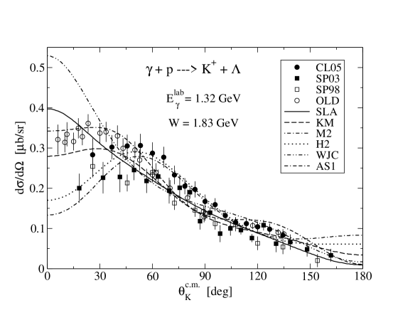
Figure 1: Comparison of various data sets with predictions of different phenomenological models, Saclay-Lyon A (SLA) SLA98 , Kaon-Maid (KM) Ben99 , M2, H2 HYP03 , Williams-Ji-Cotanch (WJC) WJC92 , and Adelseck-Saghai (AS1) AS90 . Data are adopted from Refs. CL05 (CL05), SP03 (SP03), SP98 (SP98), and AS90 (OLD). Total error bars are indicated in the plot.

At present, there are two large data sets, the latest CLAS and SAPHIR ones, with comparable statistical significance, but they diverge in some kinematic regions. Measurements of the differential cross sections at small kaon angles from LEPS LEPS provide another good quality data set for energies from 1.5 to 2.4 GeV. These data are consistent with the CLAS but not the SAPHIR data. The older data, SP98 and OLD, are scarce; and for $\theta_{K}<45^{\circ}$, they also reveal some discrepancies, as shown by open squares SP98 and open circles Bleckmann in Fig. 1. This situation clearly indicates that before a reliable determination of the parameters of a model for the elementary process can be performed, we have to decide which data sets are consistent with each other and which can thus be used in fitting the models. The purpose of this work is to analyze the mutual consistency and similarities of the data sets by using selected isobaric models. The analysis will enable a better determination of the elementary amplitude, especially at forward angles. We also discuss certain problems of the isobaric models with the description of the data at forward directions.

This paper is organized as follows: In Sec. II, the basic formalism and definitions of the kinematic regions used in this analysis are given. The experimental data and the utilized models are briefly discussed in Secs. II A and II B, respectively. In Sec. III, results are presented and discussed. Conclusions are given in Sec. IV.

II Analysis

Although there are some kinematics overlaps of the considered data sets, an interpolation by using an analytical formula is still necessary to perform a direct comparison. To avoid this we compare the observed cross sections with predictions of theoretical models. For this purpose, we calculate the relative deviation for each data point as done in the analysis of OLD data AS90 ,

$$R_{i}=\frac{\sigma_{i}^{\rm exp}-\sigma^{\rm th}(E_{i},\theta_{i})}{\Delta\sigma_{i}^{\rm stat}},$$ (1)

where $\sigma_{i}^{\rm exp}$ and $\Delta\sigma_{i}^{\rm stat}$ are the measured value and its statistical uncertainty, respectively, at the kinematics given by the photon laboratory energy $E_{i}$ and the kaon center of mass angle $\theta_{i}$. The theoretical value $\sigma^{\rm th}(E_{i},\theta_{i})$ is calculated within a particular isobaric model at the appropriate kinematic point. If the theoretical values correctly describe the reality and the experimental values are randomly scattered around them with the variance given by $\Delta\sigma_{i}^{\rm stat}$, then the variable $R_{i}$ possesses a normal distribution with the mean $\mu$=0 and the variance $\sigma^{2}$=1. We are, however, far from this ideal case. The distribution of $R_{i}$, calculated for a particular model and experimental data set, which clearly depends on the chosen model, thus, characterizes a consistency of the model with the data set. To this end, we also calculate the required parameters of the distribution, i.e., the mean value

$$\langle R\rangle=\frac{1}{N}\sum_{i=1}^{N}R_{i},$$ (2)

the second algebraic moment

$$\langle R^{2}\rangle=\frac{1}{N}\sum_{i=1}^{N}R_{i}^{2}=\chi^{2}/N,$$ (3)

the standard deviation

$$s^{2}=\frac{N}{N-1}\langle(\Delta R)^{2}\rangle=\frac{N}{N-1}(\langle R^{2}\rangle-\langle R\rangle^{2}),$$ (4)

and the number of data points with $R_{i}$ in the interval of ($\langle R\rangle-2$, $\langle R\rangle+2$) relative to the number of data $N$, which is denoted by $N_{2}$ (in %). The summations run over the data points included in the sample. The agreement between model predictions and experimental data is expressed by $\chi^{2}/N$ which includes also information on the data dispersion. The mean value $\langle R\rangle$ shows a coherent shift of the data with respect to the model predictions. The condition $\langle R\rangle=0$ is necessary for the model and data to describe simultaneously the reality (a population).

Provided that the data are randomly scattered around the theoretical values $\sigma^{\rm th}(E_{i},\theta_{i})$ with the variance $\Delta\sigma_{i}^{\rm stat}$, i.e. {$R_{i}$, i=1, $N$} is a random sample with a normal distribution, the hypothesis that the true value of the mean $\langle R\rangle$ equals zero (the null hypothesis) can be tested by calculating the statistical parameter (Student’s t-variable) StatMan :

$$z_{1}=\sqrt{N-1}\frac{\langle R\rangle}{\sqrt{\langle(\Delta R)^{2}\rangle}}.$$ (5)

Here, the variance of the normal distribution of $R_{i}$ is supposed to be known and can be approximated by the standard deviation (4), since $N$ is sufficiently large ($>30$) for the assumed data sets. The hypothesis will be rejected with a confidence level of $\alpha$ if $|z_{1}|>z_{\alpha/2}$, where the critical value $z_{\alpha/2}$ = 1.96 and 2.58 for the confidence level of 5% and 1%, respectively StatMan .

In this analysis, we define two types of data samples taken from each of the experimental data sets with different kinematics, i.e.:

• sample A: $0.91$ GeV$<E_{i}<2.6$ GeV and $0^{\circ}<\theta_{i}<180^{\circ}$,

• sample B: $0.91$ GeV$<E_{i}<2.6$ GeV and $0^{\circ}<\theta_{i}<60^{\circ}$.

The statistics of sample B are more sensitive to the differences between the data and model predictions at forward angles, where the largest discrepancies among the data sets and models exist (see Fig. 1). Polarization and total cross section data are not considered in our analysis.

II.1 Experimental data

The following experimental data sets consisting of differential cross sections have been used in calculating $R_{i}$:

• the CLAS data CL05 , labeled by CL05 in the figures and tables,

• the latest SAPHIR data SP03 (SP03),

• the LEPS data LEPS (LEPS), and

• the set of pre-1972 data (OLD), used in the analysis of Adelseck and Saghai AS90 .

Note that the last set is listed in Table IX of Ref. AS90 , except for the data by Decamp et al. (Orsay data). In the CL05 data set, we only consider the data points from threshold up to $E_{\gamma}^{\rm lab}$ = 2.6 GeV ($W=2.4$ GeV, see samples A and B), in order to make an overlap with the SP03 data set and to maintain a reasonable description of the cross sections provided by isobaric models.

The statistical uncertainties of the cross sections were used in the analysis and in the fits of the new models (see the next subsection). The systematic uncertainty of CL05 was estimated to be 8% except for the forward-most angle bins, where the uncertainty amounts to 11% CL05 . For the SP03 SP03 and OLD AS90 data the systematic error bars were reported for each data point. The overall systematic uncertainty of the LEPS data was estimated to be 7% LEPS .

It was shown that the LEPS data are in good agreement with the CLAS data within the total uncertainty and are systematically higher than the SP03 data at all angles ($\theta_{\rm K}^{\rm c.m.}<41^{\circ}$) LEPS . The SP03 data are systematically smaller than the CL05 ones for $W>1.75$ GeV. We note that an energy-independent scale factor of about 3/4 between the CL05 and SP03 results was suggested in Ref. CL05 .

II.2 Models used in the analysis

Theoretical values of the cross sections in Eq. (1) were calculated within the isobaric models for the photoproduction of $K^{+}$ on the proton. In these models the amplitude is constructed by using the Feynman diagrammatic technique, assuming only contributions of the tree-level diagrams. The effective Lagrangian is written in terms of resonant states and asymptotic particles. Because of the absence of a dominant resonance, as in the case of pion and $\eta$ photoproductions, various nucleon and hyperon resonances are considered, which results in a copious number of models Byd03 . Hadrons were supposed to be pointlike particles in the strong vertices in some models SL96 ; WJC92 ; AS90 ; SLA98 but, in the newest ones Ben99 ; HYP03 ; Jan01 , the hadron structure is considered by means of hadronic form factors. The effective coupling constants in the models were determined by fitting the appropriate observables to experimental data.

In our analysis, the Saclay-Lyon (SL) SL96 and Kaon-Maid (KM) Ben99 models were adopted. Common to these models is that, besides the extended Born diagrams, they also include kaon resonances $K^{*}(890)$ and $K_{1}(1270)$. In Ref. WJC92 , it was shown that these $t$-channel resonant terms together with the nucleon ($s$-channel) and hyperon ($u$-channel) resonances can improve the agreement with the experimental data in the intermediate energy region. The models differ in the choice of the particular $s$- and $u$-channel resonances in the intermediate state, in the treatment of the hadron structure, and in the set of experimental data to which the free parameters were adjusted. However, the two main coupling constants, $g_{KN\Lambda}$ and $g_{KN\Sigma}$, fulfill the limits of 20% broken SU(3) symmetry SL96 in both models.

In the SL model, four hyperon and three nucleon resonances with the spin up to 5/2 are included and their coupling constants were fitted to the OLD data set AS90 and the first results of SAPHIR by Bockhorst et al. SAPHIR94 . In the KM model, four nucleon but no hyperon resonances were assumed and the parameters of the model were fitted to the OLD and SP98 SP98 data sets. The SL and KM models were expected to provide reasonable results for photon energies below 2.2 GeV. In our analysis, however, we consider the results of these models for energies up to 2.6 GeV.

In the SL model, hadrons are treated as pointlike objects, in contrast to the KM model in which hadronic form factors (h.f.f.) are inserted in the hadronic vertices Ben99 . The inclusion of h.f.f. in the isobaric model substantially improves the agreement with the higher energy data. However, it appears to be the source of the significant suppression of the cross sections at very small kaon angles and higher energies ($E_{\gamma}>1.7$ GeV, see Fig. 4a in Ref. ProdH and Fig. 1 for M2 and H2 models, which include h.f.f. and were fitted to the results of the first analysis of the CLAS data HYP03 ).

In addition to the KM and SL models, we have also included two new models, which are referred to as fit 1 and fit 2. Fit 1 includes, besides the Born terms and kaon resonances $K^{*}$ and $K_{1}$, the same $s$-channel resonances as in the KM model: $S_{11}(1650),P_{11}(1710),P_{13}(1720)$ and $D_{13}(1895)$. The latter is known as the “missing” resonance, a resonance predicted by the quark model but not yet listed in the Particle Data Book Ben99 . Its presence in the model of this type is, however, important for the description of the resonant structure seen in the SAPHIR and CLAS data Ben99 ; HYP03 . The background part of the amplitude is improved by assuming the $u$-channel resonances as suggested by Janssen et al. Jan01 . Particularly, $S_{01}(1670)$ and $P_{11}(1660)$ hyperon states were chosen in fit 1, as they give the best agreement with the data. The hadron structure in the strong vertices is modeled by the dipole-type form factors introduced by a certain gauge-invariant technique DW01 . The cutoff parameters in the form factors of the Born and resonant contributions are independent. The free parameters of fit 1, i.e. the coupling constants and cutoffs, were determined by fitting the differential cross sections to all CLAS data in the energy region of $E_{\gamma}^{\rm lab}<2.6$ GeV (see the definition of sample A in Section II).

The model fit 1 exhibits a strong suppression of the cross sections at small kaon angles for $E_{\gamma}>1.5$ GeV as discussed above in connection with h.f.f. This pattern, being connected with a strong suppression of the Born terms, particularly the electric part of the proton exchange, causes large deviations of the model predictions from the data at small angles, which precludes analysis of the data at forward angles. To have a more realistic description of the forward-angle data we assume also a model without h.f.f., fit 2. The resonance content of fit 2 was motivated by the SL model, which shows a better agreement with the data in the forward hemisphere than the KM model, especially for energies $E_{\gamma}>1.7$ GeV ($W>2$ GeV, see the next section). Therefore, the following resonances were included in fit 2: the $t$ channel, $K^{*}$ and $K_{1}$; $s$ channel, $P_{13}(1720)$, $D_{15}(1675)$, and $D_{13}(1895)$; and $u$ channel, $S_{01}(1405)$, $S_{01}(1670)$, and $P_{01}(1810)$. The nucleon $P_{11}(1440)$ resonance, which was included in SL but whose coupling constant is very small SL96 , was repalced by $D_{13}(1895)$ to better describe the resonance behavior of the data. The presence of the hyperon $P_{11}(1660)$ resonance, which was also included in the SL model, appears to be irrelevant in the forward-angle region. On the other hand, the higher spin (5/2) s-channel resonance $D_{15}(1675)$ appears to be very important for reduction of the cross section at energy $W>1.8$ GeV and forward angles. Its coupling constants appear to be much larger than those of the other $s$-channel resonances in fit 2. Parameters of fit 2 were fitted to CL05 for energy up to 2.6 GeV but for $\theta_{\rm K}^{\rm c.m.}<90^{\circ}$. Note that the kaon angles were limited in order to avoid problems of these models at backward regions Byd03 (see also the next section) and to achieve a good agreement with the data at forward angles.

In both fits, statistical uncertainties of experimental data (see Sect. II.1) were taken into account and the two main coupling constants were forced to keep the limits of 20% broken SU(3) symmetry: $-4.4\leq g_{KN\Lambda}/\sqrt{4\pi}\leq-3.0$ and $0.8\leq g_{KN\Sigma}/\sqrt{4\pi}\leq 1.3$. The values of the cutoff parameters were also confined in the range of $0.6$ GeV $\leq\Lambda\leq 2.0$ GeV. The best values of $\chi^{2}/{\rm n.d.f.}$ for fit 1 and fit 2 are 3.46 and 1.80, respectively.

III Results and discussion

The statistical parameters of the distributions defined in Section II for samples A and B are listed in Tables 1 and 2, respectively, while the relative deviations of the experimental values from theoretical predictions, $R_{i}$, are displayed in Figs. 2-4. The corresponding mean values, $\langle R\rangle$, are indicated by the dashed lines in each panel of the figures. Panels in a row correspond to the particular model, whereas panels in a column use the same experimental data set (see Section II.1 for the definitions of the data labels and Section II.2 for the definitions of the model labels). In Figs. 2 and 3, the deviations of each data point for all kaon angles (sample A) are plotted as functions of the kaon c.m. angle and the total c.m. energy, respectively. Figure 4 shows results for the forward angles, from $0^{\circ}$ up to $60^{\circ}$ (sample B).

Table 1: Statistical parameters of sample A.

data set	$N$	$\langle R\rangle$	$\chi^{2}/N$	$\langle(\Delta R)^{2}\rangle$	$z_{1}$	$N_{2}$    (%)
model KM
CL05	1109	-0.22	25.7	25.7	-1.41	37.1
SP03	701	-1.04	6.69	5.60	-11.7	68.9
LEPS	60	0.08	45.4	45.4	0.09	26.7
OLD	91	1.00	3.82	2.82	5.66	74.7
model SL
CL05	1109	-17.7	2145	1832	-13.7	1.5
SP03	701	-6.59	198	155	-14.0	7.0
LEPS	60	-0.60	10.1	9.70	-1.47	51.7
OLD	91	-0.09	5.72	5.71	-0.35	68.1
fit 1
CL05	1109	0.15	3.42	3.39	2.66	72.8
SP03	701	-1.24	5.89	4.36	-15.7	70.6
LEPS	60	2.96	31.5	22.7	4.76	20.0
OLD	91	-0.04	11.6	11.6	-0.10	47.3
fit 2
CL05	1109	-6.81	544	498	-10.2	2.5
SP03	701	-3.61	66.8	53.8	-13.0	30.1
LEPS	60	0.26	6.76	6.69	0.77	70.0
OLD	91	-0.32	4.83	4.72	-1.41	59.3

Table 2: Statistical parameters of sample B.

data set	$N$	$\langle R\rangle$	$\chi^{2}/N$	$\langle(\Delta R)^{2}\rangle$	$z_{1}$	$N_{2}$    (%)
model KM
CL05	252	-2.06	37.2	33.0	-5.67	17.1
SP03	178	-1.82	10.0	6.75	-9.30	53.4
LEPS	60	0.08	45.4	45.4	0.09	26.7
OLD	46	1.35	5.43	3.60	4.78	73.9
model SL
CL05	252	-0.05	3.69	3.68	-0.37	70.2
SP03	178	-1.84	8.87	5.48	-10.5	65.2
LEPS	60	-0.60	10.1	9.70	-1.47	51.7
OLD	46	-0.59	4.60	4.25	-1.91	73.9
fit 1
CL05	252	0.22	4.91	4.86	1.60	65.1
SP03	178	-1.00	4.49	3.50	-7.08	75.8
LEPS	60	2.96	31.5	22.7	4.76	20.0
OLD	46	1.12	12.7	11.4	2.23	52.2
fit 2
CL05	252	0.11	1.98	1.97	1.25	84.5
SP03	178	-1.70	7.37	4.47	-10.7	67.4
LEPS	60	0.26	6.76	6.69	0.77	70.0
OLD	46	0.37	3.23	3.09	1.42	78.3

Figure 2: Deviations of the experimental data points from the predictions of the models as a function of cosine of the kaon c.m. angle. The data for the photon laboratory energy below 2.6 GeV are assumed. The mean values of $R$ are represented by dashed lines. Panels in one row correspond to the same theoretical model, whereas panels in the same column use the same experimental data set.

Figure 3: As in Fig. 2, but the deviations are a function of the total c.m. energy. The data cover the full range of the kaon c.m. angle (sample A).

Figure 4: As in Fig. 3, but for experimental data with $0^{\circ}<\theta_{\rm K}^{\rm c.m.}<60^{\circ}$ (sample B).

Table 1 reveals that the $\chi^{2}/N$ values of the model KM are much larger for the CL05 and LEPS data sets than for the SP03 and OLD ones. The SP03 data seem also to be scattered closer to the model predictions than the CL05 and LEPS as indicated by the values of $N_{2}$. However, for sample A the average relative statistical uncertainties, $\Delta\sigma^{\rm stat}/\sigma^{\rm exp}$, are smaller for the CL05 (10%) and LEPS (6%) than for the SP03 (38%) data, which makes the values of $R_{i}$, and therefore $\chi^{2}/N$, much smaller for the SP03. The statistics $|z_{1}|$ in Table 1, which is not sensitive to this effect, shows that the KM model provides a good description of the CLAS ($|z_{1}|=1.41$) and LEPS ($|z_{1}|=0.09)$ data sets (in this case, if we reject the null hypothesis, there is a large probability that we are wrong). On the contrary, the KM model does not seem to be consistent with the SP03, i.e., $|z_{1}|=11.7\gg 2.58$ for the confidence level of 1% (the null hypothesis can be safely rejected).

The very large values of $\chi^{2}/N$ and $|\langle R\rangle|$ for the model SL with CL05 and SP03 data in comparison with those for the KM model are mainly due to the deficiency of the SL model in describing the data at backward angles ($\theta_{\rm K}^{\rm c.m.}>100^{\circ}$) for $W>2$ GeV, as can be clearly seen in Figs. 2 and 3. However, at forward angles, the SL model gives a better agreement with the CL05 and OLD data than the KM model [see the statistics $\langle R\rangle$, $\chi^{2}/N$, $z_{1}$, and $N_{2}$ in Table 2 (sample B) and Fig. 4]. This indicates that the SL model (without h.f.f.) is more suited for the description of the forward-angle data than KM. The SL model also agrees well with the OLD data at backward angles (Table 1), since these data are limited to the photon energies up to 1.5 GeV, and, moreover, they were used to fit the parameters of the model.

The new model, fit 1, which was fitted to the CL05 data for all angle bins (sample A), gives small $\langle R\rangle$ (0.15) but quite large $z_{1}$ (2.66) for CL05 (Table 1), which suggests that the model describes the data with a confidence level smaller than 1%. The largest deviations $R_{i}$ are found, however, for the data at small angles and in the energy range of 1.8 – 2 GeV (see Fig. 4). Comparison of the $\langle R\rangle$ and $\chi^{2}/N$ for fit 1 with CL05 in Tables 1 and 2 also indicates that the model systematically underpredicts the data for small angles. The underprediction of the most-forward-angle cross sections by fit 1 is also apparent for the LEPS data, as obviously shown by Figs. 2 – 4.

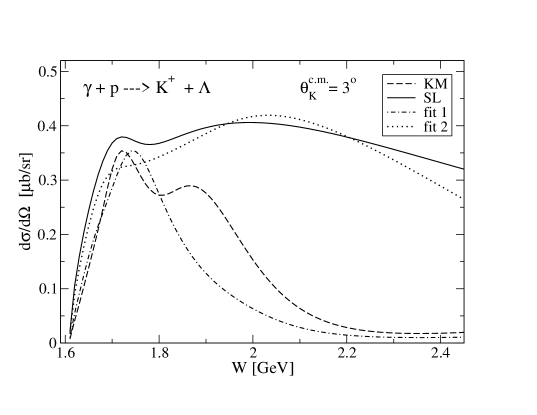
Figure 5: Cross sections at $\theta_{\rm K}^{\rm c.m.}=3^{\circ}$ as predicted by several isobaric models (see text for details).

In Fig. 5 we demonstrate the behavior of the forward-angle ($\theta_{\rm K}^{\rm c.m.}=3^{\circ}$) cross sections as a function of energy for the assumed models. The cross section suppression predicted by the models with h.f.f. (KM and fit 1) is clearly seen for $W>1.8$ GeV. These results suggest that models with h.f.f. introduced in a certain way DW01 cannot provide a realistic description of the forward-angle data. Therefore, the concept of h.f.f. Ben99 ; DW01 should be further investigated to correct the too strong damping of the cross sections at forward angles and larger energies, which is not observed in the existing data.

As expected, the results of fit 2 (fitted only to the forward-hemisphere data) with CL05 at forward angles (sample B) are very good (see Table 2 for the statistics). However, at backward angles, fit 2 reveals the same deficiency as seen with the SL model (see Figs. 2 and 3 and Table 1), although in general fit 2 is much better. The fit 2 model also provides better statistics at forward angles for the LEPS and OLD data than for SP03 (see Table 2), which quantitatively demonstrates that at forward angles the CL05, LEPS, and OLD data can be described simultaneously by an isobaric model without h.f.f. Most of the data are scattered near the model predictions as shown by the large values of $N_{2}$ (defined with the statistical uncertainty) and $|\langle R\rangle|\approx 0$. The values of $|z_{1}|$ are small enough in comparison with the value for the 5% confidence level (1.96), which means that if we reject the null hypothesis, there is greater than 5% probability that we are wrong. On the contrary, the value $|z_{1}|=10.7$ for the SP03 data shows very bad agreement of the SAPHIR data with the model fit 2. Therefore, the hypothesis that fit 2 describes the SP03 data can be ruled out with a very high confidence.

To estimate the relative global scaling factor between the CL05 and SP03 data, we calculated the quantity

$$\chi_{0}^{2}=\sum_{i}\left(\frac{a\;\sigma_{i}^{\rm exp}-\sigma^{\rm th}(E_{i},\theta_{i})}{\Delta\sigma_{i}^{\rm stat}}\right)^{2},$$ (6)

using the SP03 data. The parameter $a$ was chosen to minimize $\chi_{0}^{2}$. For fit 1 and the full data set (sample A), $a=1.13$ and $\chi_{0}^{2}/N=4.80$. These values show that shifting the SP03 data up by 13% improves the agreement with the fit 1 model. For fit 2 and the forward-angle data (sample B), $a=1.15$ and $\chi_{0}^{2}/N=5.29$, which indicates 15% scaling. These results are in good agreement with the estimated systematic uncertainties of the CL05 (8%) and SP03 data. They are, however, smaller than the suggested scaling factor of $\approx 4/3$ CL05 . The coherent shift of the SP03 data with respect to the CL05, LEPS, and OLD ones is also apparent from the comparison of the appropriate values of $\langle R\rangle$ for fit 1 (Table 1) and fit 2 (Table 2). Therefore, this analysis quantitatively shows that a combination of the CL05 and SP03 data should not be considered in fixing the parameters of models, especially at forward angles. Instead, the use of the CL05, LEPS, and OLD data sets is the more preferred choice.

Refitting the fit 2 model parameters using the CL05, LEPS, and OLD data in the forward hemisphere ($\theta_{\rm K}^{\rm c.m.}<90^{\circ}$) yields $\chi^{2}/{\rm n.d.f.}=2.33$ and small changes in coupling constants. The largest changes appear for the coupling constants of the $s$-channel $D_{15}(1675)$ and $u$-channel $P_{01}(1810)$ resonances. We note that the former is important for a proper description of the forward-angle and high-energy cross sections, which is necessary for fitting especially the LEPS data.

Finally, let us discuss the physics consequence of the discrepancy between the CL05 and SP03 data on the fitted resonance parameters. As shown by the recent multipoles approach Mart:2006dk , the use of these data sets individually or simultaneously leads to quite different parameters of resonances which, therefore, could lead to different conclusions about “missing resonances”. Fitting to the SP03 data, e.g., indicates that the $S_{11}(1650)$, $P_{13}(1720)$, $D_{13}(1700)$, $D_{13}(2080)$, $F_{15}(1680)$, and $F_{15}(2000)$ resonances are required, while fitting to the CL05 data leads alternatively to the $P_{13}(1900)$, $D_{13}(2080)$, $D_{15}(1675)$, $F_{15}(1680)$, and $F_{17}(1990)$ resonances. Nevertheless, both CL05 and SP03 support the existence of the missing $D_{13}(2080)$ resonance previously found in the Kaon-Maid model by using the SP98 data SP98 and denoted as $D_{13}(1895)$ (see Section II.2). It was found that the extracted mass of this resonance would be 1936 (1915) MeV if the SP03 (CL05) data were used. We have refitted the original Kaon-Maid model to investigate this phenomenon. The result is shown in Table 3. Obviously, the extracted values corroborate the finding of Ref. Mart:2006dk . The reason that the mass is slightly shifted to a higher value (as well as the broader width $\Gamma$ in the case of CL05) is obvious from the total cross section data (see the second peak of the total cross section shown in Fig. 9 of Ref. Mart:2006dk ).

Table 3: Extracted values of mass $M$ and width $\Gamma$ of the missing $D_{13}$ resonance in Kaon-Maid using three different experimental data sets.

	Original (SP98) SP98	SP03 SP03	CL05 CL05
$M$ (GeV)	$1.895\pm 0.004$	$1.938\pm 0.004$	$1.927\pm 0.003$
$\Gamma$ (GeV)	$0.372\pm 0.029$	$0.233\pm 0.008$	$0.570\pm 0.019$

IV Conclusions

We have analyzed the old (pre-1972) and new (CLAS 2005, SAPHIR 2003, and LEPS) experimental data by comparing them with several existing isobaric models, along with two new models fitted to the CLAS data. Special attention was given to the forward-angles data, i.e. data with $\theta_{K}\leq 60^{\circ}$. The phenomenon of the cross section suppression at forward angles for the isobaric models with the hadronic form factors was observed.

At forward angles, the CLAS 2005, LEPS, and pre-1972 data can be described reasonably well within the isobaric model without hadronic form factors. The SAPHIR 2003 data are systematically shifted below the model predictions which requires a global scaling factor of 15% to remove the discrepancy. The model without hadronic form factors, however, cannot describe the data in the backward hemisphere and at energies $W>2$ GeV.

The isobaric models with hadronic form factors were shown to give too strong damping of the cross sections at small kaon angles and energies $W>1.9$ GeV, which results in a disagreement with existing experimental data. In their present forms, these models are therefore not suited for the description of photoproduction in this kinematic region, which is important, e.g., in the calculation of hypernuclear photoproduction. Needless to say, more precise experimental data at very small kaon c.m. angles ($0^{\circ}-15^{\circ}$) would help solve this problem.

The Saclay-Lyon and Kaon-Maid models do not describe the data satisfactorily as indicated by the statistics $|z_{1}|$ for testing hypotheses. The former model is more consistent with the pre-1972 and LEPS data sets than with the CLAS 2005 and SAPHIR 2003 ones. At forward angles, the Saclay-Lyon model agrees quite well with the CLAS data. The Kaon-Maid model provides a better description of the CLAS 2005, LEPS, and pre-1972 data than the SAPHIR 2003 ones.

The relative-global-scaling factor between the SAPHIR and CLAS data is estimated to be 1.13, which is in agreement with the given systematic uncertainties. This discrepancy was shown to affect the parameters of the “missing” resonance $D_{13}(1895)$ in the Kaon-Maid model. The extracted values of the mass and width of the resonance differ by 11 and 337 MeV, respectively, when the SAPHIR and CLAS data are individually used in fitting the parameters. This finding agrees with the conclusion of a similar analysis that used the multipoles approach Mart:2006dk .

V Acknowledgment

The authors are grateful to O. Dragoun for useful discussions and interest in this work. P.B. acknowledges support provided by the Grant Agency of the Czech Republic, Grant No.202/05/2142 and the Institutional Research Plan AVOZ10480505. T.M. acknowledges the support from the Faculty of Mathematics and Sciences, UI, as well as from the Hibah Pascasarjana grant.

References

- (1) T. Motoba, P. Bydžovský, M. Sotona, K. Itonaga, K. Ogawa, O. Hashimoto, in Proc. Int. Symp. on Electrophotoproduction of Strangeness on Nucleons and Nuclei, Sendai, Japan, 16-18 June, 2003 (World Scientific, Singapore, 2004), p. 221.
- (2) P. Bydžovský, M. Sotona, T. Motoba, K. Itonaga, K. Ogawa, and O. Hashimoto, arXiv:0706.3836.
- (3) T. Miyoshi et al., Phys. Rev. Lett. 90, 232502 (2003); M. Iodice et al., ibid. 99, 052501 (2007).
- (4) R. Bradford et al., Phys. Rev. C 73, 035202 (2006); arXiv:nucl-ex/0509033.
- (5) K.-H. Glander et al., Eur. Phys. J. A 19, 251 (2004); arXiv:nucl-ex/0308025.
- (6) P. Bydžovský and M. Sotona, Nucl. Phys. A 754, 243c (2005); arXiv:nucl-th/0408039.
- (7) J.W.C. McNabb et al., Phys. Rev. C 69, 042201(R) (2004).
- (8) M.Q. Tran et al., Phys. Lett. B 445, 20 (1998).
- (9) A. Bleckmann et al., Z. Phys. 239, 1 (1970).
- (10) T. Mizutani, C. Fayard, G.-H. Lamot, and B. Saghai, Phys. Rev. C 58, 75 (1998).
- (11) T. Mart and C. Bennhold, Phys. Rev. C 61, 012201(R) (1999); T. Mart, ibid. 62, 038201 (2000); C. Bennhold, H. Haberzettl and T. Mart, arXiv:nucl-th/9909022; T. Mart, C. Bennhold, H. Haberzettl, and L. Tiator, http://www.kph.uni-mainz.de/MAID/kaon/kaonmaid.html.
- (12) R.A. Williams, Chueng-Ryong Ji, and S.R. Cotanch, Phys. Rev. C 46, 1617 (1992).
- (13) R.A. Adelseck and B. Saghai, Phys. Rev. C 42, 108 (1990).
- (14) M. Sumihama et al., Phys. Rev. C 73, 035214 (2006).
- (15) E.L. Crow, F.A. Davis, and M.W. Maxfield, Statistics Manual (Dover, New York, 1960).
- (16) P. Bydžovský, F. Cusanno, S. Frullani, F. Garibaldi, M. Iodice, M. Sotona, and G.M. Urciuoli, arXiv:nucl-th/0305039.
- (17) J.C. David, C. Fayard, G.-H. Lamot, and B. Saghai, Phys. Rev. C 53, 2613 (1996).
- (18) S. Janssen, J. Ryckebusch, D. Debruyne, and T. Van Cauteren, Phys. Rev. C 65, 015201 (2001).
- (19) M. Bockhorst et al., Z. Phys. C 63, 37 (1994).
- (20) R.M. Davidson and R. Workman, Phys. Rev. C 63, 025210 (2001).
- (21) T. Mart and A. Sulaksono, Phys. Rev. C 74, 055203 (2006).