Abstract

The influence of the boundary conditions used in the Wigner-Seitz (WS) approximation applied to the neutron star inner crust is examined. The generalized energy functional method which includes the neutron and proton pairing correlations is used. Predictions of two versions of the boundary conditions are compared with each other. The uncertainties in the equilibrium configuration ($Z,R_{c}$) of the crust, where $Z$ is the proton charge and $R_{c}$, the radius of the WS cell, correspond to variation of $Z$ by 2 – 6 units and of $R_{c}$, by 1 – 2 fm. The effect of the boundary conditions is enhanced at increasing density. These uncertainties are smaller than the variation of $Z$ and $R_{c}$ coming from the pairing effects. In the case of high densities, $k_{\mbox{\scriptsize F}}\stackrel{{\scriptstyle\scriptstyle>}}{{\phantom{}{}_{\sim}}}1\;$fm^-1, the most important uncertainty occurs in the value of the neutron gap $\Delta_{n}$. In the WS approximation, it originates from the shell effect in the neutron single-particle spectrum which is rather pronounced in the case of larger $k_{\mbox{\scriptsize F}}$ and, correspondingly, small $R_{c}$ values, but it becomes negligible at lower density near the drip point. An approximate recipe to avoid this uncertainty is suggested.

PACS : 26.60.+c,97.60.Jd,21.65.+f,21.60.-n,21.30.Fe

1 Introduction

In the last two decades the interest on the structure of the neutron star inner crust has been stimulated by the increasing number of observational data on the pulsar glitches. The latter are commonly explained in terms of the dynamics of superfluid vortices within the inner crust of neutron stars (see [1] and Refs. therein). By “inner crust” one usually indicates the part of the shell of a neutron star with sub-nuclear densities $0.001\rho_{0}\stackrel{{\scriptstyle\scriptstyle<}}{{\phantom{}{}_{\sim}}}\rho\stackrel{{\scriptstyle\scriptstyle<}}{{\phantom{}{}_{\sim}}}0.5\rho_{0}$, where $\rho_{0}$ is the normal nuclear density. According to present-day ideas, the bulk of the inner crust consists mainly of spherically symmetrical nuclear-like clusters which form a crystal matrix immersed in a sea of neutrons and virtually uniform sea of electrons. Such a picture was first justified microscopically in the classical paper by Negele and Vautherin [2] within the Wigner-Seitz (WS) approximation. This approximation consists in replacing the crystal by a sum of identical spherical cells with a nuclear cluster at the cell center. As far as the WS method is inconsistent with the crystal symmetry (periodicity), it implies a need for some artificial boundary conditions for the neutron wave functions at the WS cell boundary. To some extent, these conditions are arbitrary provided they guarantee the orthogonality and completeness of the single-particle basis. Unfortunately, calculations with complete taking into account the crystal symmetry are quite complicated. There are only few such calculations, being limited mainly with consideration of the deep (high density) layers of the crust[3, 4], where the “lasagna” or “spaguetti” structure of the crust matter is assumed and the use of the WS method with the spherical symmetry cannot be applied. Only recently a consistent band theory was developed for the outer (low density) layers as well [5]. Therefore up to now the WS method is quite popular and it is usually considered as the most practical one for systematic investigation of the inner crust structure in the whole density interval. For describing the matter of a neutron star crust, Negele and Vautherin used a version of the energy functional method with the density dependent effective mass $m^{*}(\rho)$. In fact, it is very close to the Hartree-Fock method with effective Skyrme forces. For a fixed average nuclear density $\rho$, the nuclear (plus electron) energy functional is minimized for the spherical WS cell of the radius $R_{c}$. A cell contains $Z$ protons (and electrons) and $N{=}A{-}Z$ neutrons ($A=(4\pi/3)R_{c}^{3}\rho$). In addition, the $\beta$-stability condition,

$$\mu_{n}-(\mu_{p}+\mu_{e})=0,$$ (1)

has to be fulfilled, where $\mu_{n}$, $\mu_{p}$ and $\mu_{e}$ are the chemical potentials of neutrons, protons and electrons, respectively. The minimization procedure is carried out for different values of $Z$ and $R_{c}$. The equilibrium configuration ($Z,R_{c}$) at the considered density corresponds to the absolute minimum in energy among all these possible configurations. Application of the variational principle to the energy functional by Negele and Vautherin for a WS cell results in a set of the Shrödinger-type equations for the single particle neutron functions $\phi_{\lambda}({\bf r})=R_{nlj}(r)\Phi_{ljm}({\bf n})$, with the standard notation. The radial functions $R_{nlj}(r)$ obey the boundary condition at the point $r=R_{c}$. As it was noted above, different kinds of boundary conditions could be used. Negele and Vautherin used the following one:

$$R_{nlj}(r=R_{c})=0$$ (2)

for odd $l$, and

$$\left(\frac{dR_{nlj}}{dr}\right)_{r=R_{c}}=0,$$ (3)

for even ones. Let us denote it as BC1. The use of this version of the boundary conditions has been partly justified by physical considerations in [2], but the dependence of the results on the particular choice has never been discussed in detail. It is the purpose of the paper to study this problem at a quantitative level and to establish the corresponding uncertainty, which is inherent to the WS method applied to neutron star crust. For this aim, we compare results obtained for the BC1 with those found for an alternative kind of the boundary conditions (BC2) when Eq. (2) is valid for even $l$ whereas Eq. (3), for odd ones. In principle, two additional kinds of the boundary conditions exist when Eq. (2) or Eq. (3) is used for any $l$. As it was noted in [2], these versions have an obvious drawback for the case of the neutron star inner crust since they lead to an unphysical irregular behavior of the neutron density $\rho_{n}(r)$ in vicinity of the point $r=R_{c}$. Indeed, $\rho_{n}(r)$ vanishes in this point in the first case and has a maximum in the second one. On the contrary, $\rho_{n}(r)$ is almost constant nearby the point $r=R_{c}$ in the case of the BC1 or BC2 kinds of the boundary conditions. It should be noted that the pairing effects were not taken into account in [2] since it was supposed that they are not important for the structure of the crust. The reason of such an assumption is the rather small contribution of the pairing effects to the total binding energy of the system under consideration. Recently, we have generalized the approach by Negele and Vautherin to describe the inner crust by explicitly including the neutron and proton pairing correlations [6, 7, 8, 9] in a self-consistent way. It turned out that in the whole interval of $\rho$ the equilibrium configuration ($Z,R_{c}$) changes significantly due to pairing. To explain this effect, it is instructive to analyze the $\beta$-stability condition (1). Since electrons in the inner crust of a neutron star are ultra-relativistic, the following relation is valid: $\mu_{e}\simeq(9\pi Z/4)^{1/3}/R_{c}$. By substituting it into Eq. (1), one finds

$$Z\simeq\frac{4}{9\pi}(\mu_{n}-\mu_{p})^{3}R_{c}^{3}.$$ (4)

The influence of pairing on the chemical potentials $\mu_{n}$ and $\mu_{p}$ is much stronger than that on the total binding energy. Their variation may be of the order of the gap value $\Delta\simeq$1–2 MeV. Such a variation of $\mu_{n}$ or $\mu_{p}$ may lead to a sizable change of the equilibrium value of $Z$ because the difference ($\mu_{n}-\mu_{p}$) is raised to the third power in Eq. (4). The estimate of the change of $Z$ induced by this variation is as follows: $\delta Z{=}3Z\delta(\mu_{n}-\mu_{p})/(\mu_{n}-\mu_{p})$. For average values of $k_{\mbox{\scriptsize F}}$, the difference $\mu_{n}-\mu_{p}\simeq 50\div 70\;$MeV, hence $\delta Z$ could reach few units of $Z$. An additional change of the $Z$ value may appear due to a variation of $R_{c}$. Besides, as it is shown in [8, 9], the binding energy $E_{B}$ is rather flat function of $Z$ and different local minima $E_{B}(Z)$ have often close values of $E_{B}$. Therefore their relative position may change after switching off the pairing since in general the corresponding contribution to $E_{B}$ is an irregular function of $Z$. Such a situation does often occur within the WS approach, especially for high density values, due to the shell-type effects in the single-particle neutron spectrum. An example is discussed in the paper.

2 Brief description of the method

We used the generalized energy functional method [10] which incorporates the pairing effects into the original Kohn-Sham [11] method. In this approach, the interaction part of the generalized energy functional depends, on equal footing, on the normal densities $\rho_{n},\rho_{p}$, and the abnormal ones, $\nu_{n},\nu_{p}$, as well:

$$E_{\rm int}=\int d{\bf r}{\cal E}_{\rm int}(\rho(\bf r),\nu({\bf r})),$$ (5)

where ${\cal E}_{\rm int}$ is the energy functional density. It is the sum of two components, the normal and the anomalous (superfluid) ones:

$${\cal E}_{\rm int}={\cal E}_{\rm norm}(\rho_{\tau})+{\cal E}_{\rm an}(\rho_{\tau},\nu_{\tau}),$$ (6)

where $\tau=n,p$ is the isotopic index. Just as in the Kohn-Sham method, the prescription $m^{*}=m$ holds to be true. To describe the central part of a WS cell with the nuclear cluster inside we used the phenomenological nuclear energy functional ${\cal E}^{\rm ph}$ by Fayans et al. [10] which describes properties of the terrestrial atomic nuclei with high accuracy. For describing neutron matter surrounding the cluster we used a microscopic energy functional ${\cal E}^{\rm mi}$ for neutron matter based on the Argonne NN potential v₁₈ [12]. The ansatz of [8, 9] for the complete energy functional is a smooth matching of the phenomenological and the microscopic functionals at the cluster surface:

$${\cal E}(\rho_{\tau}({\bf r}),\nu_{\tau}({\bf r}))={\cal E}^{\rm ph}(\rho_{\tau}({\bf r}),\nu_{\tau}({\bf r}))F_{m}(r)+{\cal E}^{\rm mi}(\rho_{\tau}({\bf r}),\nu_{\tau}({\bf r}))(1-F_{m}(r)),$$ (7)

where the matching function $F_{m}(r)$ is a two-parameter Fermi function:

$$F_{m}(r)=(1+\exp((r-R_{m})/d_{m}))^{-1}.$$ (8)

Eq. (7) is applied both to the normal and to the anomalous components of the energy functional. After a detailed analysis, the matching parameters were chosen as follows. The diffuseness parameter was taken to be equal to $d_{m}{=}0.3\;$fm for any value of the average baryon density of the inner crust and for any configuration ($Z,R_{c}$). As to the matching radius $R_{m}$, it should be chosen anew in any new case, in such a way that the equality

$$\rho_{p}(R_{m})=0.1\rho_{p}(0)$$ (9)

holds. In this case, on one hand, for $r<\;R_{m}$ neutrons and protons coexist inside the nuclear-type cluster, and the use of a realistic phenomenological energy functional seems reasonable. On the other hand, at $r>\;R_{m}$ one can neglect the exponentially decaying proton “tails” and consider the system as a pure neutron matter for which an adequate energy functional microscopically calculated can be used. The same matching parameters were used for normal and anomalous parts of (7). As far as practically all the protons are located inside the radius $R_{m}$, the matching procedure concerns, in fact, only neutrons, protons being described with the pure phenomenological nuclear functional. It is worth to mention that for neutron matter region, the ansatz is, in fact, the LDA for the microscopic part of the generalized energy functional. As it is commonly known, the LDA works well only provided the density is smoothly varying, whereas it fails in the surface region with a sharp density gradient. The above choice of the matching procedure and the values of the parameters guarantees that this region of a sharp density variation is mainly governed by the phenomenological nuclear part of the energy functional which “knows how to deal with it”. For the microscopic part of the normal component of the total energy functional (7) we follow to refs. [8, 9] and take the equation of states of neutron matter calculated in [13] with the Argonne v₁₈ potential on the basis of Brueckner theory, taking into account a small admixture of 3-body force. Its explicit form could be found in the cited articles. The microscopic part of the anomalous component of the generalized energy functional in [8, 9] was calculated for the same v₁₈ potential within the Bardeen-Cooper-Schrieffer (BCS) approximation.

3 Comparison of two kinds of boundary conditions, the BC1 versus BC2.

In the calculations of [6, 7, 8, 9] the boundary condition by Negele and Vautherin, BC1, was used. Here we repeat the analysis for the case of the boundary condition BC2. Results for the binding energy per a nucleon, $E_{B}$, are shown in Fig. 1.

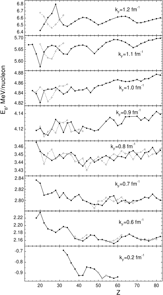
Figure 1: Binding energy per a nucleon for various $k_{\mbox{\scriptsize F}}$ in the BC1 case (solid circles connected with the solid lines) and the BC2 one (open circles connected with the dotted lines).

It is worth to mention that calculations for larger values of $k_{\mbox{\scriptsize F}}$ should be considered as optional as far in this case the spaguetti phase, evidently, is realized. This is true for $k_{\mbox{\scriptsize F}}{=}1.2\;$fm^-1 [14, 3] and, maybe, for $k_{\mbox{\scriptsize F}}{=}1.1\;$fm^-1 [3]. Just as in [8, 9] only even values of Z are used. The detailed comparison is made for $k_{\mbox{\scriptsize F}}{=}0.8\;$fm^-1. Although the two curves $E_{B}(Z)$ are quite different, the positions of local minima for BC1 and BC2 are close to each other, the distance being equal to 2 or 4 units of Z. What is of primary importance, the relative position of local minima for BC2 is the same as for BC1. In particular, the positions of the absolute minimum almost coincide ($Z{=}52$ for BC1 and $Z{=}54$ for BC2). These observations permit us to simplify calculations for other values of $k_{\mbox{\scriptsize F}}$. In the case of BC2, we limit ourselves mainly with the analysis of a vicinity of the absolute minimum for BC1. The neighborhood of other local minima was analyzed only in the case if they have values of $E_{B}(Z)$ close to that corresponding to the absolute minimum. It turned out that there is no value of $k_{\mbox{\scriptsize F}}$ for which the relative position of a local minimum and of the absolute one for BC1 and BC2 is different. In addition to systematic calculations for $k_{\mbox{\scriptsize F}}{=}0.6\div 1.2\;$fm^-1, we made an extra one for a small density, $k_{\mbox{\scriptsize F}}{=}0.2\;$fm^-1, in vicinity of the neutron drip point. In the last case, two curves corresponding to BC1 and BC2 practically coincide. For all other values of $k_{\mbox{\scriptsize F}}$ the absolute minima are shifted by 2, 4 or even 6 units of $Z$. Comparison of different properties of the equilibrium configuration of the WS cell for various values of $k_{\mbox{\scriptsize F}}$ in the case of BC1 and BC2 is presented in Table 1.

Table 1: Comparison of properties of equilibrium configurations of the WS cell for two different kinds of the boundary condition

$k_{\rm F}$,	$Z$	$R_{\rm c},\;$fm		$E_{B},\;$MeV		$\mu_{\rm n},\;$MeV		$\Delta_{\rm F},\;$MeV		$\Delta_{\rm inf}$,
${\rm fm^{-1}}\!$		BC1	BC2	BC1	BC2	BC1	BC2	BC1	BC2	MeV
0.2	52	57.18	57.10	-0.9501	-0.9483	0.1928	0.1942	0.04	0.05	0.40
0.6	58	37.51	37.48	2.1516	2.1596	3.2074	3.2226	1.92	1.89	2.42
	56	36.97	36.95	2.1563	2.1572	3.2173	3.2193	1.91	1.89
0.7	52	32.02	32.04	2.7908	2.7989	3.9876	4.0107	2.30	2.25	2.76
	48	31.16	31.14	2.7924	2.7856	4.0069	3.9873	2.29	2.32
0.8	42	26.90	26.91	3.4373	3.4471	4.8454	4.8561	2.56	2.45	2.93
	44	27.29	27.30	3.4435	3.4319	4.8553	4.8198	2.53	2.56
0.9	24	20.26	20.30	4.1123	4.1169	5.7340	5.7986	2.64	2.51	2.92
	22	19.87	19.70	4.1141	4.1104	5.7861	5.7170	2.62	2.54
1.0	20	16.69	16.90	4.8210	4.8522	6.8525	6.7424	2.02	2.52	2.68
	24	18.29	18.22	4.8479	4.8231	6.8446	6.8920	2.52	2.29
1.1	20	14.99	15.33	5.5765	5.6733	7.4288	8.0446	1.32	2.32	2.26
	26	16.75	17.08	5.6677	5.6100	7.9680	8.5398	2.28	2.02
1.2	20	13.68	13.95	6.4225	6.6762	8.5814	9.1898	1.21	1.56	1.66
	26	15.21	14.89	6.6639	6.4587	9.0825	9.3413	1.25	0.86

There are two lines for every value of $k_{\mbox{\scriptsize F}}$. The first one is given for the $Z$ value corresponding to the minimum of $E_{B}$ in the BC1 case, the second one, for BC2. The only exception is $k_{\mbox{\scriptsize F}}{=}0.2\;$fm^-1 when these two values of $Z$ coincide. In the last couple of columns, the average value $\Delta_{\mbox{\scriptsize F}}$ of the diagonal matrix element of the neutron gap at the Fermi surface is given. The averaging procedure involves 10 levels above $\mu_{n}$ and 10 levels below. For a comparison, the infinite matter value $\Delta_{\rm inf}$ is given in the Table. It is calculated within the BCS approximation for the density of neutron matter corresponding to $k_{\mbox{\scriptsize F}}$ value under consideration. So drastic difference between $\Delta_{\rm inf}$ and $\Delta_{\mbox{\scriptsize F}}$ values in the case of $k_{\mbox{\scriptsize F}}{=}0.2\;$fm^-1 is caused by the trivial reason that this $k_{\mbox{\scriptsize F}}$ is in the vicinity of the neutron drip point. Therefore the asymptotic neutron density which determines mainly the $\Delta_{\mbox{\scriptsize F}}$ value is significantly less than that for the uniform matter distribution. One can see that the influence of the boundary conditions is enhanced at increasing values of $k_{\mbox{\scriptsize F}}$. Especially strong variation of $\Delta_{\mbox{\scriptsize F}}$ and $\mu_{n}$ values takes place in the cases of $k_{\mbox{\scriptsize F}}{=}1.1\;$fm^-1 and $k_{\mbox{\scriptsize F}}{=}1.2\;$fm^-1, see Fig. 2.

Figure 2: The neutron gap for $k_{\mbox{\scriptsize F}}{=}1.1\;$fm^-1, $Z{=}20$ and $Z{=}26$, in the BC1 case (solid lines) and the BC2 one (dashed lines).

To illustrate the influence of the boundary conditions on the neutron gap in the first case, the gap function $\Delta_{n}(r)$ is drawn for both values of $Z$ and both kinds of the boundary conditions. The strongest variation of the gap occurs in the case of $Z{=}20$. To understand the reason of such strong effect, we draw the neutron single particle spectrum $\varepsilon_{\lambda}$ for this value of $Z$ in Fig. 3 for the BC1 case (the left half of the figure) and the BC2 one (the right one). The position of the chemical potential $\mu_{n}$ is shown with dots.

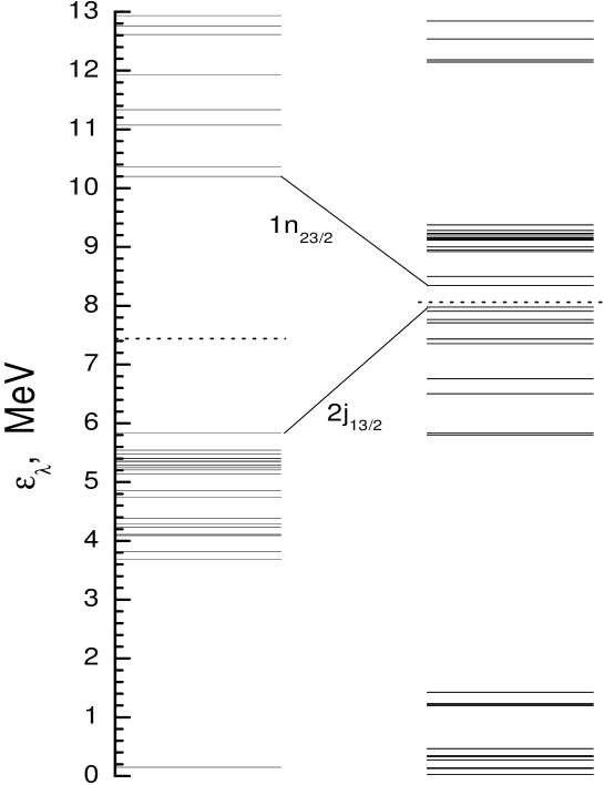
Figure 3: The neutron single-particle spectrum $\varepsilon_{\lambda}$ for $k_{\mbox{\scriptsize F}}{=}1.1\;$fm^-1, $Z{=}20$, in the BC1 case (left) and the BC2 one (right).

The two spectra are absolutely different. The reason is the shift $\Delta\varepsilon_{\lambda}$ of each $\lambda$-level going from BC1 to BC2. The value of this shift is approximately equal to a half of the distance between two neighboring levels with the same ($l,j$), the sign of the shift being opposite for even and odd $l$. The absolute value of the shift is proportional to $1/R_{c}^{2}$ and grows at increasing values of $k_{\mbox{\scriptsize F}}$. The corresponding shifts are shown in Fig. 3 for two states, 2$j_{13/2}$ and 1$n_{23/2}$, which are the neighbors of $\mu_{n}$ in the BC1 case. On average, the spectrum is quite dense, however in both cases there is a shell type structure with rather wide intervals between some neighboring levels. If one deals with a big inter-level space in vicinity of $\mu_{n}$, as in the BC1 case in Fig. 3, one usually obtains a dense set of levels in this region when going to the opposite kind of the boundary conditions. In the BC2 case, big intervals are far from the Fermi surface and do not influence significantly the value of the neutron gap. On the contrary, in the BC1 case $\mu_{n}$ is situated just inside such an interval that suppresses the gap significantly. In principle, the neutron gap could vanish if the interval was wider.

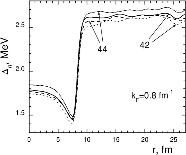
Figure 4: The neutron gap for $k_{\mbox{\scriptsize F}}{=}0.8\;$fm^-1, $Z{=}42$ and $Z{=}44$, in the BC1 case (solid lines) and the BC2 one (dashed lines).

As to the gap function itself, for intermediate densities, $k_{\mbox{\scriptsize F}}<1\;$fm^-1, variations caused by the choice of the boundary conditions are not significant. An example for the case of $k_{\mbox{\scriptsize F}}{=}0.8\;$fm^-1 is given in Fig. 4 where, just as in Fig. 2, four curves for $\Delta(r)$ are shown. The difference between any couple of these curves is less, of course, than the accuracy of the approach. Evidently, the most important uncertainty in the neutron gap value comes from using the BCS approximation without many-body effects like screening, which, for infinite neutron matter, overestimates $\Delta_{n}$ significantly [7].

To be definite, let us consider the “self-consistent” ($Z{=}42$ for $k_{\mbox{\scriptsize F}}{=}0.8\;$fm^-1 ) gap function for the BC1 version of the boundary conditions as the prediction of the WS method for $\Delta(r)$ in the case of small and intermediate densities, $k_{\mbox{\scriptsize F}}<1.0\;$fm^-1. Such a choice corresponds to that used in [9]. The “normal” situation with the gap in the case of intermediate densities corresponds to much more regular single-particle neutron spectra, than that in Fig. 3. For the case of $k_{\mbox{\scriptsize F}}{=}0.8\;$fm^-1 it is illustrated in Fig. 5. One can see that, although here also there are some irregularities in the inter-level distances, they are much smaller than the gap value $\Delta\simeq 2.5\;$MeV. Therefore they don’t influence the gap equation significantly.

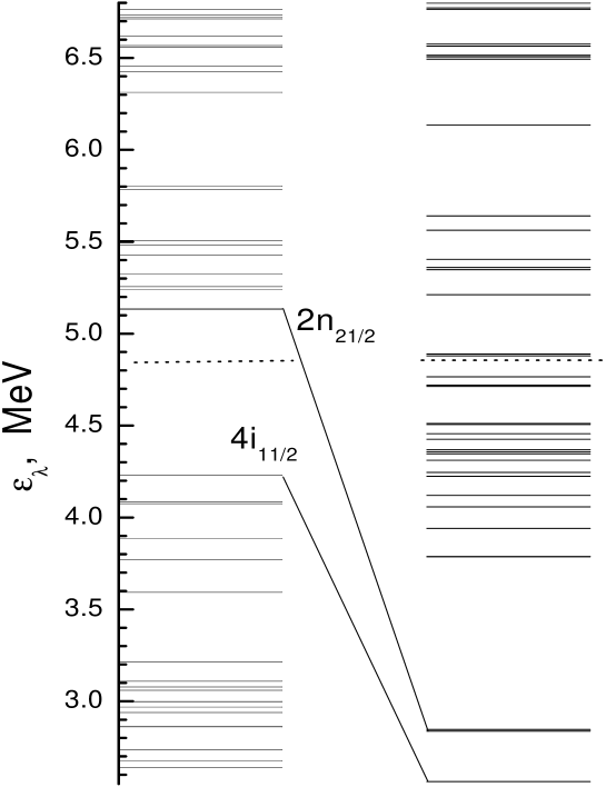
Figure 5: The neutron single-particle spectrum $\varepsilon_{\lambda}$ for $k_{\mbox{\scriptsize F}}{=}0.8\;$fm^-1, $Z{=}42$, in the BC1 case (left) and the BC2 one (right).

In the case of bigger densities, as it is seen in Fig. 2, there is a significant uncertainty in predictions for $\Delta(r)$ within the WS method. As it was discussed above, it originates from the shell-type structure of the neutron single-particle spectrum which appears in the case of high $k_{\mbox{\scriptsize F}}$ (small $R_{c}$) values. We consider this effect as an artifact of the WS approximation which must disappear (or almost disappear) in a more advanced approach with the consistent consideration of the band structure. No doubts, if a forbidden space between two bands in vicinity of $\mu_{n}$ in the band structure calculation will appear, it should be much less than the gap $\Delta$ value. Therefore the solution of the gap equation in the realistic case should be closer to that in the WS approximation for such a situation when there is no big inter-level interval close to $\mu_{n}$. Returning to Fig. 2, these are the dotted line for $Z{=}20$ and the solid one, for $Z{=}26$. Again the difference between these two curves is not essential, and any of them could be used as the prediction for $\Delta(r)$ in the case of $k_{\mbox{\scriptsize F}}{=}1.1\;$fm^-1. Strictly speaking, such a recipe is not a self-consistent one within the WS method, but it looks reasonable from the physical point of view.

4 Discussion and conclusions.

As we have seen, there are internal uncertainties inherent to the WS method applied to the neutron star inner crust which originate from the kind of the boundary condition used. In the case of very small density nearby the neutron drip point the predictions of the BC1 and BC2 versions are practically identical. At increasing density, with $k_{\mbox{\scriptsize F}}\geq 0.6\;$fm^-1, the uncertainty in the equilibrium value of $Z$ is between 2 and 6 units, with the largest values at the largest $k_{\mbox{\scriptsize F}}$. The uncertainty in the value of $R_{c}$ is, as a rule, about 1 fm and only for $k_{\mbox{\scriptsize F}}{=}1.1\;$fm^-1 it turns out to be about 2 fm. However, the value of these uncertainties is smaller than the variations of the equilibrium configuration ($Z,R_{c}$) connected with the pairing effects [9]. For the case of small and intermediate densities , $k_{\mbox{\scriptsize F}}<1\;$fm^-1, the uncertainty in predictions for the gap function $\Delta(r)$ caused by a particular choice of the boundary condition is also rather small. In the case of high densities, $k_{\mbox{\scriptsize F}}\stackrel{{\scriptstyle\scriptstyle>}}{{\phantom{}{}_{\sim}}}1\;$fm^-1, the most important uncertainty occurs in the value of the neutron gap $\Delta_{n}$. In the WS approximation, it originates from the shell effect in the neutron single-particle spectrum which is rather pronounced in the case of big $k_{\mbox{\scriptsize F}}$ and, correspondingly, smaller $R_{c}$ values. We consider this effect as an artifact of the WS method which should disappear in a more consistent band structure calculation. We suggest an approximate recipe to avoid this uncertainty for the gap function $\Delta(r)$. We think that the most important uncertainty in the neutron gap value comes from the BCS approximation used. As it is well known, in neutron matter the many-body corrections to the BCS approximation reduce the value of $\Delta_{n}$ significantly [7]. In the next paper, we plan to take into account this reduction effect for more realistic description of neutron superfluidity in the inner crust of neutron stars.

The authors thank N.E. Zein for valuable discussions. This research was partially supported by the Grant NSh-8756.2006.2 of the Russian Ministry for Science and Education and by the RFBR grant 06-02-17171-a.

References

- [1] C.J. Pethick, D.G. Ravenhall, Ann. Rev. Nucl. Part. Sci. 45 (1995) 429.
- [2] J. Negele, D. Vautherin, Nucl. Phys. A 207 (1973) 298.
- [3] P. Magierski, P.-H. Heenen, Phys. Rev., C 65 (2002) 045804.
- [4] B. Carter, N. Chamel, P. Haensel, Nucl. Phys. A 748 (2005) 675.
- [5] N. Chamel, arXiv preprint: nucl-th/0512034
- [6] M. Baldo, U. Lombardo, E.E. Saperstein, S.V. Tolokonnikov, JETP Lett. 80 (2004) 595.
- [7] M. Baldo, E.E. Saperstein, S.T. Tolokonnikov, Nucl. Phys. A 749 (2005) 42.
- [8] M. Baldo, U. Lombardo, E.E. Saperstein, S.V. Tolokonnikov, Nuc. Phys. A 750 (2005) 409.
- [9] M. Baldo, U. Lombardo, E.E. Saperstein, S.V. Tolokonnikov, Phys. At. Nucl. 68 (2005) 1812.
- [10] S.A. Fayans, S.V. Tolokonnikov, E.L. Trykov, D. Zawischa, Nucl. Phys. A 676 (2000) 49.
- [11] W. Kohn, L.J. Sham, Phys. Rev. A 140 (1965) 1133.
- [12] R.B. Wiringa, V.G.J. Stoks, R. Schiavilla, Phys. Rev. C 51 (1995) 38.
- [13] M. Baldo, C. Maieron, P. Schuck, X. Vinas, Nucl. Phys. A 736 (2004) 241.
- [14] K. Oyamatsu, Nucl. Phys. A 561 (1993) 431.