Relating pseudospin and spin symmetries through charge conjugation and chiral transformations: the case of the relativistic harmonic oscillator
Abstract
We solve the generalized relativistic harmonic oscillator in 1+1 dimensions, i.e., including a linear pseudoscalar potential and quadratic scalar and vector potentials which have equal or opposite signs. We consider positive and negative quadratic potentials and discuss in detail their bound-state solutions for fermions and antifermions. The main features of these bound states are the same as the ones of the generalized three-dimensional relativistic harmonic oscillator bound states. The solutions found for zero pseudoscalar potential are related to the spin and pseudospin symmetry of the Dirac equation in 3+1 dimensions. We show how the charge conjugation and chiral transformations relate the several spectra obtained and find that for massless particles the spin and pseudospin symmetry related problems have the same spectrum, but different spinor solutions. Finally, we establish a relation of the solutions found with single-particle states of nuclei described by relativistic mean-field theories with scalar, vector and isoscalar tensor interactions and discuss the conditions in which one may have both nucleon and antinucleon bound states.
pacs:
21.10.Hw, 21.60.Cs, 03.65.PmI Introduction
Recently, there has been a wide interest in relativistic potentials involving mixtures of vector and scalar potentials with opposite signs. The interest lies on attempts to explain the pseudospin symmetry in nuclear physics. Chen et al. che , using a Dirac Hamiltonian with scalar and vector potentials quadratic in space coordinates, found a harmonic-oscillator-like second order equation which can be solved analytically for , as considered before by Kukulin et al. kuk , and also for . Very recently, Ginocchio solved the triaxial, axial, and spherical harmonic oscillators for the case and applied it to the study of antinucleons embedded in nuclei gin2 . The case is particularly relevant in nuclear physics, since it is usually pointed out as a necessary condition for occurrence of pseudospin symmetry in nuclei gin3 -gin5 . Also the observed isospin dependence of pseudospin can be explained by the effect of the potential on the shape of the potential meng0 -bjp34 . As shown by Bell and Ruegg bell , the and cases correspond to a symmetry of the Dirac Hamiltonian with only scalar and vector potentials which is independent of the particular shapes of these potentials.
A generalized harmonic oscillator (HO) for spin 1/2 particles that includes not only those combinations of scalar and vector potentials, but also a linear tensor potential, giving rise to the so-called Dirac oscillator, has also been considered in nosso . The research of this kind of interaction was started by Itô ito and has been revived by Moshinsky and Szczepaniak mosh1 (see nosso for a complete reference list).
In Ref. nosso a special attention was paid to the case when the scalar and vector potentials are such that , which, as stated before, has been related to the nuclear pseudospin symmetry. There it has been concluded that only when the tensor potential is turned on one gets negative energy bound-state solutions along with the usual positive energy solutions. Those negative energy solutions are important to describe the possible existence of antinucleons in nuclei gin5 . When the tensor potential is absent the special conditions relating the scalar and vector potentials () are needed to have a standard positive HO potential which is only able to bind fermions, and therefore exclude the negative bound-state solutions from the spectra. Actually, as was discussed in another context in asc3 , with an appropriate choice of signs, potentials fulfilling the relations are able to bind either fermions or antifermions. As an example, we will see later that a (negative) harmonic potential, with no tensor potential, binds antifermions and does not allow positive bound-state solutions.
Closely related to this is the fact that, in the nucleus, the charge-conjugation transformation relates the spin symmetry of the negative bound-state solutions (antinucleons) to the pseudospin symmetry of the positive bound-state solutions (nucleons) Zhou . This has also been discussed recently in gin2 , analyzing the HO for antinucleons with spin symmetry () and without the tensor interaction. Again, the charge conjugation connects this problem with the HO for nucleons with pseudospin symmetry (), but in this case the positive harmonic binding potential is . Note that, because the harmonic potential does not vanish for large distances but is a confining potential, it is possible to obtain particle bound-state solutions in the exact pseudospin limit nosso . Therefore, we believe that this connection between spin and pseudospin symmetry obtained by charge conjugation deserves to be more explored. In addition, after the pseudospin symmetry has been revealed as a relativistic symmetry by Ginocchio gin3 , a link of it to chiral symmetry has been suggested based on sum rules calculations in relativistic chiral models that support a small value for furn . However, until now, a clear connection of pseudospin and chiral symmetries has not been established.
The main motivation of this paper is to shed some light in the relation between spin and pseudospin symmetries by means of charge-conjugation and chiral transformations. In order to do so, we solve the mixed scalar-vector-pseudoscalar HO potential in 1+1 dimensions, taking advantage of the simplicity of the lowest dimensionality of the space-time. This approach is equivalent to consider fermions in 3+1 dimensions which are restricted to move in one direction str . We explore the spectra when it is possible to obtain analytical solutions, i.e., in the particular cases when and . As referred before, if the pseudocalar term is turned off, these cases correspond, respectively, to have exact spin and pseudospin symmetry in 3+1 dimensions. We explore all the possible signs of the quadratic ( or ) and linear (pseudoscalar) potentials, thus paying attention to bound states of fermions and antifermions as well. We compare both cases and to establish the charge-conjugation connection discussed above in the presence of the pseudoscalar term. We also consider the case of zero mass to look for the connection between spin and pseudospin symmetries by means of the chiral transformation.
An added motivation for this paper is given by the recent demonstration that the relativistic 3+1 HO with scalar and vector potentials can describe successfully the heavy nucleus spectrum guo . The parameters of the HO are determined by fitting the scalar and vector potentials derived from Relativistic Mean Field nuclear calculations (RMF). The 208Pb neutron single-particle levels obtained in the HO are very similar to the RMF results. The pseudospin symmetry is shown to be almost satisfied for a heavy nucleus in the HO description. The possibility of breaking perturbatively this symmetry in the 3+1 HO by a tensor interaction (in our 1+1 case a pseudoscalar coupling) has been discussed in ronai and can be included in a calculation like the one of Ref. guo in order to improve the results. Thus, the study of all the possible eigenenergies of the 1+1 HO, presented in this paper, considering not only the positive energy solutions already obtained for the 3+1 case in nosso but also the negative ones, can be applied to analyze the existence of antinucleons in nuclei and their spectrum.
The particle and antiparticle spectra we obtain for the cases and demonstrate the charge-conjugation connection referred above. They also show that the spectra of massless states are degenerate with massless states. Further imposing chiral symmetry to these states, such that they would become eigenstates of , would imply that all potentials would be zero and thus one would have just massless free fermions. Our conclusions are valid in the case of 3+1 dimensions, because, as will be shown later, one basically has to add the angular momentum quantum numbers and to the coefficients of the functions appearing in the 1+1 eigenvalue equations in order to get the corresponding 3+1 equations.
This paper is organized as follows. In Sec. II we present the general Dirac equation in 1+1 dimensions with a potential with a completely general Lorentz structure. The effect of charge-conjugation and the chiral transformations upon the general 1+1 Dirac Hamiltonian is discussed in Secs. II.1 and II.2 respectively. In Secs. II.3 and II.4 we present the equations of motion and discuss the isolated solutions, i.e., the solutions out of the Sturm-Liouville problem, for and . The nonrelativistic limits of the and cases are discussed in Sec. II.5, where we show that when there is no nonrelativistic limit when the pseudoscalar potential vanishes or is very small. In Sec. III we introduce the general relativistic harmonic oscillator in 1+1 dimensions for by assigning a quadratic potential for and a linear potential for the pseudoscalar potential . There we also present the eigenvalue equation and the wave functions for bound states, discuss the Dirac oscillator case ( and ) and show how one can use the charge-conjugation and chiral transformations to get the eigenenergies for the case from the case. The following section is devoted to a detailed analysis of the solutions of the relativistic HO for all signs of the parameters and . Finally in Sec. V we discuss the spectrum for and massless fermions and in Sec. VI we draw the conclusions.
II The Dirac equation in 1+1 dimensions
The two-dimensional Dirac equation can be obtained from the four-dimensional one with the mixture of spherically symmetric scalar, vector and anomalous magnetic-like (tensor) interactions. If we limit the fermion motion to the -direction () the four-dimensional Dirac equation decomposes into two equivalent two-dimensional equations with 2-component spinors and 22 matrices str . Then, there results that the scalar and vector interactions preserve their Lorentz structures whereas the anomalous magnetic-like interaction turns out to be a pseudoscalar interaction. Furthermore, in the 1+1 world there is no angular momentum so that the spin is absent. Therefore, the 1+1 dimensional Dirac equation allows us to explore the physical consequences of the negative-energy states in a mathematically simpler and more physically transparent way. In this spirit the two-dimensional version of the anomalous magnetic-like interaction linear in the space coordinate has also received attention nogami -asc1 . Later this system was shown to be a particular case of a more general class of exactly solvable problems asc2 .
Let us begin by presenting the Dirac equation in 1+1 dimensions. The Dirac equation for a particle with mass and a general potential , to be defined later, is formally the same as its 3+1 counterpart:
| (1) |
Here and the matrices obey the usual relations , where is the identity matrix. The metric tensor and the covariant derivative operator are, respectively, and . The Hamiltonian is defined in the usual way, such that Eq. (1) is written as
| (2) |
where . The positive definite function , satisfying a continuity equation, is interpreted as a position probability density and its norm is a constant of motion. This interpretation is completely satisfactory for single-particle states tha . The traceless matrices and are defined by and , and obey the relations , . We set to be
| (3) |
where . This is the most general combination of Lorentz structures because there are only four linearly independent 22 matrices. The subscripts for the terms of the potential denote their properties under a Lorentz transformation: and for the time and space components of the 2-vector potential, and for the scalar and pseudoscalar terms, respectively.
If the terms in the potential are time-independent, the Dirac equation (2) becomes
| (4) |
where
| (5) | |||||
| (6) |
and is the fermion energy. To have an explicit expression for the and matrices one can choose 22 Pauli matrices which satisfy the same algebra. We use , and thus .
The Hamiltonian (5) is invariant under the parity operation, i.e., when , and change sign, whereas and remain the same. This is because the parity operator is , where is a constant phase and changes into . Since this unitary operator anticommutes with and , they change sign under a parity transformation, whereas and , which commute with , remain the same. When one writes down the explicit equations of motion in terms of the components of the spinor , the combinations and of the vector and scalar components arise naturally. Therefore, it is convenient to rewrite the Hamiltonian (5) in terms of these potentials. We have
| (7) |
II.1 Charge conjugation
The charge-conjugation operation changes the sign of the electromagnetic interaction, i.e., changes the sign of the time and space potentials in (3). This is accomplished by the transformation (see, for example, Itzykson and Zuber Itzykson_Zuber )
| (8) |
where denotes matrix transposition and is a matrix such that . In dimensions one matrix that satisfies this relation is
If we choose the phase factor equal to 1, we have
| (9) |
After applying this charge-conjugation operation to the Dirac equation (2), the time-independent Dirac equation becomes
| (10) |
where and is given by
| (11) |
In terms of the potentials and , this Hamiltonian reads
| (12) |
One sees that the charge-conjugation operation changes the sign of the energy and of the potentials , and . In turn, this means that turns into and into . Therefore, to be invariant under charge conjugation, the Hamiltonian must contain only a scalar potential.
II.2 Chiral transformation
The chiral operator for a Dirac spinor is the matrix , and we will call “chiral transformation” the transformation associated with it. Thus, the transformed spinor is given by and the transformed Hamiltonian . Since anticommutes with , the time-independent chiral-transformed Dirac equation is
| (13) |
where is given by
| (14) |
or
| (15) |
in terms of and . This means that the chiral transformation changes the sign of the mass and of the scalar and pseudoscalar potentials, thus turning into and vice-versa. A chiral-invariant Hamiltonian needs to have zero mass and and zero everywhere.
II.3 Equations of motion
The space component of the 2-vector potential in (3) can be absorbed into the wave function by defining a new spinor such that
| (16) |
in which , since we have . From this point on, we will refer to as simply a vector potential, following the common usage of this term (usually denoted by ). If we now write the spinor in terms of its components,
| (17) |
the Dirac equation gives rise to two coupled first-order equations for and :
| (18) | |||||
| (19) |
where the prime denotes differentiation with respect to . In terms of and the spinor is normalized as , so that and are square integrable functions. It is clear from the pair of coupled first-order differential equations (18) and (19) that and have opposite parities if the Dirac equation is covariant under .
Under the charge-conjugation and chiral transformations the spinor (17) becomes
| (20) |
and
| (21) |
respectively.
II.4 The Sturm-Liouville problem and isolated solutions
Using the expression for obtained from (19) with , viz.
| (22) |
and inserting it in (18) one arrives at the following second-order differential equation for :
| (23) |
In a similar way, using the expression for obtained from (18) with , viz.
| (24) |
and inserting it in (19) one arrives at the following second-order differential equation for :
| (25) |
For with , (22) and (23) reduce to
| (26) |
| (27) |
and for with , (24) and (25) reduce to
| (28) |
| (29) |
Either for with or with the solution of the relativistic problem is mapped into a Sturm-Liouville problem in such a way that solution can be found by solving a Schrödinger-like problem. If one considers potentials and quadratic in with and a potential linear in one obtains Schr’́odinger-like equations for the harmonic oscillator potential.
The solutions for with and with , excluded from the Sturm-Liouville problem, can be obtained directly from the original first-order equations (18) and (19). They are
| (30) |
and
| (31) |
where and are normalization constants. Since, by parity conservation, must be an odd function of , its integral must be an even function of . Thus, if the integral of has a definite sign, its overall sign can determine whether the isolated solutions (30) and (31) are bound states. In particular, if and or are powers of , one sees from each pair of equations (30) and (31) that, in general, one of the spinor components has to be zero, either in the first case (sign of the coefficient positive) or in the last case (sign of the coefficient negative). This is the case of the harmonic oscillator potentials, as we will see in the next section. However, it is possible find solutions with the coefficient negative in the first case (, ) and with the coefficient positive in the second case (, ), provided a certain relation between the coefficients of all the potentials is satisfied, as we will see later.
II.5 The nonrelativistic limit
In the nonrelativistic limit, , Eq. (23) becomes
| (32) |
where . Since, in the nonrelativistic regime, for the range of values of in which the wave function is not negligible, , from Eq. (22) we see that is of order relative to , provided, of course, one has also . On the other hand, since in these conditions and the term in Eq. (32) is suppressed relative to the other terms, we also see that obeys a Schrödinger equation with binding energy equal to .
We shall consider now the nonrelativistic limit in the special cases and , which we will also consider later in the paper when we solve the Dirac equation for harmonic oscillator potentials.
When , Eq. (32) becomes
| (33) |
Here we clearly see that plays the role of a binding potential in the nonrelativistic limit and that gives rise to effective binding potentials proportional to and . This means that even a pseudoscalar potential unbounded from below could be a confining potential. Note that if is of the same order that in a expansion within the classically accessible region (positive kinetic energy) where the wave function is not negligible, and if its variation over this region is such that ( changes very little over a distance of the order of a Compton wavelength), gets suppressed relative to .
For the case and if is very small in the classically accessible region, Eq. (32) becomes
| (34) |
If or if, as explained before, the and terms are higher-order terms in a expansion within the classically accessible region, Eq. (34) becomes a free particle Schrödinger equation. This is in agreement with what was found in Ref. nosso , namely that when and is a three-dimensional harmonic oscillator potential, there is no nonrelativistic limit. In this case we were able to show that this is true in a more general framework. A model for a relativistic particle in which the vector and scalar potentials are such that , and where the pseudoscalar potential is suppressed, is intrinsically relativistic, as far as bound states are concerned.
This last result deserves some more comments. The fact that in a Dirac equation one can have Lorentz scalar and pseudoscalar potentials leads to remarkable results that are at odds with what is known from nonrelativistic quantum mechanics, where the Lorentz structure plays no role, since one has only potentials which couple to the energy, i.e., behave as time components of a relativistic vector. Among these results is the fact that the Dirac equation is not invariant under a simultaneous shift of the energy, the scalar potential, and the pseudoscalar potential. It has already been verified that a constant added to the pseudoscalar screened Coulomb potential asc10 or to the pseudoscalar inversely linear potential asc100 is physically relevant and plays a crucial role in ensuring the existence of bound states. As an example of another notable result, it is well known that a confining potential for a nonrelativistic fermion cannot confine it in the relativistic regime when the potential is considered as a Lorentz vector (see, e.g., tha ), simply because there is pair creation and the single-particle picture does not hold anymore. It is surprising that the converse is also true, i.e., that relativistic binding potentials may not bind in the nonrelativistic limit. This is the case of () referred before, and is basically due to the fact that vector potentials couple in a different way than scalar potentials in the Dirac equation, whereas there is no such distinction in the Schrödinger equation. Actually, as we have seen before, , which is the sum of a vector and a scalar potential, plays the role of a binding potential in the nonrelativistic limit, whereas a weak enough cannot bind a fermion with nonrelativistic energy if . Note that for potentials going to zero at infinity, like mean-field nuclear potentials, there are no bound states when , even if is not small compared with fermion rest energy gin3 -alb2 .
Regarding antiparticles, an attractive vector potential for a particle is, of course, repulsive for its corresponding antiparticle, and vice versa. However, the attractive (repulsive) scalar potential for particles is also attractive (repulsive) for antiparticles. This is expressed in the change and under charge conjugation, as referred in Sec. II.1. This means that an antiparticle with nonrelativistic energies () will not be bound when , provided is small enough.
III The relativistic harmonic oscillator
Let us consider
| (35) |
As we have seen in the last section, the chiral transformation performs the changes , , and . Morever, since interchanges the upper and lower components (see (21)), the resulting pair of transformed equations of motion are formally the same, so that their solutions have the same energy eigenvalues. This symmetry can be clearly seen from the two equation pairs (22)-(23) and (24)-(25) as well as from the isolated solutions (30) and (31) which are converted into each other by this kind of transformation. This means that one can restrict the discussion to the case (). The results for the case when can be obtained immediately by just changing the sign of and of in the relevant expressions.
The Dirac spinor corresponding to the isolated solution with is obtained from (30). Only for there is a normalizable Dirac spinor and, as commented before, the upper component vanishes whereas the lower component is given by , regardless the value of . For , Eq. (27) takes the form
| (36) |
where
| (37) | |||||
| (38) |
The well-behaved solution for (36), with necessarily real and positive, is the well-known solution of the Schrödinger equation for the nonrelativistic harmonic oscillator (see, e.g., sch ):
| (39) | |||||
| (40) |
where , is a normalization constant, is a -th degree Hermite polynomial and
| (41) |
The lower component of the Dirac spinor is obtained from (26). When one uses the recursion relations for the Hermite polynomials (see, e.g., abra ) one gets
| (42) |
Since the Hermite polynomial has distinct zeros one may conclude that has nodes, and the expression for suggests that it has nodes, depending on the sign . In fact, if , this last expression reduces to
| (43) |
showing that is proportional to if is positive. If , the recursion relations of Hermite polynomials imply that is proportional to (see abra ).
From Eqs. (37), (38) and (40) we can get the quantization condition for the Dirac eigenenergies:
| (44) |
The nonrelativistic limit is reached when and . In this case for small quantum numbers, and Eq. (44) becomes
| (45) |
so that is restricted to .
In general there is no requirements on the signs of and , except that, as stated before, , and therefore, from (37), the Dirac eigenenergies corresponding to the bound-state solutions must be within the limits
| (46) | |||||
| (47) |
For , when there is a pure pseudoscalar potential linear in (the two-dimensional Dirac oscillator), Eq. (44) reduces to
| (48) |
Note that for and for , because for the latter case the lower component is proportional to a Hermite polynomial of degree . This result, together with Eq. (48), allows us to conclude that the Dirac eigenvalues are given by , where , , irrespective of the sign of . This means that the spectrum is independent of the sign of . The solutions and correspond to isolated solutions for and , respectively (see Eqs. (30) and (31)). However, the spinors do depend on the sign of , because different signs induce different node structures, as can be seen from (43). Since the charge-conjugation transformation changes the sign of , it connects both kinds of solutions, but each can have both positive and negative energies. Thus a complete set of states for a certain includes both particle (positive energy) and antiparticle (negative energy) states but they are not related to each other by a charge-conjugation transformation. The spectral gap between these solutions is and does not disappear when . Therefore, there is no room for transitions from positive- to negative-energy solutions and Klein’s paradox never comes into play. There are no scattering states when , but for the continuum states are those ones which have energies beyond the limits expressed by (46)-(47), for which . As far as the chiral transformation is concerned, one can note that acts much in the same way as the charge-conjugation transformation, except that it does not change the sign of the energy and changes the mass sign. Therefore, the chiral transformation connects solutions with the same energy sign but that have opposite signs.
When , i.e., no pseudoscalar potential, there is no isolated bounded solutions and the quantization condition expressed by Eq. (44) takes the form
| (49) |
where stands for the sign function. This means that when there are only bound states for fermions with and those bounded solutions are kept apart from the negative-energy continuum () by an energy gap greater than . On the other hand, for there are only bound states for antifermions with and those bounded solutions also do not mix with continuum states with . Therefore, the positive-energy bound states of fermions never sink into the Dirac sea of negative energies, and the negative-energy bound states of antifermions never reach the upper continuum, so again there is no danger of reaching the conditions for Klein’s paradox. It is important to note that the solutions with are not the antiparticles of the solutions with because charge conjugation changes into and vice-versa. This means that the antiparticles of the states with and are the negative-energy solutions of the relativistic system with , with positive.
To conclude, let us present, as an example of the rule stated at the beginning of the section, the eigenvalue equation for the relativistic harmonic oscillator when :
| (50) |
Here is the number of nodes (the degree of the Hermite polynomial) for the lower component, since the chiral transformation interchanges the upper and lower components, so that the second-order equation to solve in this case is the one for the lower component, Eq. (29). The upper component would be obtained from the corresponding first-order equation Eq. (28). As a final remark, one may note that for massless particles, the and oscillators have the same spectrum with the sign of reversed.
In 3+1 dimensions the corresponding eigenvalue equations to Eqs. (44) and (50) have a very similar structure. From nosso we see that, for , one just adds the Dirac equation quantum number to the coefficient of and modifies the coefficient of the square root to include the orbital angular momentum of the upper component
| (51) |
while for one uses the orbital angular momentum of the lower component
| (52) |
where (see nosso ). If we compare these equations with (44) and (50), we see that the main features are identical, and thus all the main results obtained in the next section remain valid for the relativistic harmonic oscillator in three spatial dimensions.
IV Graphical determination of the energy levels
We turn now to the solutions of Eq. (44). In order to obtain a deeper insight on those solutions for arbitrary and one has to seek a convenient method for solving this transcendental equation. If we square Eq. (44) the resulting equation is in general a quartic algebraic equation in , which in principle can be solved analytically. The price paid is that some spurious roots can appear in this process, although, of course, these can be eliminated by checking whether they satisfy the original equation. A more instructive procedure is follow a graphical method, by which one seeks the intersection points of the functions of energy in Eq. (44): a parabola on the left-hand side
| (53) |
and a square-root function on the right-hand side
| (54) |
In this way, it is easy to see that there are at most two acceptable solutions of (44), since the parabola and the square-root function can have at most two intersection points. The construction of the graph of is split into three distinct classes depending on the values. Below we discuss these three classes of problems. It should not be forgotten, though, that the solutions with are not included in this discussion, since they correspond to isolated solutions for .
This kind of analysis and the conclusions that will be drawn from it in the following subsections can be applied with appropriate modifications to the 3+1 case, and therefore to nucleon and antinucleon single-particle spectra. This is especially true as far the relations between the spectra of systems with and are concerned, since these are obtained from the general properties of charge-conjugation and transformations which hold in 3+1 dimensions.
IV.1 The case
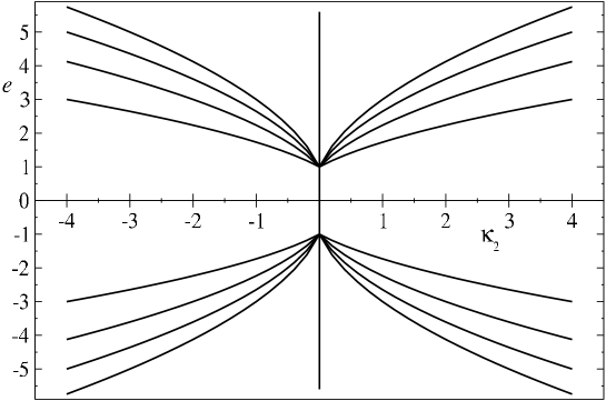
Although we have already solved this case, it is presented here for the sake of completeness. For , is just a nonnegative constant function as can be seen from Eq. (48), having two symmetric intersections with the parabola.
Fig. 1 and Fig. 2 present the results for the first four quantum numbers. In these and the following plots we use the scaled quantities , and . The first shows how the values of the energy are obtained from the intersection of the two curves and the second how the eigenvalues vary with . The energies for the zero mass case can also be computed from the intersections with the dashed parabola in Fig. 1. From these figures it is clear the symmetry of the energy levels. Note again that the isolated solution is not plotted.

IV.2 The case
When , is a monotonically increasing function of . For each , it can intersect the parabola at one or two points, depending on the particular values of and . To determine the conditions for this to occur, we have first to determine the minimum of , which occurs when the expression under the square root in (54) is zero:
| (55) |
This value sets a lower bound for the energies of all the solutions of Eq. (44). For , the function takes the value
| (56) |
and takes the value
| (57) |
When , the minimum of occurs for negative values of the energy, that is, on the left (and decreasing) side of the parabola. If there is only one solution of Eq. (44) and it has positive energy. From (56), this can happen only for , since . If there are always two solutions, one negative and one positive, because is always positive, no matter how large is , for a positive . Furthermore, the positive and negative solutions are such that , since, when , and thus there are no solutions. Note, however, that for and negative there is a solution with , but this is an isolated solution out of the Sturm-Liouville problem we are considering.
The considerations of the previous paragraph can be further elaborated by analyzing the behavior of the function
| (58) |
According to what was stated in the previous paragraph, if one has two solutions for each , and if there is just one solution for each . To determine the signs of for each value of , we will need to know the values of which are roots of , or of the equation
| (59) |
excluding the solution . Applying Descartes’ rule of signs to this last equation, we see that it can only have a positive real solution. The rule states that the number of positive real roots of an algebraic equation with real coefficients
| (60) |
is never greater than the number of changes of signs in the sequence (not counting the null coefficients) and, if less, then differs from by an even number. This means that can take the values , . In this case, for positive , there is only one such sign change and therefore there is only a positive and unique solution, which we shall call . The function changes sign at and , being negative in the interval and positive outside this interval. Therefore, according to what we have said before, there is only one positive-energy solution when and two solutions (one positive and one negative) when or . If , the two functions intersect at , but again, since this solution was excluded from the Sturm-Liouville problem leading to the eigenvalue equation (44), we consider only the harmonic oscillator solutions with energy greater than .
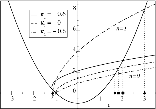
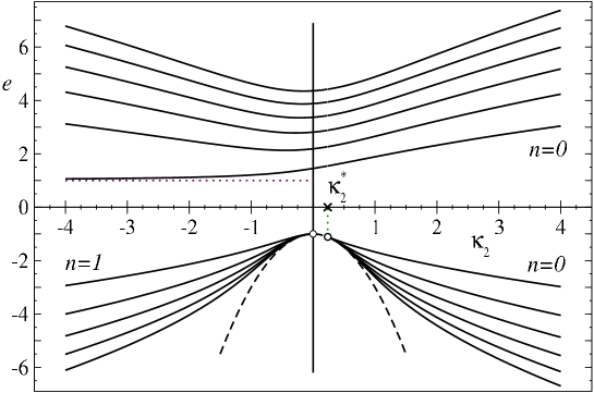
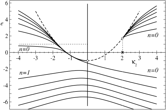
The graphical representations of and are shown in Fig. 3 for . We plot the square-root function for three values of (the scaled ), for a positive . We plot with for and with and for . The value of was chosen such that has a positive value for . There is always an infinite and unbounded set of positive-energy states with for any value of , and there are always negative states when is negative. Note that increasing the value of does not change qualitatively these features, as can be seen from the plots of when is negative.
In Fig. 4 it is clearly seen that for values of between zero and there are only positive-energy solutions. Moreover, one can see from Eq. (59) that the value of increases with , meaning that when one reaches the limit of the harmonic oscillator () where there are only positive bound-state solutions with . Thus, the existence of the pseudoscalar potential gives rise to negative-energy solutions coming from the Dirac sea. For these kind of solutions always exist. We excluded the isolated level with for negative . Note also that for decreasing negative the positive-energy solution for goes to , which was the case we discarded in the discussion of the Dirac oscillator in the previous section. When there is an infinite set of degenerate solutions with , because in this case the intersection point of with the negative-energy branch of is the initial (minimum) point of the square-root function, which of course does not change with (see Fig. 3). However, when , the value of defined in (37) is zero, and thus, from (41), and therefore these solutions do not correspond to bound states (see Eqs. (39) and (42)). For the degeneracy is removed and we have a very high density of very delocalized states (since ) which then decreases with increasing . In Fig. 4 we also plotted the parabola (in scaled units ) which corresponds to the asymptotic values of the negative-energy states when and thus represents the set of lower energy bounds of the negative-energy solutions for each pair of and values. This parabola can be also seen as delimiting the region in the energy- plane in which , i.e., where there are no bound-state solutions. This is related to the discussion in the previous section leading to Eqs. (46) and (47).
As referred before, for a given energy and positive there are not bound states for values of in the interval . In fact, from what was said above in this section, one can be more precise and state that there are no negative bound states for . Since is zero when and increases with increasing , this means that when (the Dirac oscillator) there are no continuum states and when (or when ), all the negative-energy states are continuum states.
IV.3 The case
For the function decreases monotonically with the energy, reaching again its minimum when the expression under the square root in (54) is zero, setting now a maximum value for the energy of the solutions of Eq. (44). The expressions for , and are the same as corresponding ones in the previous subsection, respectively Eqs. (55), (56) and (57), except that, of course, now is negative.
Noting that at has a nonnegative value given by , we see that there is always an infinite and unbounded set of negative-energy solutions (one for each ) with . For and , there is a solution with which was already discussed in the previous section. However, when , one can solve Eq. (30) when and obtain a bound-state solution with both upper and lower components different from zero, if and only if . One can show that this corresponds to a solution given by the functions (39) and (42) taking the limit .
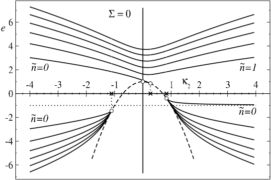
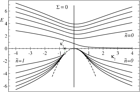
In addition to that set of solutions, there can be another set of solutions only if the function (see Eq. 58) is zero or positive, as explained before. To determine the values of for which this happens, one has to compute the roots of . When , Descartes’ rule of signs applied to states that one can have a positive root and two or zero negative roots (this is done by changing in (60)), in addition to, of course, the root . The two negative roots arise for a value of such that . In scaled units, this value is , corresponding to the double negative root . For there is only a positive root, while for there are two negative roots and a positive root. Because changes sign at (except when is a double root) and is always positive when , this means that when there is only one range of values of where whereas when there are two ranges of values where this happens. Within these ranges, only negative-energy solutions exist. When , the value corresponds to an infinite set of degenerate negative-energy solutions with scaled energy , which, as mentioned before, are not bound-state solutions. These features of the spectrum can be seen in Figs. 5 and 6.
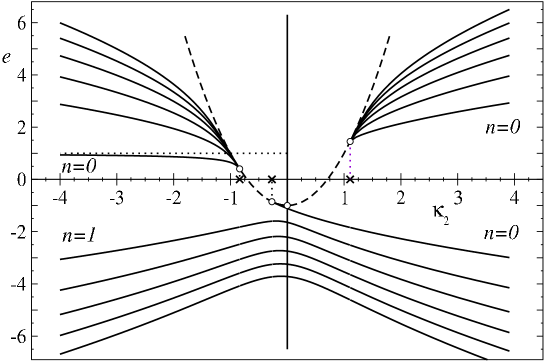
In Fig. 5 the solutions with with are basically degenerate (they follow closely the parabola ) and the solution is very close to them. Since, as remarked before, on the parabola the value of is zero, these are very weakly bounded solutions. Note that the positive-energy solution with goes to when , thus becoming the isolated solution of the Dirac oscillator (). This can also be seen in Fig. 6, where one may also remark that there is a value of around for which the solutions for distinct values of and are almost degenerate. This point corresponds to the local minimum of , which, for , is very close to the double root . Similarly as in the case of , the solutions with have infinite degeneracy, but they do not correspond to bounded solutions. Again, for near there is a high density of very delocalized states. The parabola sets now an upper bound () for the positive-energy states.
The limits and correspond, respectively, to the harmonic oscillator solutions for negative-energy (antiparticle) states and to the Dirac oscillator. In the first case there are no bound states for particles (positive-energy states). As increases, positive bound states start to appear.
IV.4 Variation with for fixed
To complete the study of solutions of equation (44) we present now a plot of its solutions when is kept fixed and let vary. Note that the existence of one or two solutions is governed by the sign of the function
| (61) |
identical with , except that now acts as a parameter and is the variable. The critical value is now . In Fig. 7 we present a plot of the solutions for , when there are two possible values for , the roots of . Apart the factor , this is just a quadratic equation in , so that it is easily shown that when it has no real solutions. This means that, since in this case , there are always two sets of solutions. Note that now the points in the energy- plane for which are on the hyperbole , such that only in the region between the hyperbole branches, where is positive, bound states may exist.
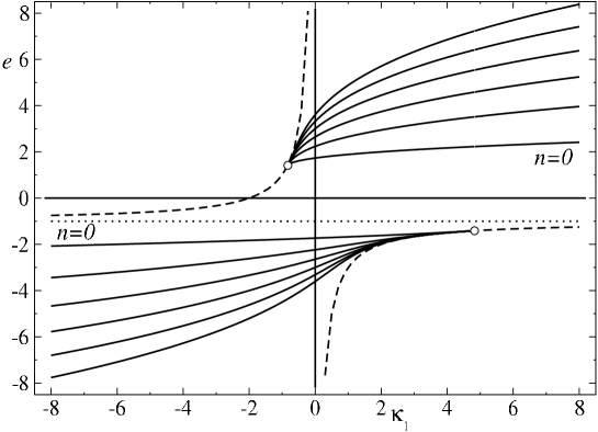
As before, we can recognize the Dirac oscillator and the harmonic oscillator limits, as one sets and , respectively. In this last case, one has the harmonic oscillator solutions for particles or antiparticles depending whether goes to or . One can again see that the energy levels of the Dirac oscillator are symmetric about and that there are no scattering states. Here this follows simply from the fact that is an asymptote of the hyperbole branches which separate the continuum region from the bound-state region.
V Solutions from symmetry arguments
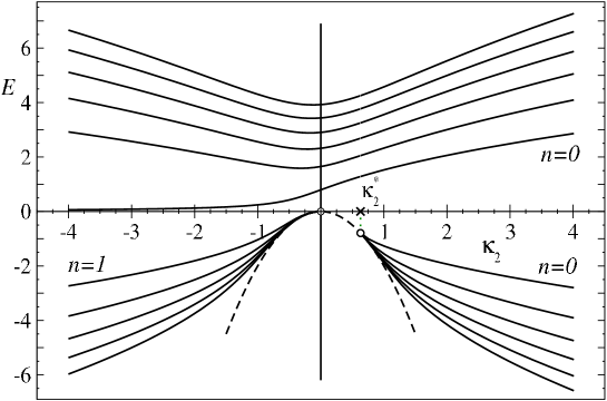
As referred before, the case can be obtained from the case by applying the charge-conjugation transformation. We recall that this transformation performs the changes , and , or, for harmonic oscillator potentials, the changes and . This can be seen if we solve the eigenvalue equation for , Eq. (50), for and plot the solutions for several values of . The result is shown in Fig. 8.
If we compare this figure with Fig. 5 () we see that the plots are identical if we reverse both the vertical and horizontal axes, i.e, if we reverse the sign of the energy and of , respectively. Of course, the identification of the particle and antiparticle levels is also reversed, as it should be, since we are applying the charge-conjugation transformation.
The existence of both positive- and negative-energy solutions in a system with can be relevant for nuclei. In the 3+1 Dirac equation of relativistic nuclear mean-field theories there is a connection between the (isoscalar) vector and tensor potential. The latter is proportional to the derivative of the former nosso2 . For the harmonic oscillator potentials used in this paper, this would give, using the notation of Ref. nosso2 , the relation
| (62) |
The constant can take values up to around 1.3 in nuclei using relativistic mean-field potentials of Woods-Saxon type nosso2 . For harmonic oscillator mean-field potentials, there should be also an upper value for , and therefore the relation (62) sets a maximum for in nuclei. As was seen above, this is relevant to know whether there can be simultaneously nucleon and antinucleon bound states in nuclei. This would depend very much on the strength of the potential, which is given by . As is apparent from Fig. 8, for small values of the scaled , , the maximum value of allowed by Eq. (62) could be such that there would exist only positive-energy states. On the other hand, for stronger potentials, the relation (62) could allow both positive- and negative-energy bound states, as can be seen by applying the axis reversal described above to the spectrum shown in Fig. 6.
In Sec. III we have seen that the chiral transformation can also be used to get formally from solutions, involving, however, the unphysical transformation . This objection is overcome when we deal with ultrarelativistic particles, for which we may consider . In this case, the chiral transformation relates massless physical states with and a pseudoscalar potential to massless states with and , where can be an arbitrary potential. For harmonic oscillator potentials, one has and . Since, as explained in Sec. III, the chiral transformation does not change the equations of motion, the energy of their solutions is not changed. This can be seen in Figs. 9 and 10, where are plotted, respectively, the solutions of the and eigenvalue equations, Eqs. (44) and (50), when , for and several values. The basic features of these plots were already discussed in the previous section. As before, the isolated solution was excluded.
We see that the spectra are the same apart from the change, which shows up as a reversal of the horizontal axis. For , the pure harmonic oscillator solution, both spectra are identical, with no negative-energy solutions and, of course, no nonrelativistic limit. Note, however, that the and energy eigenstates are not the same, since interchanges the upper and lower components. This amounts to say that these states are not eigenstates of , which of course they could not be, since, because of , it does not commute with the Hamiltonian (7) even with and . If would be zero, then, because one has either or , would have also to be zero, and we would have a free ultrarelativistic particle, which has a good chirality, i.e., is an eigenstate of .
VI Conclusions
In this work we studied the solutions of 1+1 Dirac equation with a potential with the most general Lorentz structure which leads to harmonic oscillator potentials in the second-order differential equation for the spinor components. This is achieved when the vector and scalar potentials are quadratic and satisfy either or , and the pseudoscalar potential is linear. We showed that there are no bound-state solutions in the nonrelativistic limit for and very small, meaning in this case we have an intrinsic relativistic problem.
We analyzed in great detail, by use of a graphical procedure, the solutions of the transcendental eigenvalue equation in the case of , for all signs of the potentials and for both particle and antiparticle states. As referred in the Introduction, there is an increasing interest in studying the behavior of antinucleon in nuclei, and in particular how well pseudospin and spin symmetries hold for nucleons and antinucleons respectively.
We discussed in detail the isolated solutions, i.e., solutions out of the Sturm-Liouville problem, as well as the critical points in the parameter space of and , the coefficients of the quadratic and linear potentials. Near these points there is a high density of bounded states which are very extended in space. These critical points are also relevant to determine which values of and allow to have a spectrum of both fermion and antifermion bounded solutions simultaneously or just one of these kind of solutions. We established a connection to 3+1 dimensional relativistic oscillator harmonic potentials applied to nuclei, where there is a relation between those coefficients and concluded that, for a sufficiently strong potential, both kinds of solutions (i.e, for both nucleons and antinucleons) can coexist.
We showed how to obtain the solutions for from the case, using the charge-conjugation and chiral transformations. In particular, we used the chiral transformation to show that, for massless fermions and zero pseudoscalar potential, the and solutions have the same spectrum. These conclusions are quite general and do not depend on the number of dimensions so that they remain true in 3+1 dimensions. Also, most of the features of the 1+1 spectra presented in this work are also present in the 3+1 relativistic harmonic oscillator. Indeed, since the 1+1 eigenvalue equations for and are very similar to the corresponding 3+1 equations, we can apply the same graphical methods to the 3+1 case, and therefore most of the analysis of the 1+1 case remains true with appropriate changes. For instance, the shape of the parabola in the energy- plane related to would depend now on the value of the spin-orbit quantum number . The function would also depend on , and therefore the roots and critical value would also depend on . For there would be the known harmonic oscillator degeneracy, produced by the U(3) symmetry studied very recently by Ginocchio gin6 in connection to spin and isospin symmetry.
Finally, the chiral transformation enables us to switch between the so-called pseudospin ( and ) and spin symmetries ( and ) bell ; gin5 for any potential. In the context of a study of the symmetries of a 3-dimensional relativistic harmonic oscillator, Ginocchio already showed that one can transform the generators of the SU(2) spin symmetry into the pseudospin generators by a transformation gin6 . We showed that this transformation allows us to relate the and problems for any potential , and, for massless fermions and zero pseudoscalar potential, also to conclude that the two energy spectra are the same.
Acknowledgements.
We acknowledge financial support from CAPES (PDEE), CNPq, FAPESP, and FCT (POCTI) scientific program.References
- (1) T.-S. Chen, H.-F. Lü, J. Meng, S.-Q. Zhang, and S.-G. Zhou, Chin. Phys. Lett. 20, 358 (2003).
- (2) V. I. Kukulin, G. Loyola, and M. Moshinsky, Phys. Lett. A 158, 19 (1991).
- (3) J. N. Ginocchio, Phys. Rev. C 69, 034318 (2004).
- (4) J. N. Ginocchio, Phys. Rev. Lett. 78, 436 (1997).
- (5) J. Meng, K. Sugawara-Tanabe, S. Yamaji, P. Ring, and A. Arima, Phys. Rev. C58, R628 (1998).
- (6) J. N. Ginocchio, Phys. Rep. 315, 231 (1999).
- (7) S. Marcos, L. N. Savushkin, M. López-Quelle, and P. Ring, Phys. Rev. C 62, 054309 (2000).
- (8) J. N. Ginocchio, Phys. Rep. 414 165 (2005).
- (9) J. Meng, K. Sugawara-Tanabe, S. Yamaji, and A. Arima, Phys. Rev. C 59, 154 (1999).
- (10) P. Alberto, M. Fiolhais, M. Malheiro, A. Delfino, and M. Chiapparini, Phys. Rev. Lett. 86, 5015 (2001).
- (11) P. Alberto, M. Fiolhais, M. Malheiro, A. Delfino, and M. Chiapparini, Phys. Rev. C 65, 034307 (2002).
- (12) R. Lisboa, M. Malheiro, and P. Alberto, Phys. Rev. C 67, 054305 (2003).
- (13) R. Lisboa, M. Malheiro, and P. Alberto, Braz. J. Phys. 34, 293 (2004).
- (14) J. S. Bell and H. Ruegg, Nucl. Phys. B98, 151 (1975).
- (15) R. Lisboa, M. Malheiro, A. S. de Castro, P. Alberto, and M. Fiolhais, Phys. Rev. C 69, 024319 (2004).
- (16) D. Itô, K. Mori, and E. Carriere, Nuovo Cimento A 51, 1119 (1967).
- (17) M. Moshinsky and A. Szczepaniak, J. Phys. A 22, L817 (1989).
- (18) A. S. de Castro, Ann. Phys. (N.Y.) 316, 414 (2005).
- (19) S.-G. Zhou, J. Meng, and P. Ring, Phys. Rev. Lett. 91, 262501 (2003).
- (20) T. D. Cohen, R. J. Furnstahl, and D. K. Griegel, Phys. Rev. Lett. 67, 961 (1991).
- (21) P. Strange, Relativistic Quantum Mechanics with Applications in Condensed Matter and Atomic Physics (Cambridge University Press, Cambridge, 1998).
- (22) J.-Y. Guo, X.-Z. Fang and F.-X. Xu, Nucl. Phys. A 757, 411 (2005).
- (23) R. Lisboa, M. Malheiro, A. S. de Castro, P. Alberto, and F. Fiolhais, Int. J. Mod. Phys. D 13, 1447 (2004).
- (24) Y. Nogami and F. M. Toyama, Can. J. Phys. 74, 114 (1996).
- (25) F. Toyama, Y. Nogami, and F. A. B. Coutinho, J. Phys. A 30, 2585 (1997).
- (26) F. M. Toyama and Y. Nogami, Phys. Rev. A 59, 1056 (1999).
- (27) R. Szmytkowski and M. Gruchowski, J. Phys. A 34, 4991 (2001).
- (28) M. H. Pacheco, R. Landim, and C. A. S. Almeida, Phys. Lett. A 311, 93 (2003).
- (29) A. S. de Castro, Phys. Lett. A 318, 40 (2003).
- (30) A. S. de Castro, Ann. Phys. (N.Y.) 311, 170 (2004).
- (31) B. Thaller, The Dirac Equation (Springer-Verlag, Berlin, 1992).
- (32) C. Itzykson and J.-B. Zuber, Quantum Field Theory, (McGraw-Hill, New York, 1980).
- (33) A.S. de Castro, Ann. Phys. (N.Y.) 320, 56 (2005).
- (34) A.S. de Castro, hep-th/0510003, Int. J. Mod. Phys. A, in press.
- (35) L. I. Schiff, Quantum Mechanics (McGraw-Hill, New York, 1968) 3rd ed.
- (36) M. Abramowitz and I. A. Stegun, Handbook of Mathematical Functions (Dover, Toronto, 1965).
- (37) I. N. Bronshtein and K.A. Semendyayev, Handbook of Mathematics (Springer-Verlag, Berlin, 1998).
- (38) P. Alberto, R. Lisboa, M. Malheiro, and A. S. de Castro, Phys. Rev. C 71, 034313 (2005).
- (39) J. N. Ginocchio, Phys. Rev. Lett. 95, 252501 (2005).