Abstract

We address an actual problem of baryon-resonance dominated meson-exchange processes in the low GeV regime, i.e. the phase and the structure of meson-$NN^{*}$ transition vertices. Our starting point is a quark-diquark model for the baryons (obeying approximate covariance; the mesons are kept as elementary objects), together with the relative phases for the $NN$ vertices, as determined from low energy $NN$ scattering. From the explicit representation of the $N$ and $N^{*}$ baryons, we exemplify the derivation of the coupling constants and form factors of the $NN^{*}$ $(J={1/2}^{-})$ transition vertices for pseudo-scalar, scalar and vector mesons.

I. Introduction

One of the most actual topics in nuclear physics in the energy region of a few GeV is the investigation of the excitation and the structure of excited states of the nucleon, i.e., the investigation of $N^{*}$ baryon resonances [1]. One experimental tool to study these excitations is the exclusive (near threshold) production of selective baryon resonances on the nucleon with hadronic or electromagnetic beams. Currently, such experiments are currently vigorously pursued with protons at COSY (up to last year also at CELSIUS) [2] and with electrons at MAMI, ELSA, CEBAF, BES and HERMES [3].

As a characteristic feature, heavy meson production, even at threshold, involves large momentum transfers of typically 1 GeV/c; consequently, such reactions probe the short range dynamics of the baryon-baryon system. As a consequence, meson-exchange calculations at such large momentum transfers are in general not dominated by the single pion-exchange: for a quantitative description, the exchange of all mesons with masses up to typically 1 GeV, i.e., the exchange of the Goldstone bosons $\pi$, $\eta$, $K$, of the vector mesons $\varrho$, $\omega$ and $K^{*}$, and of the $2\pi$-dominated scalar mesons $\sigma$ and $\delta$ have to be included explicitly [4]. As the relative phases and the form factors of the corresponding meson-$NN^{*}$ vertices are in general unknown, even in the cleanest single-meson production reaction, such as the near-threshold $\eta$ and $K^{+}$ production, which are dominated, respectively, by the excitation of the $N^{*}$(1535) and $N^{*}$(1650) resonances [5, 6], the model predictions depend sensitively on the ad hoc interplay between the various meson exchanges [7, 8, 9]. Examples for near-threshold $\eta$-production show a characteristic uncertainty up to one order of magnitude in exploring the relative phases between the different mesons[7, 10]. An additional, equally drastic uncertainty is the highly unknown behavior of the different meson-baryon transition vertices if continued far off-shell into the space-like region.

Of course, there are prescriptions in the literature, specifying both diagonal and non-diagonal mesonic nucleon couplings to baryon resonances with arbitrary spins and positive or negative parity, and the relative phases between different meson-induced transition vertices [11]. For the transition to negative parity, spin 1/2, baryon resonances, which we investigate in this note, i.e. for $\lambda NN^{*}$ $(J^{\pi}={1/2}^{-})$ vertices ($\lambda$ denotes scalar, pseudo-scalar or vector mesons), the standard recipe is to start from the $\lambda NN$ vertices - which are expected to be well understood from experimental evidence, such as from NN scattering at low energies [12] - and add for the transition vertices the negative parity operator $i\gamma_{5}$, yielding a well defined scheme for the relative mesonic couplings (of course, the strength of various vertices on and off shell remains completely open). Already at first inspection such a procedure may be ambiguous depending on the explicit order of implementation relative to the Dirac matrices in the $\lambda NN$ vertices (while, for example, the extension of the pseudo-scalar (PS) $\pi NN$ vertex to $\pi NN^{*}$ is unambiguous, however, a sign ambiguity may already arise for the PV vertex from $\gamma_{5}\gamma_{\mu}\,\neq\,\gamma_{\mu}\gamma_{5}$ (the absolute coupling constants are related by the equivalence theorem for the baryons on their mass shell [13]); similarly on the SU(3) level mesonic vertices involve D and F components, implying different phases for the $\lambda NN^{*}$ vertices [14].

In this note we would like to investigate these questions, i. e. the relative phases of the different meson exchanges and the structure of the meson - NN^∗ transition form factors in a quark-diquark model for the baryons. In the following chapter we derive the corresponding formalism; the main results are then presented and discussed in chapter 3. Finally, in chapter 4 we close with a summary and an outlook for improvements.

II. Calculational details and results

In this chapter we formulate a quark-diquark representation for the N and the N^∗(1535) and elaborate on the phases and the transition form factors of the $\lambda NN^{*}$ vertices.

II.1 Quark-diquark representation of the N and N^∗.

The recent literature shows various attempts towards the relative phases of meson-baryon-baryon couplings in general; the most extensive investigations for the coupling to non strange baryon resonances were obtained from a self-consistent coupled channel approach to hadron and/or $\gamma$-induced meson production on the nucleon [15] or from a detailed analysis within the non relativistic constituent quark model [16]. However, opposite to the last reference, it seems questionable to fix in a fairly model independent way the vertices $\lambda NN^{*}$, which still involve an overall arbitrary phase for the various resonances; only the coupling to a given resonance is well defined with respect to the phases in $\lambda NN$, which are fairly well known. Thus we focus here on a specific resonance, the $S_{11}(1535)$ and investigate the relative phases of selected $\lambda NN^{*}$ couplings and the t-channel continuation of the coupling constants (the same conclusions hold for the $S_{11}(1650)$ resonance). As we aim to apply our findings in a next step to meson exchange models at high momentum transfers up to 1 GeV/c, our emphasis is to estimate form factors for the off-shell continuation in a (at least approximately) covariant, but still economical way. For this end, we compromise on our quark representation of the interacting hadrons: we represent baryons as quark-diquark objects [17], keeping in this work only the scalar-isoscalar component. For our purpose such an approximation seems well justified: different investigations show a strong dominance of the scalar component for the electromagnetic form factors of the nucleon up to (and beyond) momentum transfers of 1 GeV/c; in the same momentum range axial diquarks renormalize magnetic form factors, having, however, no significant influence on their momentum spectrum [18]). As the form factors derived show a smooth momentum spectrum (see the discussion below), minor modifications of axial diquarks are readily taken into account in a slight renormalized range parameter for the quark-diquark wave function. In addition, as a main advantage, Lorentz boosts are easily incorporated in a purely scalar diquark picture (the incorporation of Lorentz boosts is still matter of discussion in the literature [19]). The mesons we still treat as elementary objects, which couple directly to the q - (qq) system (one may include a phenomenological form factor to simulate their finite extension). We expect that our treatment of the meson fields is qualitatively acceptable, as we do not aim at absolute predictions of $\lambda NN^{*}$ parameters, but develop simple scaling rules for the N^∗ vertices, by exploring their structure relative to the ground-state baryon, i.e., the nucleon. For the baryons, the quark-diquark representation allows to incorporate approximate covariance beyond non-relativistic potential models, being able to include Lorentz-quenching in the radial wave function and the modification of the small component, which enters explicitly into the leading non-relativistic reduction of the vertices. Explicitly we work within harmonic confinement, yielding for the $N$ and the $({1/2}^{-})N^{*}$ resonances, which are assumed to be pure p-shell excitations of a single quark[19],

$$|N({1/2}^{+})>\sim\pmatrix{1\cr\frac{\underline{\sigma}\underline{q}}{(1+\lambda)m}}e^{-\frac{1}{2a^{2}}(\frac{z^{2}}{\lambda^{2}}+\underline{\rho}^{2})}|1/2,\mu>_{S}|1/2,1/2>_{T}|[(10)(01)]00>_{C}$$ (1)

and

$$|N^{*}({1/2}^{-})>\sim\pmatrix{1\cr\frac{\underline{\sigma}\underline{q}}{2m}}\,re^{-\frac{r^{2}}{2{a^{*}}^{2}}}|[Y_{1}({\hat{r}})1/2]1/2,\mu^{*}>_{S}|\!1/2,1/2>_{T}\!|\![(10)(01)]00\!>_{C}$$ (2)

Here $r$, $z$ and $\rho=\sqrt{x^{2}+y^{2}}$ refer to the $q-(qq)$ relative distance $\underline{r}=\underline{r}_{q}-\underline{r}_{qq}$; the p-wave nature of the $N^{*}$ is reflected by the $(l,s)=(1,1/2)$ coupling to $|j,m>=|1/2,\mu^{*}>$; finally the baryon size parameters are expected to be of the order $a$, $a^{*}\sim 2/3-3/4$ fm (in eqs. (1,2) for the completely antisymmetric color wave function the standard SU(3) representation in the Elliot notation is used [20]). Above we simulate Lorentz quenching for a baryon with momentum $Q$ along the z-axis via

$$\lambda(Q)=M/\sqrt{M^{2}+Q^{2}}$$ (3)

(with $M$ being the nucleon mass); with respect to practical applications in mind, i.e., near threshold meson production with the $N^{*}$ produced practically in rest in the (by far) dominant post-emission amplitude[7, 8, 9, 10], we drop here minor corrections from Lorentz quenching for the resonance and the nucleon in the final state. Clearly more sophisticated representations for the $N^{*}(1/2^{-})$ as 3q objects found in the literature, they, however, focus either on baryon spectroscopy [21] or only on a very selective decay channel (i. e. the $\eta$ channel, [22]). As in addition, extensions to include $q{\overline{q}}$ admixtures in baryons as the leading component in a systematic Fock expansion, which clearly are of significant importance for baryons in the continuum, as well as a more detailed and systematic baryon-spectroscopy in a quark-diquark representation are currently missing, we have to defer the investigation of these aspects to future work .

II.2. Phases of the $\lambda NN^{*}$ vertices

With these ingredients we formulate our problem explicitly. Starting point are the relativistic $\lambda NN$ vertex functions with their well defined phase structure for : for $S(0^{+})$, $PS(0^{-})$ and $V(1^{-})$ mesons they are given explicitly by [12]:

- $\lambda NN$: the covariant forms

$$L_{PS} =-ig{\bar{\psi}}\gamma_{5}\psi\phi_{PS}\equiv-i\frac{f}{m}{\bar{\psi}}\gamma_{5}/{\!\!\!q}\psi\phi_{PS}$$ (4)

$$L_{S} =+g{\bar{\psi}}\psi\phi_{S}$$

$$L_{V} =-g{\bar{\psi}}/{\!\!\!\epsilon}\psi-i\frac{f}{2M}{\bar{\psi}}\sigma^{\mu\nu}(q_{\mu}\epsilon_{\nu}-q_{\nu}\epsilon_{\mu})\psi,$$

yield in the leading non-relativistic limit

$$L_{PS} =-i\left(\frac{f}{m}\right)\underline{\sigma}\underline{q}$$ (5)

$$L_{S} =+g$$

$$L_{V} =-g\epsilon_{0}+\frac{g}{2M}(\underline{\epsilon}\underline{q}-i\underline{\epsilon}(\underline{\sigma}\times\underline{q}))$$

for a nucleon with $\underline{p}$ and $\underline{p}^{\prime}\sim 0$ (at threshold) in initial and final state, respectively, and with $\underline{q}\approx\underline{p}$. Above we followed the standard notation from Bjorken-Drell [23] (we represented the vector fields by the polarization vector $\epsilon_{\mu}$ with $\epsilon_{\mu}\epsilon_{\nu}=-g_{\mu\nu}$) and keep for the transition to the $N^{*}$ the leading $\underline{\epsilon}$-dependence in the vector coupling). From above we formulate with the recipe

$$({\bar{\psi}}\Gamma\psi)_{NN}\rightarrow i({\bar{\psi}}\gamma_{5}\Gamma\psi)_{NN^{*}}$$ (6)

the vertex functions involving the ($1/2^{-}$) baryon resonances, yielding for the

- $\lambda NN^{*}$ vertices in the covariant form

$$L_{PS}^{*} =+g^{*}{\bar{\psi}}\psi\phi_{PS}=+\left(\frac{f^{*}}{m}\right)_{PS}{\bar{\psi}}/{\!\!\!q}\psi\phi$$ (7)

$$L_{S}^{*} =+ig^{*}{\bar{\psi}}\gamma_{5}\psi\phi_{S}$$

$$L_{V}^{*} =-ig^{*}{\bar{\psi}}\gamma_{5}/{\!\!\!\epsilon}\psi$$

with the static limits:

$$L_{PS}^{*} =g^{*}$$ (8)

$$L_{S}^{*} =+i\left(\frac{f^{*}}{m}\right)\underline{\sigma}\underline{q}$$

$$L_{V}^{*} =+i\left(\frac{f^{*}}{m}\right)\epsilon_{0}\underline{\sigma}\underline{q}-ig_{V}^{*}\underline{\epsilon}\underline{\sigma}$$

(above we dropped the corresponding tensor term for the $\lambda NN^{*}$ vertex, as there is no evidence for a large anomalous magnetic moment of the $N^{*}$(1535) or the $N^{*}$(1650)).

For the investigation of the $\lambda NN^{*}$ vertices in the quark-diquark model we first establish the relative signs of the $\lambda NN$ and $\lambda NN^{*}$ vertices, and supplement the findings in a second step in a more detailed derivation of the corresponding $N$ and $N^{*}$ transition form factors.

We derive the vertex structure explicitly in momentum space: from the general structure

$$\underline{F}(\underline{q})=\int\psi^{*}(\underline{r})\Omega(-i\underline{\nabla})\psi(\underline{r})e^{i\underline{q}\underline{r}}\underline{dr}$$ (9)

in $r$-space, where $\Omega(\underline{\nabla})$ refers to the operators in eqs.(5,8), we obtain with the corresponding Fourier transforms

$$\psi(\underline{r})=\frac{1}{(2\pi)^{3/2}}\int e^{i\underline{q}^{\prime}\underline{r}}\phi(\underline{q}^{\prime})\d{u}nderline{q}^{\prime}$$ (10)

together with

$$\frac{1}{(2\pi)^{3}}\int e^{-i\underline{k}\underline{r}}\Omega(\underline{\nabla})e^{i(\underline{q}^{\prime}+\underline{q})\underline{r}}\underline{dr}=\Omega(\underline{q}^{\prime}+\underline{q})\delta(\underline{q}^{\prime}+\underline{q}-\underline{k})$$ (11)

and upon evaluating the $\underline{dk}$ integration via the $\delta$-function, the representation

$$\underline{F}(\underline{q})=\int\phi^{*}(\underline{q}^{\prime})\Omega(\underline{q}^{\prime})\phi(\underline{q}^{\prime}-\underline{q})\underline{dq}^{\prime}$$ (12)

for an arbitrary $\Omega(\underline{q})$.

Upon normalizing the momentum space wave functions appropriately we find for the $N$ with external longitudinal momentum $\underline{Q}=(0,0,Q)$ (as reflected in the coefficient $\lambda(Q)$ from eq. (3)) and the $N^{*}$ in rest from the coordinate space representations in eqs. (1,2)

$$\phi_{N}(q,\underline{q}_{\perp};Q)=Ne^{-a^{2}\lambda(Q)^{2}(q_{z}-Q)^{2}/2-a^{2}\underline{q}^{2}_{\perp}/2}|1/2\mu>$$

$$\phi_{N^{*}}(\underline{q})=N^{*}e^{-{a^{*}}^{2}q^{2}/2}q|[Y_{1}(\underline{{\hat{q}}})1/2]1/2\mu^{*}>$$ (13)

with

$$N=\sqrt{\lambda(Q)}a^{3/2}/\pi^{3/4},\hskip 5.69046ptN^{*}=-i\sqrt{\frac{8}{3}}\frac{{a^{*}}^{1/2}}{\pi^{1/4}}$$ (14)

(where, for a practical comparison with $\lambda NN^{*}$ vertices as obtained by the $i\gamma_{5}$ substitution above, we keep the complex unit $(-i)$ in the $N^{*}$ normalization constant).

We establish the relative signs of the $\lambda NN^{*}$ vertices in the limit of small or vanishing momentum transfer q; keeping only the relevant invariants, we obtain from

$$M_{\lambda NN^{*}}(\underline{q})\approx-ic\int e^{a^{2}\underline{q}\,\underline{q}^{\prime}}<[Y_{1}(\underline{{\hat{q}}^{\prime}})1/2]1/2,\mu^{*}|\Omega(\underline{q}^{\prime})|1/2,\mu>d\underline{q}^{\prime}$$ (15)

with the positive constant c, the following relations to the order of ${\cal O}(Q^{0})$ and ${\cal O}(\underline{Q^{1}})$:

i) $\Omega(\underline{q})=1$

$$M(\underline{q}) \sim -ic\int e^{a^{2}\underline{q}\,\underline{q}^{\prime}}<[Y_{1}(\underline{{\hat{q}}^{\prime}})1/2]1/2,\mu^{*}|1/2,\mu>d\underline{\hat{q}}^{\prime}$$

$$\rightarrow -ic<10,1/2,\mu|1/2,\mu>qY^{2}_{10}(\underline{{\hat{q}}^{\prime}})<1/2,\mu|1/2,\mu>$$

$$\rightarrow -icq(-1)^{1/2+\mu}(-1)^{1/2-\mu}<1/2\mu|\sigma_{0}|1/2\mu>$$

$$\equiv+ic\underline{\sigma}\underline{q};$$ (16)

Thus, the scalar NN vertex transforms in leading order as

$$SNN=+g\rightarrow SNN^{*}=i\frac{f^{*}}{m}\underline{\sigma}\underline{q}$$ (17)

ii) $\Omega(\underline{q})=\underline{\sigma}\underline{q}$

$$M(\underline{q})\sim-ic\int<[Y_{1}(\underline{\hat{q}}^{\prime})1/2]1/2,\mu^{*}|\underline{\sigma}\underline{\hat{q}}^{\prime}|1/2,\mu>d\underline{\hat{q}}^{\prime}$$ (18)

(here we may drop even the leading piece the q-dependence) yielding via the coupled matrix element

$$<[Y_{1}(\underline{{\hat{q}}})1/2]1/2,\mu^{*}|[Y_{1}(\underline{{\hat{q}}})\underline{\sigma}]^{00}|1/2\mu>=$$ (19)

$$=\,2 \pmatrix{1&1/2&1/2\cr 1&1&0\cr 0&1/2&1/2}[Y_{1}({\hat{q}})Y_{1}(\underline{{\hat{q}}})]^{00}<[1/2,\underline{\sigma}]1/2,\mu^{*}|1/2,\mu>$$

(we follow the phase conventions of Edmonds [24]) together with

$$<[1/2,\underline{\sigma}]1/2,\mu^{*}|1/2\mu>=\delta_{\mu\mu^{*}}$$ (20)

finally

$$M(\underline{q})=+ic$$ (21)

and thus explicitly for pseudo-scalar mesons

$$PSNN=-i\left(\frac{f}{m}\right)\underline{\sigma}\underline{q}\rightarrow PSNN^{*}=+g^{*}$$ (22)

to leading order.

iii) $\Omega(\underline{q})=\epsilon_{0}$ and $\Omega(\underline{q})=\underline{\epsilon}(\underline{\sigma}\times\underline{q})$ for the vector mesons.

The coupling procedure follows the examples shown above: For the term proportional to $\epsilon_{0}$, the quantity $\underline{\sigma}\underline{q}$ has to be re-introduced for the full operator structure. For the more evolved piece

$$<[Y_{1}(\underline{{\hat{q}}})1/2]1/2,\mu^{*}|\underline{\epsilon}(\underline{\sigma}\times\underline{q})|1/2,\mu>$$ (23)

(where the leading $\underline{q}$-dependence may be dropped again) we recouple with the identity

$$\underline{\epsilon}(\underline{\sigma}\times\underline{q})=-i\sqrt{6}\,[\underline{\epsilon}[\underline{q}\underline{\sigma}]^{1}]^{00}$$ (24)

the $N^{*}$ angular momentum to the invariant $\sim\underline{\epsilon}\,\underline{\sigma}$.

As the final result we confirm the $i\gamma_{5}$ - recipe for the magnetic term,

$$VNN=-i\frac{f}{m}\underline{\epsilon}(\underline{\sigma}\times\underline{q})\rightarrow VNN^{*}=-ig^{*}\underline{\epsilon}\,\underline{\sigma},$$ (25)

however, we find the opposite sign for the piece proportional to $\epsilon_{0}$

$$(VNN)_{0}=-g\epsilon_{0}\rightarrow VNN^{*}=-i\left(\frac{f^{*}}{m}\right)\epsilon_{0}\underline{\sigma}\underline{q}.$$ (26)

(opposite to eq.(8)). As a consequence we find different interference pattern of the $\varrho$, $\omega$ themselves and also relative to the scalar and pseudo-scalar MEC, provided the leading piece of the vector $\omega NN$ coupling is kept.

II.3. Transition form factors

The explicit evaluation of the baryon form factors follows similar lines as above for the coupling constants, is, however, more evolved due to the deformation of the $N$ wave function along the Q-axis in the initial state. Consequently, from the non-spherical nature the integration over the internal momenta has to be performed separately for longitudinal and transversal components. Without further detailing the basic formula involves the structure

$$I(q) = \int e^{-{a^{*}}^{2}{q^{\prime}}^{2}/2-a_{\lambda}^{2}(q_{z}^{\prime}-q)^{2}-a^{2}\underline{q}^{2}_{\perp}/2}d{q_{z}^{\prime}}d\underline{q}_{\perp}^{\prime}$$ (27)

$$= e^{-\frac{a_{\lambda}^{2}}{2}q^{2}}\int e^{-\frac{1}{2}(a^{2}+{a^{*}}^{2})\underline{{q}^{\prime}}^{2}_{\perp}}d\underline{q}_{\perp}^{\prime}\int e^{-\frac{1}{2}({a^{*}}^{2}+a^{2}_{\lambda}){{q_{z}}^{\prime}}^{2}+i(-ia_{\lambda}^{2}{q_{z}^{\prime}})}dq_{z}^{\prime}$$

(with $a_{\lambda}(Q)\equiv a_{\lambda}=\lambda(Q)a$), which can be easily evaluated to yield explicitly

$$I(q)=\frac{\pi^{3/2}}{{b^{*}}^{2}b^{*}_{\lambda}}e^{-\frac{{b^{*}}^{2}}{2}(1-\frac{a^{4}_{\lambda}}{2{b^{*}}^{2}{b^{*}_{\lambda}}^{2}})q^{2}}$$ (28)

with

$${b^{*}}^{2}=\frac{1}{2}({a^{*}}^{2}+a^{2});\,{b^{*}_{\lambda}}^{2}=\frac{1}{2}({a^{*}}^{2}+a^{2}_{\lambda})\,,$$ (29)

which reduces in the spherical limit for $a=a^{*}$ to the standard expression

$$I(q)\rightarrow\frac{\pi^{3/2}}{a^{3}}e^{-\frac{a^{2}q^{2}}{4}}$$ (30)

Following the recoupling schemes represented above, we represent the vertices from eq.(5) and eq.(8) in terms of 4 different form factors

$$L_{PSNN^{*}} =+g_{PS}^{*}F_{PS}^{*}(q^{2})$$

$$L_{SNN^{*}} =+i\frac{f_{s}^{*}}{m_{s}}\underline{\sigma}qF_{S}^{*}(q^{2})$$

$$L_{VNN^{*}} =-i\frac{f_{v}^{*}}{m_{v}}\epsilon_{0}\underline{\sigma}qF_{V}^{*}(q^{2})-ig_{v}^{*}\underline{\epsilon}\underline{\sigma}F_{T}^{*}(q^{2}).$$ (31)

Here the various form factors are linked as follows (form factors without a star refer to the corresponding NN vertices)

$$F_{V}(q^{2})=F_{S}(q^{2})$$

$$F_{T}(q^{2})=F_{PS}(q^{2})$$

$$F_{V}^{*}(q^{2})=F_{S}^{*}(q^{2})$$

$$F_{T}^{*}(q^{2})=F_{PS}^{*}(q^{2}).$$ (32)

With the relevant overlap integrals listed in the appendix we find with the normalization $F(q^{2}=0)=F^{*}(q^{2}=0)=1$ explicitly (we suppress the weak Q-dependence in the nucleon normalization $N_{\lambda}(Q)$).

$$F_{S}(q^{2})\sim I^{2}J_{0}(q^{2})\sim e^{-\frac{1}{2}\frac{a^{2}a_{\lambda}^{2}}{a^{2}+a_{\lambda}^{2}}q^{2}}$$

$$F_{PS}(q^{2})\sim I^{2}J_{1}(q^{2})/q\sim e^{-\frac{1}{2}\frac{a^{2}a_{\lambda}^{2}}{a^{2}+a_{\lambda}^{2}}q^{2}}$$

$$F_{S}^{*}(q^{2})\sim{I^{*}}^{2}J_{1}^{*}(q^{2})/q\sim e^{-\frac{1}{2}\frac{{a^{*}}^{2}a_{\lambda}^{2}}{{a^{*}}^{2}+a_{\lambda}^{2}}q^{2}}$$

$$F_{PS}^{*}(q^{2})\sim{I^{*}}^{2}J_{2}^{*}(q^{2})=e^{-\frac{1}{2}\frac{{a^{*}}^{2}a_{\lambda}^{2}}{{a^{*}}^{2}+a_{\lambda}^{2}}q^{2}}\left(1+\frac{a_{\lambda}^{4}}{3({a^{*}}^{2}+a_{\lambda}^{2})}q^{2}\right)$$ (33)

Similarly, upon collecting all the normalization and re-coupling factors we find the coupling constants to the $N^{*}$ vertices

$$\frac{f_{s}^{*}}{m_{s}} =g_{s}\,\,(a\,C)$$

$$g_{ps}^{*} =\left(\frac{f}{m}\right)_{PS}\left(\frac{C}{a}\right)$$

$$\frac{f_{v}^{*}}{m_{v}} =g_{v}\,\,(a\,C)$$

$$g_{v}^{*} =\left(\frac{f}{m}\right)_{v}\left(\frac{C}{a}\right).$$ (34)

with the universal scaling constant

$$C=\sqrt{\frac{16}{3}}\left(\frac{a\,\,a^{*}}{a^{2}+{a^{*}}^{2}}\right)^{5/2}.$$ (35)

III. Results and discussion

Characteristic results of our model calculations are summarized in Table 1 and in Figs. (1-5). In Table 1 we list for $\lambda NN$ coupling constants from [12], together with the resulting $\lambda NN^{*}$ constants for the baryon parameters $a=a^{*}=0.7fm$. We compare these findings with results from other sources (such as an extraction from the partial $N^{*}\rightarrow N\lambda$ decay widths, vector dominance[25] or simple scaling laws; the corresponding references are given in the legend of table 1; their graphical comparison is given in Fig. 1). Not unexpected, there is no quantitative consistency between the various models (even the fairly direct determination of the coupling strengths from the corresponding $N^{*}$ partial decay widths in first order suffers from large experimental uncertainties[5]). Here a real test has to be awaited for from a systematic confrontation with experimental data.

For the form factors we are guided for the typical size parameters $a\sim a^{*}\sim 0.5-1$ fm for the quark-diquark representation of the baryons from a fit to the proton charge form factor in the impulse approximation in the range $0<q<1GeV/c$: from a comparison with the standard dipole representation with $\Lambda^{2}=0.71GeV^{2}$[25, 26].

$$F_{Q}(q^{2})\approx\left(\frac{\Lambda^{2}}{\Lambda^{2}+q^{2}}\right)^{2};$$ (36)

we determine qualitatively $a\approx 0.7fm$ (Fig.2) and allow for the $a^{*}$ an additional variation up to 20%, expecting a moderate increase in the $N^{*}$ radius compared to the $N$ from the p-wave excitation. The resulting form factors - except for the pseudo-scalar $NN^{*}$ vertex - show a similar typical structure (Figs.(3,4)); the momentum dependence in the fall off reflects only the moderately different baryon size parameters (note that we still keep the meson as point-like objects). The influence of Lorentz-quenching is significant: it enhances the ratio $F((1GeV/c)^{2})/F(0)$ without quenching by typically a factor of 2; the effective size parameter varies from its value $a$ for a nucleon at rest to

$$a^{2}_{eff}=\frac{1}{2}(a^{2}+a_{\lambda}^{2})=a^{2}\frac{M^{2}+q^{2}/2}{M^{2}+q^{2}}=\frac{3}{4}a^{2}$$ (37)

for $q^{2}=M^{2}$ (Fig.(2.b)).

A quantitatively different structure is found for the pseudo-scalar and the space-like vector-meson $NN^{*}$ vertices (Fig.(5)): while exponentially they exhibit a similar, Gaussian-dominated behavior such as the scalar and time-like vector form factors, their overall momentum spectrum is enhanced: the overlap of the p-wave in the $N^{*}$ with the pseudo scalar (p-wave) operator, adds a $q^{2}$ to the overlap integral of the form factors, which leads to a typical momentum dependence (for $a=a^{*}=a_{\lambda}$)

$$F_{PS}(q^{2})\sim\left(1+\frac{1}{6}a^{2}q^{2}\right)e^{-a^{2}q^{2}/4};$$ (38)

Of course, for a quantitative insight into the structure of the different form factors a more realistic calculation is necessary.

IV. Summary and outlook

Summarizing our brief report, we formulated the dominant meson-$NN$ and meson-$NN^{*}$ vertices in a simple quark-diquark model for baryons, together with the assumption of the coupling of mesons as elementary objects (a philosophy which strongly resembles the spirit of the quark-coupling-models [27]). We extract both the relative phases between the $\lambda NN^{*}$ vertices (for p-wave dominated $(1/2^{-})N^{*}$ resonances) and the momentum spectra of the hadronic form factors for momenta up to 1 GeV/c. For our findings we feel on a safe ground for the relative phases of the coupling constants, however, the hadronic form factors should be improved in the light of more sophisticated representations for $(1/2^{-})N^{*}$ resonances (we remark, however, that in contrast to the merits of our simple two-body representation of baryons the resolution into 3 quarks immediately raises the well known problems of center-of-mass corrections and Lorentz-quenching [28]). We expect that with continuous and sophisticated data from hadron and electron factories a much more profound understanding of the nature of baryon resonances may be gained in the near future.

In this note we did not address a further serious problem for the relative phases of the various meson exchange: i.e. the coupling of the $N^{*}$ vertices to the meson-nucleon continuum above the pion threshold. We are presently investigating this aspect - which gives rise to complex form factors - in a simple perturbative model, hoping for a more consistent understanding of meson-baryon vertices and thus of the structure $N^{*}$ resonances high in the continuum of the nucleon[29].

Appendix

Here we collect the different overlap integrals for the hadronic form factors.

$$I=\int^{\infty}_{-\infty}e^{-a^{2}q^{2}}dq=\frac{\sqrt{\pi}}{a},$$ (39)

$$I^{*}=\int^{\infty}_{-\infty}e^{-\frac{1}{2}(a^{2}+{a^{*}}^{2})q^{2}}dq=\sqrt{\frac{2\pi}{a^{2}+{a^{*}}^{2}}},$$ (40)

$$J_{0}(q^{2})=\int^{\infty}_{-\infty}e^{-\frac{1}{2}a^{2}{q^{\prime}}^{2}-\frac{1}{2}a^{2}_{\lambda}(q^{\prime}-q)^{2}}dq^{\prime}=\sqrt{\frac{2\pi}{a^{2}+{a_{\lambda}}^{2}}}G(q^{2}),$$ (41)

$$J_{1}(q^{2})=\frac{1}{q}\int^{\infty}_{-\infty}q^{\prime}e^{-\frac{1}{2}a^{2}{q^{\prime}}^{2}-\frac{1}{2}a^{2}_{\lambda}(q^{\prime}-q)^{2}}dq^{\prime}=\sqrt{\frac{2\pi}{a^{2}+{a_{\lambda}}^{2}}}\frac{a_{\lambda}^{2}}{a^{2}+a_{\lambda}^{2}}G(q^{2}),$$ (42)

$$J_{2}(q^{2}) =\int^{\infty}_{-\infty}{q^{\prime}}^{2}e^{-\frac{1}{2}a^{2}{q^{\prime}}^{2}-\frac{1}{2}a^{2}_{\lambda}(q^{\prime}-q)^{2}}dq^{\prime}$$ (43)

$$=\sqrt{\frac{2\pi}{a^{2}+{a_{\lambda}}^{2}}}\frac{1}{a^{2}+a_{\lambda}^{2}}\left(1+\frac{a_{\lambda}^{4}}{3(a^{2}+a_{\lambda}^{2})}q^{2}\right)G(q^{2}),$$

with

$$G(q^{2})=e^{-\frac{1}{2}\frac{a^{2}a_{\lambda}^{2}}{a^{2}+a_{\lambda}^{2}}q^{2}},$$ (44)

(for the $N^{*}$ vertices $a^{2}$ has to be replaced by ${a^{*}}^{2}$ in $J_{i}(q^{2})$).

1 Table and Figure Captions

Table 1: Comparison of the $\pi$, $\eta$, $\varrho$, $\omega$, $\sigma$ and $\delta$ coupling constants from Gedalin et. al. and Vetter et. al. [8] with the results from the present investigation (denoted by ’Gedalin’, ’Vetter’ and ’This Calc.)’, respectively. The NN coupling constants (denoted by ’NN’) are taken from ref. [12].

Figure 1: Graphical comparison of the various $NN^{*}-meson$ coupling constants from Table 1. (’This Calc.’: boxes, ’Gedalin’: circles, ’Vetter’: crosses).

Figure 2: Extraction of the quark-diquark size parameter $a$ for the nucleon from a fit of the charge form factor of the proton at momentum transfers $q<1GeV/c$.

Figure 3: Comparison of the scalar $NN$ and $NN^{*}$ form factors for a=0.7 fm and $a^{*}$=0.6 fm.

Figure 4 Scalar $NN^{*}$ form factor for $a$=0.7 fm and $a^{*}$=0.6/0.8 fm for a the N (and the $N^{*}$) in rest versus a nucleon with momentum Q = 1 GeV/c.

Figure 5: Comparison of the momentum dependence of the pseudo-scalar $NN^{*}$ and $NN$ form factors, with $a=0.7$ and $a^{*}=0.8$, without and including Lorentz quenching.

$g_{\lambda NB}$	$\pi$	$\eta$	$\varrho$	$\omega$	$\sigma$	$\delta$
NN	$\sqrt{14.6\times 4\pi}$	$\sqrt{2.2\times 4\pi}$	$\sqrt{0.95\times 4\pi}$	$\sqrt{20\times 4\pi}$	$\sqrt{8.03\times 4\pi}$	$\sqrt{5.07\times 4\pi}$
This Calc.	0.908	0.81859	0.987	0.9635	0.65755	0.9338
Gedalin	0.8	2.2	1.66	0.94	0.5	1.48
Vetter	0.79	2.22	0.615	0.236

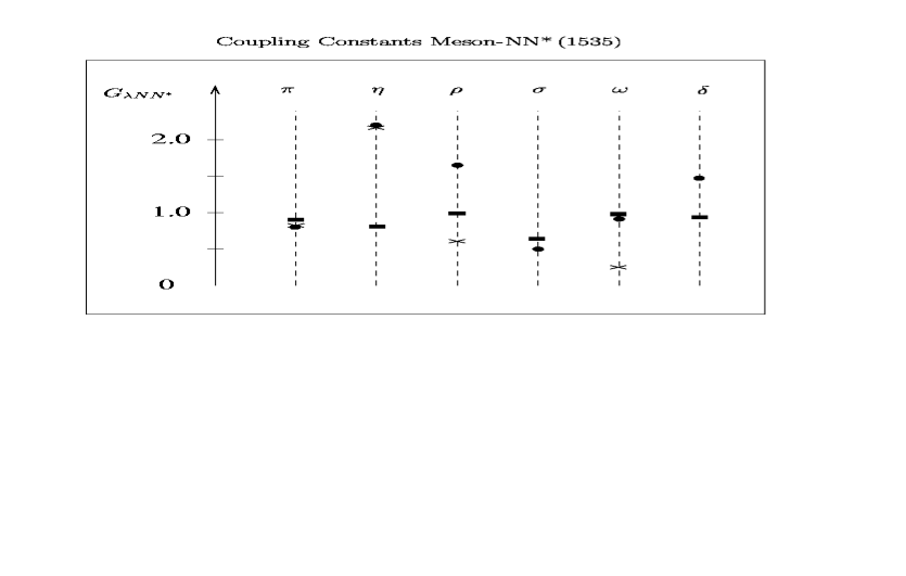
Figure 1:

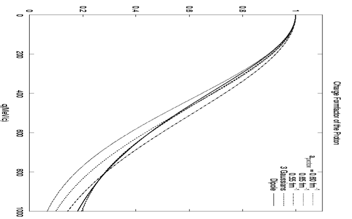
Figure 2:

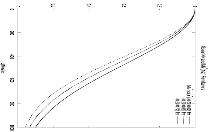
Figure 3:

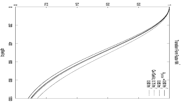
Figure 4:

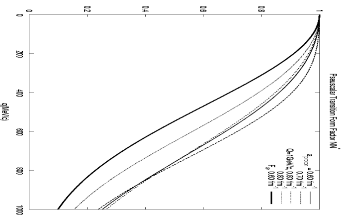
Figure 5:

References

-
[1]
T. Walcher: Nucl. Phys. A50 (2005) 185;
V. D. Burkert: Int. J. Mod. Phys. A20 (2005) 1531. -
[2]
M. Büscher et al.: Jülich FZJ, Institute for Nuclear
Physics / COSY; Annual Report 2004 , JUEL-4168 (2005) 1;
S. Kullander et al.: Nucl. Phys. A 271 (2003) 563. -
[3]
X. Shen: Nucl. Phys. Proc. Suppl. 93 (2001) 151;
W. D. Nowak: Nucl. Phys. Proc. Suppl. 105 (2002) 171;
V. Crede: Eur. Phys. J. A18 (2003) 163. -
[4]
P. Moskal et al.: Progr. Part. Nucl.
Phys. 49 (2002) 1;
C. Hanhart: Phys. Rept. 397 (2004) 155. - [5] D. E. Groom: Eur. Phys. J. C15 (2000) 1.
-
[6]
J. Smyrski et al.: Phys. Lett. B474 (2000) 182;
S. Sewerin et al.: Phys. Rev. Lett. 83 (1999) 682;
J. Aichelin and C. Hartnack: J. Phys. G27 (2001) 571. -
[7]
A. Moalem et al.: Nucl. Phys. A589 (1995) 649;
A. Moalem et al.: Nucl. Phys. A600 (1996) 445;
F. Kleefeld: Thesis, Univ. Erlangen (1999);
M. T. Pena, H. Garzilaco and D. O. Riska: Nucl. Phys. A683 (2001) 322;
G. Faeldt and C. Wilkin: Phys. Scripta 64 (2001) 427;
K. Nakayama, J. Speth and T. S. H. Lee: Phys. Rev. C65 (2002) 045210;
W. Peters, U. Mosel and A. Engel: Z. Phys. A353 (1996) 333. -
[8]
E. Gedalin, A. Moalem and L. Razdolskaja: Nucl. Phys. A634 (1998) 368;
T. Vetter et al.: Phys. Lett. B263 (1991) 153. -
[9]
F. Kleefeld and M. Dillig: Acta Phys. Polon. B29 (1998) 3059;
K. Tsushima, A. Sibirtsev and A. W. Thomas: Phys. Rev. C59 (1999) 369; Erratum-ibid. C61 (2000) 029903;
A. Sibirtsev et al.: nucl-th/0004022;
R. Shyam: Phys. Rev. C60 (1999) 055213;
R. Shyam, G. Penner and U. Mosel: Phys. Rev. C63 (2001) 022202;
A. Sibirtsev and W. Cassing: nucl-th/9904046 (Festschrift for Prof. A. Weiguny);
K. Tsushima, A. Sibirtsev and A. W. Thomas: Phys. Lett. B390 (1997) 29. -
[10]
J. F. Germond and C. Wilkin: Journ. Phys.G15 (1989) 437;
C. Wilkin: Phys. Rev. C47 (1993) 938.
-
[11]
J. J. Nagels et al.: Nucl. Phys. B147 (1979) 189;
H. J. Weber and H. Arenhövel: Phys. Rept. 36 (1978) 277;
V. Pascalutsa and R. G. E. Timmermans: Phys. Rev. C60 (1999) 042201. -
[12]
R. Machleidt: Adv. Nucl. Phys. 19 (1989) 189;
R. Machleidt: Nucl. Phys. A689 (2001) 11. -
[13]
P. Alons, M. Dillig and R. D. Bent: Nucl. Phys. A480 (1988) 413;
V. Pascalutsa: Phys. Lett. B503 (2001) 85;
S. Kondratyuk, A. D. Lahiff and H. W. Fearing: Phys. Lett. B521 (2001) 20. - [14] P. Carruthers: Introd. to Unit. Symmetry (Interscience Publ., New York; 1966).
-
[15]
M. Lutz: Inv. Talk “ Workshop Struct. Ex. Nucleons”
(Pittsburgh, USA, oct. 9-12, 2002);
G. Penner: Inv. Talk “ Workshop Struct. Ex. Nucleons” (Pittsburgh, USA, oct. 9-12, 2002). - [16] D. O. Riska and G. E. Brown: Nucl. Phys. A679 (2001) 577.
-
[17]
M. Anselmino and E. Predazzi: Proc. “Diquark 3”
(Ed. World Scientific, Singapore) (1998);
C. F. Berger. B. Lechner and W. Schweiger: Fizika B8 (1999) 371;
P. Kroll: Few Body Syst. Suppl. 11 (1999) 255. -
[18]
M. Oettel, M. Pichowsky and L. von Smekal: Eur. Phys. J.
A8 (2000) 251;
M. Oettel, R. Alkofer and L. von Smekal: Eur. Phys. J. A8
(2000) 553;
R. Alkofer and L. von Smekal: Phys. Rep. 353 (2001) 281; -
[19]
A. Amghar, B. Desplanques and L. Teussl: Nucl. Phys.
A714 (2003) 213;
M. Dillig and C. Rothleitner: preprint FAU-TP3-06/No. 09, Univ. Erlangen (2006). - [20] J. P. Elliot: Proc. Roy. Soc. A245 (1958) 128, 562.
-
[21]
F. Coester, K. Dannborn and D. O. Riska: Nucl. Phys. A634
(1998) 335;
S. Capstick and W. Roberts: Prog. Part. Nucl. Phys45; (2000) S241;
U. Löring et al.: Eur. Phys. J. A10 (2001) 395;
U. Löring et al.: Eur. Phys. J. A10 (2001) 447. - [22] L. Ya. Glozman and D. G. Riska: Phys. Lett. B366 (1996) 305.
- [23] J. D. Bjorken and S. D. Drell: Relativistic Quantum mechanics. (McGraw-Hill, Inc) (1964).
- [24] A. R. Edmonds: Angular Momentum in Quantum Mechanics. (Princeton Univ. Press, Princeton NJ) (1957).
-
[25]
J. Sakurai: Ann. Phys. 11 (1960) 1;
R. K. Bhaduri: Models of the Nucleon (Add.-Wesley, Inc.; 1987). - [26] A. W. Thomas and W. Weise: The Structure of the Nucleon (Wiley-VCA, Berlin) (2001).
-
[27]
P. A. M. Guichon: Phys. Lett. B200 (1988) 235;
K. Saito, K. Tsushima and A. W. Thomas: Phys. Lett. B406 (1997) 287. -
[28]
D. H. Lu, A. W. Thomas and A. G. Williams: Phys. Rev. C55
(1997) 3108;
D. H. Lu, A. W. Thomas and A. G. Williams: Phys. Rev. D57 (1998) 2638;
B. D. Keister and W. N. Polyzou: Adv. Nucl. Phys. 20 (1991) 225;
S. Boffi et al.: Eur. Phys. J. A14 (2002) 17. -
[29]
C. Fuchs and H. Lenske: Phys. Rev. C52 (1995) 3043;
U. Mosel: Progr. Part. Nucl. Phys. 42 (1999) 163;
M. Lutz: Nucl. Phys. A677 (2000) 241;
C. Keil, H. Lenske and C. Greiner: J. Phys. G28 (2002) 1683.