Investigation of subtreshold resonances with the Trojan Horse Method

Abstract

It is pointed out that the Trojan-Horse method is a suitable tool to investigate subthreshold resonances.

1 Transfer Reactions and Trojan Horse method

A similarity between cross sections for two-body and closely related three-body reactions under certain kinematical conditions Fuc71 led to the introduction of the Trojan-Horse method Bau86 ; Typ00 ; tyba02 . In this indirect approach a two-body reaction

$$A+x\to C+c$$ (1)

that is relevant to nuclear astrophysics is replaced by a reaction

$$A+a\to C+c+b$$ (2)

with three particles in the final state. One assumes that the Trojan horse $a$ is composed predominantly of clusters $x$ and $b$, i.e.  $a=(x+b)$. This reaction can be considered as a special case of a transfer reaction to the continuum. It is studied experimentally under quasi-free scattering conditions, i.e. when the momentum transfer to the spectator $b$ is small. The method was primarily applied to the extraction of the low-energy cross section of reaction (1) that is relevant for astrophysics. However, the method can also be applied to the study of single-particle states in exotic nuclei around the particle threshold. The basic assumptions of the Trojan Horse Method are discussed in detail in tyba02 , see also mukha .

It is the purpose of this contribution to study the transition from the bound ($E_{Ax}<0$) to the unbound ($E_{Ax}>0$) region. We study the case where there is an open channel $c+C\neq A+x$ at the $E_{Ax}=0$ threshold. We show that there is a continuous transition. If there is a subthreshold resonance in the $B=A+x$-system it can be experimentally studied in the $A+(b+x)\rightarrow C+c+b$ reaction.

2 Continuous Transition from Bound to Unbound State Stripping

For the case where only the elastic channel $A+x$ is open we refer to Ch. 4.2.1 of msuproc . Now we study the case where the reaction $x+A\rightarrow C+c$ has a positive $Q$ value, the relative energy $E$ between A and x can be negative as well as positive in the three-body reaction $A+a(=b+x)\rightarrow C+c+b$. As an example we quote the recently studied Trojan horse reaction $d+^{6}Li\rightarrow\alpha+^{3}He+n$ auro03 applied to the ⁶Li$(p,\alpha)^{3}$He two-body reaction (the neutron being the spectator). In this case there are two charged particles in the initial state (⁶Li+$p$) and the $\alpha+^{3}$He-channel is open at the $E=E_{{}^{6}Li+p}=0$-threshold.

The general question which we want to answer here is how the two regions $E>0$ and $E<0$ are related to each other. In fig.1

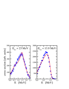
Figure 1: The double differential cross section of the Trojan horse reaction $d+^{6}Li\rightarrow\alpha+^{3}He+n$ is finite at the $p+^{6}Li$ relative energy $E=0$. How does it continue to energies $E<0$?

(fig.7 of auro03 ) the coincidence yield is plotted as a function of the ⁶Li-$p$ relative energy $E$. It is nonzero at zero relative energy. How does the theory tyba02 (and the experiment) continue to negative relative energies? With this method, subtreshold resonances can be investigated rather directly.

The cross section is a quantity which only exists for $E>0$. However, a quantity like the S factor (or related to it) can be continued to energies below the threshold. An instructive example is the modified shape function $\tilde{S}$ in Ch. 6 of tyba04 . In analogy to the astrophysical S factor, where the Coulomb barrier is taken out, the angular momentum barrier is taken out in $\tilde{S}$. As can be seen from table 3 or 4 of tyba04 $\tilde{S}$ is well defined for $x^{2}<0$, with the characteristic pole at $x^{2}=-1$, corresponding to the binding energy of the $(A+x)=B$-system.

The inclusive breakup theory of IAV iav ; mun is extended to negative energies $E<0$ in msuproc . We refer the reader to this reference for this approach.

An alternative approach is based directly on the formulation of tyba02 . The Trojan horse cross section is given in eq.(61) there. The S-matrixelement $S_{AxCc}$ can be found from the asymptotics of the radial wave functions, see eq. (23) there. For negative energies $E<0$ the channel is closed and the outgoing wave function is replaced by an exponentially decaying one. The quantity $S_{AxCc}$ then is no longer an S-matrixelement, but it plays the role of a normalization constant, see also wigner ; lanethom .

The Trojan horse amplitude involves the combination $f\propto S_{lc}\cdot J^{+}_{l}$ (see eq. (61) of tyba02 . The threshold behaviour of $J^{+}$ in the case of neutrons is given by A.30, for charged particles by eq. 59 of tyba02 . The energy behaviour of the inelastic $cC\neq Ax$ S-matrixelement is found from the behaviour of the elastic S-matrixelement $S_{ll}$ and unitarity: $|S_{lc}|^{2}=1-|S_{ll}|^{2}$ where $l\neq c$. We have $S_{ll}=\exp 2i\delta_{l}\sim 1-2i\delta_{l}^{R}-2\delta_{l}^{I}$, where the imaginary part of the phase shift goes like $\delta_{l}^{I}\sim(kR)^{2l+1}$ for neutral particles. This leads to $|S_{lc}|^{2}\sim(kR)^{2l+1}$. The product $S_{lc}\cdot J_{l}^{+}$ is given by $|S_{lc}J_{l}^{+}|^{2}\sim(kR)^{3}$ and the cross section $\sigma\propto\frac{1}{k^{3}}|S_{lc}J_{l}^{+}|^{2}$ tends to a finite constant independent of k. A similar analysis can be done for charged particles.

We now study the smooth change from $E>0$ to $E<0$ in a two-channel model with a surface coupling. For the case of $l=0$ it was studied in Ch. 4.2.3 of msuproc . Two radial functions $f_{1}$ and $f_{2}$ (we assume the same l-value) are coupled by a potential of the type $u_{ij}(r)f_{j}(r)$. We take $u_{ij}=Q\delta(r-R)$. We are especially interested in the case where there is a resonance just below or above the threshold of channel 1$\equiv(A+x)$, channel 2 ($\equiv C+c)$ is always open.

In the channel 1 the wave function is $\zeta=Nu_{l}^{+}(iqr)$, for $E<0$ and $\zeta=Su_{l}^{+}(kr)$, for $E>0$. The in- and outgoing wave functions are given by $u_{l}^{\pm}=e^{\mp i\sigma_{l}}(G_{l}\pm iF_{l})\rightarrow\exp(\pm i(kr-\eta ln(2kr)-\frac{l\pi}{2}))$. For $E<0$ they correspond to exponentially decreasing and increasing wave functions. The logarithmic derivative in this channel is independent of $S$ or $N$. For $r\geq R$ the radial wave functions are given in terms of the S-matrix-elements by

$$f_{1}=\sqrt{k_{2}/k_{1}}\frac{1}{2i}S_{12}u_{l}^{+}(k_{1}r)$$ (3)

and

$$f_{2}=\frac{1}{2i}(S_{22}u_{l}^{+}(k_{2}r)-u_{l}^{-}(k_{2}r))$$ (4)

The logarithmic matching conditions lead to a ’Sprungbedingung’, which determines the S-matrixelements. Denoting the interior logarithmic derivatives ($L\equiv\frac{rf{{}^{\prime}}}{f}$) by $L_{1}$ and $L_{2}$ we have

$$\frac{Rf_{1}^{{}^{\prime}}(R_{>})}{f_{1}(R_{>})}\equiv q_{l}^{+}(\kappa_{1})=L_{1}+QR\frac{f_{2}(R)}{f_{1}(R)}$$ (5)

and

$$\frac{Rf_{2}^{{}^{\prime}}(R_{>})}{f_{2}(R_{>})}=L_{2}+QR\frac{f_{1}(R)}{f_{2}(R)}$$ (6)

where $\kappa_{1}\equiv k_{1}R$. Eq. (5) can be solved for $f_{1}$. The LHS is a ’kinematic ’ quantity, it is given by $q_{l}^{+}\equiv\frac{\kappa u_{l}^{+^{\prime}}}{u_{l}^{+}}$ and we have

$$f_{1}(R)=\frac{QRf_{2}}{q_{l}^{+}(\kappa_{1})-L_{1}}$$ (7)

For the case of neutral particles (neutrons) we have the following behaviour close to threshold : $\rm{Re}q_{l}^{+}=-l+O(k^{2})$ and $\rm{Im}q_{l}^{+}\sim(\kappa_{1})^{2l+1}/((2l-1)!!)^{2}\equiv s_{l}\equiv\kappa_{1}v_{l}$. The penetration factor $s_{l}$ is a small number. Charged particles can be treated in an analogous way. Inserting into eq.(9) we obtain an equation for the unknown S-matrixelement $S_{22}$:

$$\kappa_{2}\frac{S_{22}\frac{du_{l}^{+}}{d\kappa_{2}}-\frac{du_{l}^{-}}{d\kappa_{2}}}{S_{22}u_{l}^{+}-u_{l}^{-}}=L_{2}+\frac{(QR)^{2}}{q_{l}^{+}(\kappa_{1})-L_{1}}\equiv\tilde{L_{2}}$$ (8)

where $\kappa_{2}\equiv k_{2}R$. This equation can be solved for $S_{22}$, we write $S_{22}=\exp(2i\tau_{l})S_{22}^{res}$, where $\tau_{l}$ is the hard sphere phase shift. We find

$$S_{22}^{res}=\frac{\tilde{L_{2}}-q_{l}^{-}(\kappa_{2})}{\tilde{L_{2}}-q_{l}^{+}(\kappa_{2})}$$ (9)

If channel 1 is closed, $q_{l}^{+}(\kappa_{1})$ is real, thus $\tilde{L_{2}}$ is real and one obtains the form of a single particle resonance with appropriate parameters. The S-matrix is $1\times 1$ and $S_{22}$ is unitary. If channel 1 is open: $\tilde{L_{2}}$ is complex and we can bring $S_{22}^{res}$ in a two-channel Breit- Wigner resonance form. $S_{12}$ is then obtained (for a closed or an open channel 1) from eqs. 3 and 7.

Although our model is quite special, the resulting form has a general validity, with (’effective’) resonance parameters $E_{R}$ (position) and partial widths $\Gamma_{1},\Gamma_{2}$. The total width is $\Gamma=\Gamma_{1}+\Gamma_{2}$. It is a merit of our model that it shows directly how $S_{12}$ is extended to closed channels. It will be interesting to elucidate the relation of the present model to the more general approach of Ref. mutri .

The standard Breit-Wigner result is (see e.g.rr )

$$S_{ij}=\exp{i(\xi_{i}+\xi_{j})}(\delta_{ij}-\frac{i\sqrt{\Gamma_{i}\Gamma_{j}}}{E-E_{R}+i\Gamma/2})$$ (10)

We now show how to obtain these forms from the coupled channel model. The condition for a resonance at position $E_{R}$ is $\rm{Re}\tilde{L_{2}}-\rm{Re}q_{l}^{+}(E_{R})=0$: This defines $E_{R}$. In the resonance energy region we can write $\rm{Re}\tilde{L_{2}}-\rm{Re}q_{l}^{+}=-c_{3}(E-E_{R})$ where $c_{3}$ is some constant. The partial widths $\Gamma_{1}$ and $\Gamma_{2}$ are found from $\frac{1}{2}(\Gamma_{1}+\Gamma_{2})\equiv\frac{-1}{2c_{3}}(\rm{Im}\tilde{L_{2}}-\rm{Im}q_{l}^{+}(\kappa_{2,R}))$ and $\frac{1}{2}(\Gamma_{1}-\Gamma_{2})\equiv\frac{-1}{2c_{3}}(\rm{Im}\tilde{L_{2}}-\rm{Im}q_{l}^{-}(\kappa_{2,R}))$. We assume that we have a single particle resonance in the uncoupled channel 2, whereas there is no resonance structure in channel 1 (i.e. $\rm{Re}q_{l}^{+}-L_{1}$ is different from zero). The ’bare’ resonance condition is $L_{2}(=\rm{real})=\rm{Re}q_{l}^{+}(\kappa_{2})$. The coupling induces a shift of the resonance energy.

We have $\rm{Im}q_{l}^{+}=-\rm{Im}q_{l}^{-}(\kappa)=s_{l}(\kappa)$. Since $s_{l}(\kappa_{1})<<1$ we have $\rm{Im}\tilde{L_{2}}=\frac{-(QR)^{2}s_{l}}{(l+L_{1})^{2}}$. We obtain

$$\Gamma_{1}=\frac{2s_{l}(\kappa_{1})(QR)^{2}}{c_{3}(l+L_{1})^{2}}$$ (11)

and

$$\Gamma_{2}=\frac{2s_{l}(\kappa_{2})}{c_{3}}$$ (12)

Thus the Breit-Wigner form of $S_{22}$ is recovered. We see that $\Gamma_{1}$ is strongly energy dependent: it contains the threshold penetration factor $s_{l}(\kappa_{1})$, whereas $\Gamma_{2}$ (and thus also the total width $\Gamma$) do not. For $E\leq 0$ the S-matrix consists only of $S_{22}$, which is unitary. Still, $S_{12}$ which now plays the role of a normalization factor is nonzero.

By direct calculation we can bring $S_{12}$ in the Breit-Wigner form: We write $f_{2}(\kappa_{2})=S_{22}u_{l}^{+}-u_{l}^{-}=u_{l}^{-}(S_{22}^{res}-1)$. From eqs. (3,4) and (7) we find

$$S_{12}=\sqrt{k_{1}/k_{2}}\frac{-QRu_{l}^{-}(\kappa_{2})}{u_{l}^{+}(\kappa_{1})(l+L_{1})}\frac{-i\Gamma_{2}}{E-E_{R}+\frac{i}{2}(\Gamma_{1}+\Gamma_{2})}=e^{i(\tau_{1}+\tau_{2})}\frac{-i\sqrt{\Gamma_{1}\Gamma_{2}}}{E-E_{R}+\frac{i}{2}(\Gamma_{1}+\Gamma_{2})}$$ (13)

We used eqs. (11) and (12), $u_{l}^{\pm}=\frac{1}{\sqrt{v}_{l}}e^{\mp i\tau_{l}}$ and $s_{l}\equiv\kappa v_{l}$to obtain this result.

This result is valid for $E>0$. For $E<0$ there are some simple modifications. The wave number becomes imaginary, $k=iq$. The quantity $q_{l}^{\pm}$ is real, $u_{l}^{+}$ can again be written as $1/\sqrt{v_{l}}\exp{\frac{-i\pi l}{2}}$(for neutral particles). Thus we have $\tau_{1}=\frac{i\pi l}{2}$ for $E<0$. Formally, the penetration factor $s_{l}$ turns imaginary ($s_{l}=i(-1)^{2l}(qR)^{2l+1}/((2l-1)!!)^{2})$, and so does the width $\Gamma_{1}$, see eq. (11).

For $E_{R}>0$ we have a resonance, for $E_{R}<0$ a subthreshold resonance, the formulae are valid for both cases. The opening of channel 1 at threshold will induce cusp effects in the elastic $C+c\rightarrow C+c$ scattering, see e.g. newton .

2.1 Large $p_{1/2}$-scattering length in the ¹¹Be system due to a neutron halo state

The electromagnetic dipole strength in ¹¹Be was deduced tybaprl from high-energy ¹¹Be Coulomb dissociation messurements at GSI palit . Using a cutoff radius of $R=2.78$ fm and an inverse bound-state decay length of $q=0.1486$ fm^-1 as input parameters we extract an ANC of $C_{0}=0.724(8)$ fm^-1/2 from the fit to the experimental data. The ANC can be converted to a spectroscopic factor of $C^{2}S=0.704(15)$ that is consistent with results from other methods. In the lowest order of the effective-range expansion the phase shift $\delta_{l}^{j}$ in the partial wave with orbital angular momentum $l$ and total angular momentum $j$ is written as $\tan\delta_{l}^{j}=-a_{l}k^{2l+1}=-(xc_{l}^{j}\gamma)^{2l+1}$, where $\gamma=qR=0.4132<1$ is the halo expansion parameter and $x=k/q=\sqrt{E/S_{n}}$. The neutron separation energy is $S_{n}$. The parameter $c_{l}^{j}$ corresponds to the scattering length $a_{l}^{j}=(c_{l}^{j}R)^{2l+1}$. We obtain $c^{3/2}_{1}=-0.41(86,-20)$ and $c^{1/2}_{1}=2.77(13,-14)$. The latter is unnaturally large because of the existence of a bound $\frac{1}{2}^{-}$ state close to the neutron breakup threshold in ¹¹Be.

The connection of the scattering length $a_{l}$ and the bound state parameter q for $l>0$ is given by $a_{l}=\frac{2(2l-1)R^{2l-1}}{q^{2}(2l+1)!!(2l-1)!!}$, where a square well potential model with a range R was assumed. This is a generalization of the well-known relation $a_{0}=1/q$ for $l=0$. The $p_{1/2}$ channel in ¹¹Be is an example for the influence of a halo state on the continuum. The binding energy of this state is given by 184 keV, which corresponds to $q=0.094$ fm. With $R=2.78$ fm one has $\gamma^{2}=0.068$. For $l=1$ one has $a_{1}=\frac{2R^{3}}{3\gamma^{2}}=210$  fm³ which translates into $c_{1}=(a_{1}/R^{3})^{1/3}=2.14$. This compares favourably with the fit value given in table 1 of tybaprl : $2.77(13,-14)$. The corresponding scattering length is given by $a_{1}^{1/2}=457(67,-66)fm^{3}$. For a further discussion we refer to tybaprl . The large $p_{1/2}$-scattering length would also manifest itself in the ${}^{10}Be(d,p\gamma)^{11}Be$ ’radiative transfer reaction’.

3 Conclusion and Outlook

The treatment of the continuum is a general problem, which becomes more and more urgent when the dripline is approached. We studied the transition from bound to unbound states as a typical example. In the present analysis this transition is continuous, it is expected that this also shows up in the experimental data. A minireview of the applications of the Trojan horse method to astrophysical reactions can be found in mumbai An extension to stripping into the continuum would be of interest for this and other kinds of reactions. The trojan horse reaction ${}^{18}F(d,n\alpha)^{15}O$ would be of great interest for the ${}^{18}F(p,\alpha)^{15}O$ reaction relevant for nova nucleosynthesis nucnews ; hribf . This would also be of interest for SPIRAL2, for example. Another most interesting example would be the radiative $\alpha$-transfer reaction ${}^{12}C(^{6}Li,d\gamma)^{16}O$, where one could also look directly for the subtreshold $1^{-}$ and $2^{+}$ states which are crucial for the S-factor of the astrophysically important $\alpha$-capture reaction ${}^{12}C(\alpha,\gamma)^{16}O$.

References

• (1) H.ย Fuchs et al., Phys. Lett. B, 37, 285 (1971).
• (2) G.ย Baur, Phys. Lett. B, 178, 135 (1986).
• (3) S.ย Typel and H.ย H.ย Wolter, Few Body Systems, 29, 75 (2000).
• (4) S.ย Typel and G.ย Baur, Ann. Phys., 305, 228 (2003).
• (5) A.ย M.ย Mukhamedzhanov, C.ย Spitaleri, R.ย E.ย Tribble, nucl-th/0602001
• (6) G.ย Baur, S.ย Typel nucl-th/0504068, Proceedings of the Workshop on โ€Reaction Mechanisms for Rare Isotope Beamsโ€, Michigan State University, March 9-12, 2005.
• (7) A.ย Tumino et al., Phys. Rev. C, 67, 065803 (2003).
• (8) S.ย Typel and G.ย Baur, Nucl. Phys. A759, 247 (2005), nucl-th/0411069.
• (9) M.ย Ichimura, N.ย Austern, and C.ย M.ย Vincent, Phys. Rev. C, 32, 431 (1985).
• (10) M.ย Ichimura, Phys. Rev. C, 41, 834 (1990).
• (11) A.ย M.ย Lane and R.ย G.ย Thomas Rev. Mod. Phys. 30(1958)257
• (12) E.ย P.ย Wigner, Phys. Rev., 73, 1002 (1948).
• (13) A.ย M.ย Mukhamedzhanov and R.ย E.ย Tribble, Phys. Rev. C, 59, 3418 (1999)
• (14) C.ย E.ย Rolfs and W.ย S.ย Rodney, Cauldrons in the Cosmos (The University of Chicago Press, Chicago, 1988)
• (15) R.ย G.ย Newton, Scattering Theory of Waves and Particles, McGraw-Hill, New York, 1966
• (16) S.ย Typel and G.ย Baur, Phys. Rev. Lett., 93, 142502 (2004).
• (17) R.ย Palit et al., Phys. Rev. C, 68, 034318 (2003).
• (18) J.ย Jose and A.ย Coc Nuclear Physics News Vol.15,No.4,2005 p.17
• (19) G.ย Baur and S.ย Typel nucl-th/0601004, Proceedings of the DAE-BRNS 50th Symposium on Nuclear Physics, Bhabha Atomic Research Centre, Mumbai, India December 12-16, 2005
• (20) J.ย C.ย Blackmon J. Phys. G 31 (2005) S1405