Near–Fields and Initial Energy Density in High Energy Nuclear Collisions

Abstract

We calculate the classical gluon field created at early times in collisions of large nuclei at high energies. We find that the field is dominated by the longitudinal chromoelectric and chromomagnetic components. We estimate the initial energy density of this gluon field to be approximately 260 GeV/fm³ at RHIC.

Experiments are being carried out at the Relativistic Heavy Ion Collider (RHIC) and soon will be at the CERN Large Hadron Collider (LHC) to create and study quark gluon plasma. Data from RHIC indicate that in collisions of gold nuclei at $\sqrt{s_{NN}}=200$ GeV energy densities far in excess of the critical value required for deconfinement ($\epsilon_{c}\approx 2$ GeV/fm³) are reached rhic-wp . Furthermore, the partonic phase seems to be thermalized after a very short time $\tau_{0}<1$ fm/$c$. While the evolution of the quark gluon plasma in equilibrium can be described by relativistic hydrodynamics KH , the initial soft interactions of the nuclei and the thermalization process before the time $\tau_{0}$ are still not completely understood.

It has been argued that the initial dynamics for the collision of two very high energy nuclei is determined by a universal phase called the color glass condensate (CGC). This idea is based on gluon saturation at a scale $~{}Q_{s}$ MV ; KMW ; JMKMLW:96 ; cgc ; McL:05 . Slowly evolving and randomly distributed color charges in the nuclei are the sources of this gluon field. A simple implementation is the McLerran-Venugopalan (MV) model MV ; KMW in which the gluon field is given by the solution of the classical Yang-Mills equations.

In this Letter we calculate the gluon field at early times after the collision in the framework of the McLerran-Venugopalan model. We use an expansion of the Yang-Mills equations in powers of the proper time $\tau$. This is a near–field approximation which may be the most appropriate use of the color glass condensate picture. We also estimate the initial energy density at the time of overlap of the nuclei using a simple model for the nuclear gluon distribution and coarse-graining methods to avoid ultraviolet (UV) singularities. More details and a discussion of applications will be provided elsewhere FKLMB .

In high energy collisions the two colliding nuclei are highly Lorentz contracted; therefore, the valence and large-$x$ partons are described by infinitesimally thin sheets propagating on the light cone. Although each nucleus is color neutral as a whole, local color fluctuations do occur. At the moment of overlap, the color distributions in nucleus 1 ($+$ light cone) and 2 ($-$ light cone) are $\rho_{1}(\mathbf{x}_{\perp})$ and $\rho_{2}(\mathbf{x}_{\perp})$, respectively. We use light cone coordinates $x^{\pm}=\left(x^{0}\pm x^{3}\right)/\sqrt{2}$ and ${\bf x}_{\perp}=(x^{1},x^{2})$. The distributions $\rho_{k}=\rho_{k}^{a}t^{a}$ ($k=1,2$) are functions with values in $SU(3)$. Since they resemble fluctuations of color we have to take the ensemble average of all allowed functions $\rho_{k}$ at the end. It is convenient to choose an axial gauge defined by $A^{+}x^{-}+A^{-}x^{+}=0$. In this gauge the current generated by the charges $\rho_{k}$ takes the form $J^{\pm}=\delta(x^{\mp})g\rho_{1,2}({\bf x}_{\perp})$ and $J^{i}=0$, satisfying the equation of continuity $\left[D_{\mu},J^{\mu}\right]=0$. The gluon field generated by this current can be obtained by solving the Yang-Mills equations $[D_{\mu},F^{\mu\nu}]=J^{\nu}$.

The gauge potential $A^{\mu}$ is a smooth function of $x^{\mu}$ except for lines with propagating charge. We follow the authors of ref. KMW who showed that the ansatz

$$A^{\pm}(x) = \pm\theta(x^{+})\theta(x^{-})x^{\pm}\alpha(\tau,{\bf x}_{\perp})\,,$$ (1)

$$A^{i}(x) = \theta(x^{-})\theta(-x^{+})\alpha_{1}^{i}({\bf x}_{\perp})+\theta(x^{+})\theta(-x^{-})\alpha_{2}^{i}({\bf x}_{\perp})$$ (2)

$$+ \theta(x^{+})\theta(x^{-})\alpha_{3}^{i}(\tau,{\bf x}_{\perp})\,.$$

satisfies the Yang-Mills equations in the different sectors of Minkowski space. Here upper Latin indices $i$, $j$, $\ldots$ always refer to transverse components. The $\alpha_{1}^{i}$ and $\alpha_{2}^{i}$ are the purely transverse gauge potentials of nucleus 1 and 2, respectively. They can be written with the help of transformation matrices $U_{k}=e^{i\phi_{k}}$, $k=1,2$, such that they are gauge transformations of the vacuum:

$$\alpha_{k}^{i}({\bf x}_{\perp}) =\frac{i}{g}U^{-1}_{k}\partial^{i}U_{k}\,\text{, with}$$ (3)

$$\nabla_{\perp}^{2}\phi_{k}(\mathbf{x}_{\perp}) =g^{2}\rho_{k}(\mathbf{x}_{\perp}).$$ (4)

$\alpha$ and $\alpha_{3}^{i}$ describe the field in the forward light cone ($x^{+}>0$, $x^{-}>0$) which is generated in the collision. They are smooth functions of $\mathbf{x}_{\perp}$ and the proper time $\tau=\sqrt{2x^{+}x^{-}}$. They are independent of the space-time rapidity $\eta=1/2\ln(x^{+}/x^{-})$ because the current $J^{\mu}$ is boost-invariant. In the forward light cone the Yang-Mills equations can be rephrased as KMW :

$$\frac{1}{\tau^{3}}\partial_{\tau}\tau^{3}\partial_{\tau}\alpha-[D^{i},[D^{i},\alpha]] =0\,,$$ (5)

$$\frac{1}{\tau}[D^{i},\partial_{\tau}\alpha^{i}_{3}]-ig\tau[\alpha,\partial_{\tau}\alpha] =0\,,$$ (6)

$$\frac{1}{\tau}\partial_{\tau}\tau\partial_{\tau}\alpha^{i}_{3}-ig\tau^{2}[\alpha,[D^{i},\alpha]]-[D^{j},F^{ji}] =0\,.$$ (7)

$\alpha$ and $\alpha_{3}^{i}$ are connected with the single nucleus fields $\alpha^{i}_{1,2}$ via boundary conditions at $\tau=0$:

$$\alpha_{3}^{i}(\tau=0,{\bf x}_{\perp}) = \alpha_{1}^{i}({\bf x}_{\perp})+\alpha_{2}^{i}({\bf x}_{\perp})\,,$$ (8)

$$\alpha(\tau=0,{\bf x}_{\perp}) = -\frac{ig}{2}\left[\alpha_{1}^{i}({\bf x}_{\perp}),\alpha_{2}^{i}({\bf x}_{\perp})\right]\,.$$ (9)

An explicit analytic solution of (5)–(7) is not known. However, lowest order perturbative solutions KMW as well as numerical solutions KV:98 ; Lappi:03 are available.

Decoherence and pair production GKT:05 ; KharTuch:05 will eventually destroy the classical field and lead to thermalization. Typical values for the thermalization time $\tau_{0}$ used in hydrodynamic calculations range from 0.15 fm/$c$ to 1.0 fm/$c$ rhic-wp ; KH . It is clear that the classical description breaks down before $\tau_{0}$. Hence, what we can hope to calculate in this particular framework is the short-term behavior of the gluon field, i.e. the near-field close to the light cone. The functions $\alpha$ and $\alpha_{3}^{i}$ are regular at $\tau=0$. Therefore it is legitimate to solve the Yang-Mills equations using a power series in $\tau$. We write

$$\alpha(\tau,{\bf x}_{\perp})=\sum_{n=0}^{\infty}\tau^{n}\alpha_{(n)}({\bf x}_{\perp})\,,$$ (10)

and similarly for $\alpha_{3}^{i}$. We also use expansions for the field strength tensor and covariant derivative in the forward light cone with coefficients $F^{\mu\nu}_{(n)}$ and $D^{\mu}_{(n)}$, respectively.

Using these expansions in Eqs. (5) through (7) yields an infinite set of equations for the coefficients $\alpha_{(n)}$ and $\alpha_{3(n)}^{i}$. To lowest order in $\tau$, the fields are just given by the boundary conditions (8) and (9),

$$\alpha^{i}_{3(0)} =\alpha_{1}^{i}+\alpha_{2}^{i}\,,$$ (11)

$$\alpha_{(0)} =-ig[\alpha_{1}^{i},\alpha_{2}^{i}]/2\,.$$ (12)

It is now possible to give a solution for any order in $\tau$ recursively. It is straightforward to prove that for $n>1$

$$\alpha_{(n)} =\frac{1}{n(n+2)}\sum_{k+l+m=n-2}\left[D^{i}_{(k)},[D^{i}_{(l)},\alpha_{(m)}]\right]\,,$$

$$\alpha^{i}_{3(n)} =\frac{1}{n^{2}}\left(\sum_{k+l=n-2}\left[D^{j}_{(k)},F^{ji}_{(l)}\right]\right.$$ (13)

$$\quad\left.+ig\sum_{k+l+m=n-4}\left[\alpha_{(k)},[D^{i}_{(l)},\alpha_{(m)}]\right]\right).$$

One can immediately conclude that these fields vanish for all odd powers of $\tau$: $\alpha_{(2n+1)}=0$, $\alpha_{3(2n+1)}^{i}=0$. Similar recursion relations hold for the field strength tensor. For brevity we only cite the relation for the longitudinal chromoelectric field $E_{z}=F^{+-}$ which is

$$F^{+-}_{(n)}=\sum_{k+l+m=n-2}\frac{1}{n(m+2)}\left[D^{i}_{(k)},[D^{i}_{(l)},F^{+-}_{(m)}]\right]\,.$$ (14)

A summation of the recursive solution in closed form does not seem feasible. However, we assert that an analysis using just the first few orders in $\tau$ is extremely useful.

The non-vanishing components of the field strength for the lowest three orders in $\tau$ are

$$F^{+-}_{(0)} =ig\left[\alpha_{1}^{i},\alpha_{2}^{i}\right]\,,$$ (15)

$$F^{21}_{(0)} =ig\epsilon^{ij}\left[\alpha_{1}^{i},\alpha_{2}^{j}\right]\,,$$ (16)

$$F^{i\pm}_{(1)} =-\frac{e^{\pm\eta}}{2\sqrt{2}}\left([D^{j}_{(0)},F^{ji}_{(0)}]\pm[D^{i}_{(0)},F^{+-}_{(0)}]\right)\,,$$ (17)

$$F^{+-}_{(2)} =\frac{1}{4}[D^{i}_{(0)},[D^{i}_{(0)},F^{+-}_{(0)}]]\,,$$ (18)

$$F^{21}_{(2)} =\frac{1}{4}[D^{i}_{(0)},[D^{i}_{(0)},F^{21}_{(0)}]]\,.$$ (19)

Here $\epsilon^{ij}$ is the antisymmetric tensor. Thus the longitudinal chromoelectric field $E_{z}$ and the longitudinal chromomagnetic field $B_{z}=F^{21}$ start with finite values at $\tau=0$. The transverse electric and magnetic fields, which are linear combinations of the components $F^{i\pm}$, are zero at $\tau=0$ and start at order $\tau^{1}$. Generally, longitudinal fields have only contributions from even powers in $\tau$, transverse fields only consist of odd powers in $\tau$.

This observation leads to the following space-time picture. Inside the nuclei the color sources create purely transverse fields $F^{i\pm}=\delta(x^{\mp})\alpha_{1,2}^{i}$ on the light cone. This is completely analogous to the abelian case. After nuclear overlap, non-abelian interactions between these fields create strong longitudinal chromoelectric and chromomagnetic fields, while the onset of transverse fields in the forward light cone is delayed. The situation resembles a capacitor with a longitudinal field, but it is important to realize that only the non-abelian nature of the gluon field can generate such a field for recoilless charges receding from each other with the speed of light. The strong longitudinal fields at early times are an immediate consequence of the equations of motion; however, this fact has not received much attention before. Recently the strong pulse of longitudinal fields and its possible consequences have been discussed FKL:05 ; KharTuch:05 ; KhaVen:01 ; LaMcL:06 .

In the second part of this Letter we would like to use our results to discuss the initial energy density $\epsilon_{0}=\langle T^{00}_{(0)}\rangle$ for $\tau\to 0$. Here $T^{\mu\nu}$ is the energy momentum tensor of the classical field which we expand in powers of $\tau$ as well. We postpone all further discussion to a later publication FKLMB . Note that the recursion formulas use the gluon fields $\alpha^{i}_{k}$ as the starting point. However those have to be determined by solving the Yang-Mills equations (3), (4) for a single nucleus which is a difficult task. For our discussion here, difficulties associated with non-linearities in the boundary conditions are simplified by a mean-field approximation. As we will argue below it still represents the essential physics of the full solution. We achieve this by replacing Eqs. (3) and (4) with

$$\left(\nabla^{2}_{\perp}-\frac{1}{R_{c}^{2}}\right)\phi_{k}=g^{2}\rho_{k}\,,\quad\alpha_{k}^{i}=-\frac{1}{g}\partial^{i}\phi_{k}\,.$$ (20)

The solution is formally linear in $\rho_{k}$. However, we introduced a screening length $R_{c}$ as a parameter which will depend on the charge distribution $\rho_{k}$.

The idea behind this approximation to Eqs. (3) and (4) is as follows. To lowest order in the charge density $\rho_{k}$ we have $\alpha_{k}^{i}=-(1/g)\partial^{i}\phi_{k}+\mathcal{O}(\rho_{k}^{3})$. The primary effect of the non-linearities is a partial screening of the field on length scales $\sim 1/Q_{s}$ JMKMLW:96 . However, the screening is incomplete unless confinement is enforced in addition LamMa:99 . In our approximation screening is provided by the scale $R_{c}\sim 1/Q_{s}$ and the result is perfectly infrared safe. For a reasonable estimate of the screening effect one can invoke the analogy to electric screening in a QCD plasma which implies $R_{c}^{-2}=4\alpha_{s}\sigma/3$ where $\sigma$ is the area density of the number of color charges.

Let us now consider the two nuclei as being made up of two ensembles of discrete charges, given by $SU(3)$ matrices $T_{1,u}$ and $T_{2,u}$ at transverse positions $\mathbf{b}_{u}$. The charge densities can be written as

$$\rho_{k}(\mathbf{x}_{\perp})=\sum_{u}R(|\mathbf{x}_{\perp}-\mathbf{b}_{u}|)T_{k,u}\,.$$ (21)

The index $u$ represents coarse–grained cells in both nuclei with a certain number of color sources, $N_{1,u}$ and $N_{2,u}$, respectively, in each of them, and $R(r)$ is the spatial distribution of the effective color charge in each cell normalized to one. Note that the factorization of spatial and color degrees of freedom makes sense if the coarse-grained cells have sizes much smaller than $1/Q_{s}$.

Then from Eqs. (3), (4) it follows that the gauge potentials can be written as

$$\alpha^{i}_{k}(\mathbf{x}_{\perp})=g\sum_{u}\frac{x_{\perp}^{i}-b_{u}^{i}}{|\mathbf{x}_{\perp}-\mathbf{b}_{u}|}\tilde{T}_{k,u}G(|\mathbf{x}_{\perp}-\mathbf{b}_{u}|)$$ (22)

where $G$ is the linear field of a single charge, i.e. $G(r)=d\varphi/dr$ with $\nabla^{2}_{\perp}\varphi(r)=R(r)$. The $\tilde{T}_{k,u}$ are $SU(3)$ valued functions and can be interpreted as the modifications of the charges $T_{k,u}$ through non-linear interactions. One can expand $\tilde{T}_{k,u}(r)=T_{k,u}+\mathcal{O}(T^{3})$, where the first term is the linear contribution, and higher order terms reflect the screening from interactions with charges in neighboring cells. We can now simplify the situation by applying the approximation (20). It amounts to the replacement $\tilde{T}_{k,u}G\to T_{k,u}\tilde{G}$. The screening present in $\tilde{T}$ is now factorized into a modified field profile $\tilde{G}$ with

$$\left(\nabla^{2}_{\perp}-\frac{1}{R_{c}^{2}}\right)\tilde{\varphi}(r)=R(r)\,,\quad\tilde{G}(r)=d\tilde{\varphi}/dr\,.$$ (23)

In addition, we have to impose an ultraviolet (UV) cutoff $Q_{0}$. The McLerran-Venugopalan model does not provide a UV finite answer for the energy density at $\tau=0$, as also noticed in Lappi:06 . This comes from the fact that hard modes with momentum much larger than $Q_{s}$ are treated correctly. They are better described by hard perturbative processes. Therefore $Q_{0}$ should be chosen to be the cutoff between hard processes involving modes with transverse momentum $p_{T}>Q_{0}$, and the bulk modes with $p_{T}<Q_{0}$. We realize that our coarse-graining provides this cutoff. To be more precise we choose Gaussian profiles $R$ for each charge with a width $\lambda=1/Q_{0}$. Putting everything together we find the modified field profile is approximately

$$\tilde{G}(x_{\perp})\approx\frac{1-\exp(-x_{\perp}^{2}/\lambda^{2})}{2\pi R_{c}}K_{1}\left(\frac{x_{\perp}}{R_{c}}\right)\,,$$ (24)

where $K_{1}$ is a modified Bessel function.

To calculate the expectation values of observables we discretize the functional integrals over the charge distributions $\rho_{k}$ and replace them with integrals over the group $SU(3)$ at each point $\mathbf{b}_{u}$. The correct weight function to be used for the integral for cell $u$ in nucleus $k$ is $w_{N_{k,u}}(T_{k,u})=(N_{c}/(\pi N_{k,u}))^{4}\exp(-N_{c}T^{2}_{k,u}/N_{k,u})$ where $N_{c}=3$ JeVe . As a straightforward generalization of the results in JeVe we use $N_{k,u}=N^{q}_{k,u}+N^{\bar{q}}_{k,u}+C_{A}/C_{F}N^{g}_{k,u}$ where $N^{q}_{k,u}$, $N^{\bar{q}}_{k,u}$ and $N^{g}_{k,u}$ are the number of quarks, antiquarks and gluons in each cell. We define the area charge density in nucleus $k$ as $\sigma_{k,u}=N_{k,u}/(\text{area of the cell }u)$ for each cell. It is then straightforward to define a continuous charge density $\sigma_{k}(\mathbf{x}_{\perp})$. The saturation scale usually contains the strong coupling and we set $Q_{s}^{2}=\alpha_{s}\sigma$.

To summarize, our model for the gluon field of a single nucleus deviates in two ways from the McLerran-Venugopalan model. First, for simplicity we use a mean-field approximation which reproduces the essential physics. Second, we implement a UV regulator $Q_{0}$. To compare with the existing literature one can compute some quantities in the limit $Q_{0}\to\infty$. For the correlation function of charges one obtains $\langle\rho^{a}_{k}(\mathbf{x}_{\perp})\rho^{b}_{k}(\mathbf{y}_{\perp})\rangle=\delta^{ab}(\sigma_{k}/6)\,\delta^{2}(\mathbf{x}_{\perp}-\mathbf{y}_{\perp})$ for constant densities $\sigma_{k}$ (here $a,b=1,\ldots,N_{c}^{2}-1$) MV ; KMW ; JMKMLW:96 ; Lappi:06 . In the same limit we find that the field correlator $\langle A^{i}(\mathbf{x}_{\perp})A^{i}(\mathbf{y}_{\perp})\rangle$ is a good approximation of the analytic form JMKMLW:96 .

We are now ready to use our model of the single nucleus gluon field to obtain the initial electric and magnetic energy densities $\epsilon_{E}=\langle\operatorname{Tr}(F^{+-}_{(0)})^{2}\rangle$ and $\epsilon_{M}=\langle\operatorname{Tr}(F^{21}_{(0)})^{2}\rangle$. After evaluating the expectation values $\left\langle i^{2}\operatorname{Tr}\left([T_{1,u},T_{2,v}][T_{1,u^{\prime}},T_{2,v^{\prime}}]\right)\right\rangle=\delta_{uu^{\prime}}\delta_{vv^{\prime}}{N_{1,u}N_{2,v}}/{N_{c}}$ (the trace refers to color) we find

$$\epsilon_{E}(\mathbf{x}_{\perp})=\frac{g^{6}}{N_{c}}\sum_{u,v}N_{1,u}N_{2,v}\left((\mathbf{x}_{\perp}-\mathbf{b}_{u})\cdot(\mathbf{x}_{\perp}-\mathbf{b}_{v})\right)^{2}\\ \times\frac{G(|\mathbf{x}_{\perp}-\mathbf{b}_{u}|)^{2}}{|\mathbf{x}_{\perp}-\mathbf{b}_{u}|^{2}}\frac{G(|\mathbf{x}_{\perp}-\mathbf{b}_{v}|)^{2}}{|\mathbf{x}_{\perp}-\mathbf{b}_{v}|^{2}}\,.$$ (25)

For $\epsilon_{M}$ the square on the first line has to be replaced by $\left(\epsilon^{ij}\left(b^{i}_{u}b_{v}^{j}-x_{\perp}^{i}(b_{v}^{j}-b_{u}^{j})\right)\right)^{2}$. We evaluate this result for the center ($\mathbf{x}_{\perp}=0$) of two large nuclei with radius $R_{A}$ colliding head-on, so that $R_{A}\gg R_{c}\gg\lambda$. The contributions of the two nuclei to Eq. (25) factorize if the size of each cell is small, as was also noticed in Lappi:06 . Assuming that the charge densities $\sigma_{k}$ are roughly constant in the center of each nucleus we find to good approximation that

$$\epsilon_{E}=\epsilon_{M}=\frac{1}{2}\epsilon_{0}=\frac{\pi\alpha_{s}^{3}}{N_{c}}\sigma_{1}\sigma_{2}\ln^{2}\left(1+c\zeta^{2}\right)\,.$$ (26)

This result only depends on the ratio of scales $\zeta=R_{c}/\lambda$ and $c\approx 0.42$ is a numerical constant.

The charge densities $\sigma_{k}$, whose fluctuations create the color distributions $\rho_{k}$, are given by the large-$x$ partons in the nuclei. To give a numerical estimate for two Au nuclei colliding at RHIC energy we count all partons in the nuclei above the cutoff scale $Q_{0}$, similar to the procedure in GyMLa:97 . In practice we determine $\sigma=\sigma_{1}=\sigma_{2}$ as a function of $Q_{0}$ using CTEQ parton distributions. Note that while the screening length $R_{c}$ in a nucleus is a physical quantity, the cutoff $Q_{0}$ is unphysical. We observe that $Q_{s}=\sqrt{\alpha_{s}\sigma}\sim 1/R_{c}$ is indeed almost independent of $Q_{0}$; however, the energy density $\epsilon_{0}$ is not. The residual logarithmic dependence on $Q_{0}$ should vanish if we match classical and hard perturbative results in the region where they are comparable GyMLa:97 .

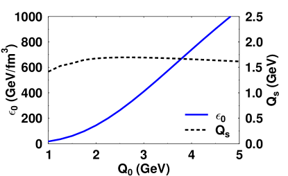
Fig. 1 shows our estimate for the inital energy density $\epsilon_{0}$ in the center of the collision as a function of the UV cutoff $Q_{0}$ for central collisions at RHIC using $\zeta^{2}=Q_{0}^{2}/(\alpha_{s}\sigma)$. We find that $Q_{s}$ only varies between 1.4 and 1.7 GeV if $Q_{0}$ is varied between 1 and 10 GeV. For a reasonable cutoff $Q_{0}=2.5$ GeV we have $\epsilon_{0}\approx 260$ GeV/fm³. This is compatible with a value of 130 GeV/fm³ at $\tau=0.1$ fm/$c$ found by T. Lappi in Lappi:06 . Note that $\epsilon_{0}$ only takes into account gluon modes with transverse momentum less than $Q_{0}$. Results for finite $\tau$ and the matching with hard processes to compute the total energy density and to eliminate the sensitivity to $Q_{0}$ will be discussed in a forthcoming publication FKLMB .

To conclude, we introduced a near-field expansion to solve the classical Yang-Mills equations for the collision of two large nuclei in the color glass picture. We found that strong longitudinal chromoelectric and magnetic fields dominate at early times. Using a coarse–graining of color charges we derived a simple expression for the initial energy density of the soft gluon field. A rough estimate implies values of about 260 GeV/fm³ at $\tau=0$ for the center of two colliding nuclei at RHIC.

We would like to thank B. Müller and S. A. Bass for discussions, and L. McLerran for his encouragement. We are grateful to S. Jeon, D. Kharzeev, T. Lappi and R. Venugopalan for helpful conversations. This work was supported by DOE grants DE-FG02-87ER40328, DE-AC02-98CH10886 and RIKEN BNL.

Figure 1: Initial energy density $\epsilon_{0}$ for $\tau\to 0$ and saturation scale $Q_{s}$ at RHIC as a function of the UV cutoff $Q_{0}$.