Properties of effective interactions and the excitation of 6^- states in ²⁸Si

Abstract

Cross-section and analyzing power data from $(p,p^{\prime})$ scattering to the $6^{-}$ states at 11.58 and 14.35 MeV in ²⁸Si, taken with energies of 80, 100, 134, and 180 MeV protons, have been analyzed using a distorted wave approximation with microscopically defined wave functions. The results, taken in conjunction with an analysis of an M6 electron scattering form factor, suggest that the two states exhaust respectively, $\sim 50$% and $\sim 60$% of the strengths of isoscalar and isovector particle-hole excitations from the ground state. The energy variation of data also suggests that the non-central components of the effective interactions at 80 and 100 MeV may need to be enhanced.

I Introduction

In a recent publication Amos et al. (2005), we demonstrated that analyses of complementary reaction data, from the scattering of electrons, of pions, and of protons leading to (dominantly isoscalar and isovector) $4^{-}$ states in ¹⁶O in the vicinity of 19 MeV excitation, could ascertain the degree of isospin and configuration mixing in the descriptions of those unnatural parity states. The existence of data from three distinct $4^{-}$ excitations in ¹⁶O bespoke of configuration mixing, given that a pure stretched scheme could only yield two such states. Those results also validated the tensor and spin-orbit character of the two-nucleon $NN$ effective interaction Amos et al. (2000) used in the distorted wave approximation (DWA) analyses of proton scattering (at 135 MeV) since those terms dominate scattering amplitudes of M4 transitions. Data were available from proton scattering (inelastic and charge exchange) and the characteristics (magnitude and shape of cross sections and spin observables as well as of form factors) clearly formed the conclusions drawn.

There are other nuclei with states that, in the simplest structure concept, are stretched particle-hole excitations from the ground. To our knowledge however, none have the variety of measured data as with the $4^{-}$ excitations in ¹⁶O. One such case is the excitation of $6^{-}$ states in ²⁸Si at 11.58 and 14.35 MeV above the ground. They are of interest to us first as proton scattering data exciting them have been measured for incident energies of 80, 100, 134, and 180 MeV and of both differential cross sections and analyzing powers Olmer et al. (1984). We consider this set of data herein in part to see if such suffice to identify configuration and/or isospin mixing within the actual states. The spectrum of ²⁸Si already infers that the particle-hole strength for excitation of the $6^{-}$ states could be fragmented. Pure stretched states formed just by promotion of a $0d_{\frac{5}{2}}$ particle into the $0f_{\frac{7}{2}}$ orbit, would result in just two transitions; the isoscalar and isovector combinations of the proton and neutron excitations. But, in the excitation energy range from 11 to 15 MeV, there are five known levels of that spin-parity Endt (1998).

Added interest lies in the fact that Skyrme-Hartree-Fock (SHF) calculations of the ground state of ²⁸Si have been made recently Richter and Brown (2003) with the resulting wave functions giving form factors in good agreement with available data from electron scattering. Two forms of the Skyrme interaction were used, of which we consider only the SHF wave functions determined using the so-called SkX_csb interaction Brown et al. (2000). The SkX_csb Hamiltonian is based on the SkX Hamiltonian Brown (1998) with a charge-symmetry-breaking (CSB) interaction added to account for nuclear displacement energies. Generally, with this SHF method, good agreement between theory and experiment has been achieved in extensive comparisons of measured nuclear charge-density distributions with calculated values for $p$-shell, $sd$-shell, and $pf$-shell nuclei and also with some selected magic and semi-magic nuclei up to ²⁰⁸Pb. They have been used more recently Amos et al. (2006) in analyses of total reaction cross sections of protons by which a new test of the neutron matter distribution was shown to be feasible. While much success has been had using the SHF densities and wave functions generated using the SkX_csb model, the canonical wave functions may not have a desirable long range character. So we have also used Woods-Saxon (WS) single nucleon bound state wave functions in place of them for comparison of scattering results.

Finally, as data have been taken at a set of energies, and as such unnatural parity transitions are dominated by the non-central components of the transition operator Amos et al. (2005), these observables may probe the tensorial character of the effective $NN$ interactions sensitively. That is so as the (complex) effective $NN$ interactions Amos et al. (2000) are energy as well as density dependent. Furthermore, the energy region is one for which past $g$-folding studies Amos et al. (2000) have successfully predicted elastic scattering observables. It is also one for which DWA calculations, made using the distorted wave functions from those $g$-folding optical potentials with the effective $NN$ $g$-matrix as the transition operator, gave good predictions of inelastic scattering observables to states of nuclei for which the spectroscopy was well determined Amos et al. (2000). An example is of excitation of the $2^{+}_{1}$ (4.43) MeV excitation in ¹²C when described by a complete $(0+2)\hbar\omega$ shell model study. But those successes, primarily, are measures of the central force components of the effective $NN$ interactions.

In the following section we describe the structure model for ²⁸Si and discuss the excitations to the 6^- states. That structure is tested by comparing predictions of the transverse magnetic form factor with data from electron scattering. Then, in Sec. III, we present relevant details of the DWA excitation matrix elements. The results of our DWA calculations are presented thereafter in Sec. IV and conclusions are given in Sec. V.

II The structure models

As noted above, we have used SHF and WS wave functions to describe the nucleon orbits in ²⁸Si. The SHF calculation Richter and Brown (2003) considered was that built with the SkX_csb interaction. Consequently proton and neutron densities differ slightly; how much being shown below in Fig. 1. In those studies, the single-particle occupancies $n_{j}$ were constrained to values obtained from shell-model calculations. That constraint resulted in a significantly improved agreement with most electron scattering form factors considered in Ref. Richter and Brown (2003). For ²⁸Si, these occupancies are listed for the dominant orbits in Table 1.

Table 1: The shell occupancies and binding energies taken for the ground state of ²⁸Si.

$\varphi_{j}$	Occupancy	B.E. (MeV)	$\varphi_{j}$	Occupancy	B.E. (MeV)
$0s_{\frac{1}{2}}$	2.0	29.7	$0d_{\frac{5}{2}}$	4.623	2.51
$0p_{\frac{3}{2}}$	4.0	16.1	$1s_{\frac{1}{2}}$	0.704	0.7
$0p_{\frac{1}{2}}$	2.0	12.4	$0d_{\frac{3}{2}}$	0.673	0.5

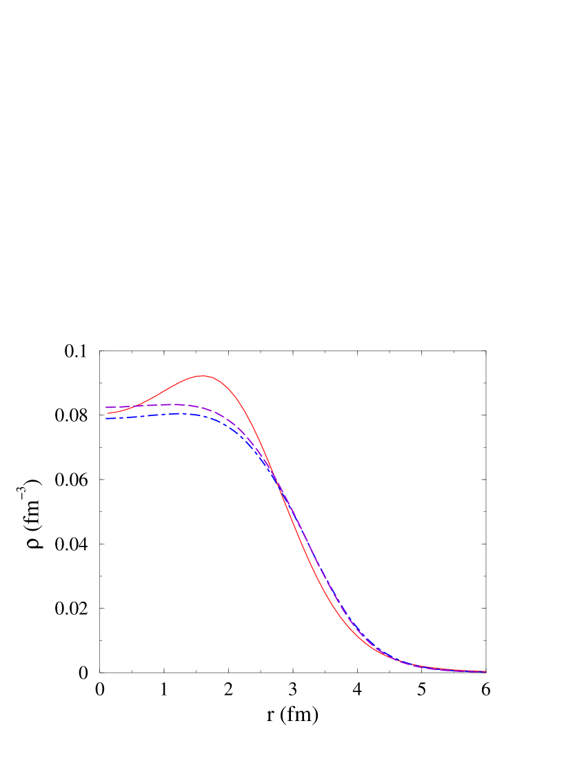
Figure 1: (Color online) The SHF model densities, proton (dot-dashed curve) and neutron (dashed curve) for ²⁸Si are compared to that found using WS wave functions but with the same shell occupancies. The proton and neutron WS distributions are identical with form displayed by the solid curve.

The binding energies listed in Table 1 were used with a Woods-Saxon bound state potential (radius $r_{0}=1.2$ fm, diffuseness $a=0.6$ fm) to define the WS bound state functions which form an alternative set to those given by the SHF calculation.

The SHF model densities (proton and neutron) are compared in Fig. 1 to the WS proton (neutron) density of the ground state of ²⁸Si. The difference between the SHF (proton and neutron) matter densities and the WS one with its surface peak are evident. The surface peaking behavior of the WS distribution tends more like that Richter and Brown Richter and Brown (2003) extracted from the electron form factor than does their SHF result.

II.1 One-body density matrix elements

One-body density matrix elements (OBDME) are required both in forming the optical potentials, with which we predict elastic scattering observables, and in the DWA amplitudes with which we predict inelastic and charge exchange observables. With a particle-hole matrix element cast in irreducible tensor form by

$$\left\langle\Psi_{J_{f}M_{f}}\left|a^{\dagger}_{j_{2}m_{2}}\ a_{j_{1}m_{1}}\right|\Psi_{J_{i}M_{i}}\right\rangle=$$

$$\hskip 28.45274pt\sum_{I(N)}(-1)^{(j_{1}-m_{1})}\left\langle j_{1}\,j_{2}\,m_{1}\,-m_{2}\left.\right|I\,-N\right\rangle\ \left\langle\Psi_{J_{f}M_{f}}\left|\left[a^{\dagger}_{j_{2}}\otimes{\tilde{a}}_{j_{1}}\right]^{IN}\right|\Psi_{J_{i}M_{i}}\right\rangle\ ,$$ (1)

use of the Wigner–Eckart theorem gives

$$\left\langle\Psi_{J_{f}M_{f}}\left|a^{\dagger}_{j_{2}m_{2}}\ a_{j_{1}m_{1}}\right|\Psi_{J_{i}M_{i}}\right\rangle=$$

$$\hskip 28.45274pt\sum_{I(N)}(-1)^{(j_{1}-m_{1})}\left\langle j_{1}\,j_{2}\,m_{1}\,-m_{2}\left.\right|I\,-N\right\rangle\times\frac{1}{\sqrt{2J_{f}+1}}\left.\left\langle J_{i}\,I\,M_{i}\,N\right|J_{f}\,M_{f}\right\rangle\ S_{j_{1}j_{2}I}\ ,$$ (2)

where the OBDME is

$$S_{j_{1}j_{2}I}=\left\langle\Psi_{J_{f}M_{f}}\left|\left|\left[a_{j_{2}}^{\dagger}\otimes{\tilde{a}}_{j_{1}}\right]^{I}\right|\right|\Psi_{J_{i}M_{i}}\right\rangle\ .$$ (3)

For elastic scattering from ²⁸Si (a spin-zero target), the OBDME are the ground state expectations of the particle-hole operator for zero angular momentum transfer ($I=0$). Often those numbers reduce simply to being the fractional shell occupancies of nucleons in the ground state $\sigma_{j}=n_{j}/(2j+1)$.

For the excitation of the stretched $6^{-};T$ states, transition OBDME for $I=6$ are required and similar to the development Amos et al. (2005) for the stretched $4^{-};T$ states in ¹⁶O, in the case of ²⁸Si, with states given by

$$\left|6^{-};T\right\rangle=\left|\left(d^{-1}_{\frac{5}{2}}f_{\frac{7}{2}}\right)6^{-};T\right\rangle=\frac{1}{\sqrt{\left[\left(1-\sigma_{\frac{7}{2}}\right)\sigma_{\frac{5}{2}}\right]}}\ \left[a^{\dagger}_{\frac{7}{2},\frac{1}{2}}\otimes{\tilde{a}}_{\frac{5}{2},\frac{1}{2}}\right]^{6,T}_{M_{6},M_{T}=0}\left|0^{+};0\right\rangle\ ,$$ (4)

where $\sigma_{j}$ is the fractional occupancy of protons (and of neutrons) in the shell $j$ in the ground state (listed in Table 1), the OBDME are

$$S_{\frac{5}{2}\frac{7}{2}6}(x)=\sqrt{\frac{13}{2}}\left\{\delta_{T,0}+\delta_{T,1}(-1)^{\left(1/2-x\right)}\right\}\sqrt{\left[\left(1-\sigma_{\frac{7}{2}}\right)\sigma_{\frac{5}{2}}\right]}\ ,$$ (5)

when $x=\pm\frac{1}{2}$ for a neutron and a proton respectively. With the shell occupancies listed in Table 1, the OBDME for excitation of stretched $6^{-}$ states has the magnitude of 2.238.

II.2 Electron scattering and the M6 transverse form factor

Electron scattering exciting the isovector $6^{-}$ state at 14.35 MeV has been measured Yen et al. (1980) and the M6 form factor extracted in the range of momentum transfer from 1 to nearly 3 fm^-1. That form factor was extracted from cross section data at two scattering angles using the plane wave definition,

$$\frac{d\sigma}{d\Omega}=4\pi\sigma_{M}R\left[F_{C\lambda}^{2}(q)+\left\{\frac{1}{2}+\tan^{2}(\theta/2)\right\}F_{T\lambda}^{2}(q)\right]\ .$$ (6)

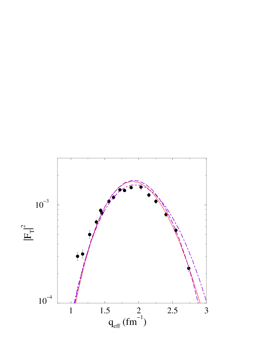
Figure 2: (Color online) The M6 transverse form factors calculated using oscillator (dashed curve), SHF model (solid curve), and WS (dot-dashed curve) wave functions compared with data Yen et al. (1980).

Excitation of the $6^{-};T=1$ state yielded $\left|F_{T}\right|^{2}=F_{T6}^{2}(q)$. The other factors in Eq. (6) are the Mott scattering cross section $\sigma_{M}$ and a recoil factor $R$ Yen et al. (1983). The M6 form factor is shown in Fig. 2 where it is plotted against an effective momentum transfer $q_{\text{eff}}$, to take into account the effect of acceleration of the electron by the Coulomb field of the target Yen et al. (1983). In this figure, the data are compared with three calculated results. That depicted by the dashed curve was found using $0\hbar\omega$ shell model (oscillator length $b=1.74$ fm) wave functions while that depicted by the solid curve was obtained using the SHF wave functions. The third, dot-dashed, curve is the result found by using WS wave functions. All calculated results determined by using the pure particle-hole description of the excited state (with shell occupancies given in Table 1, and so the spectroscopic amplitude of 2.238) have been scaled by 0.36. The results suggest that the strength of this particle-hole state is dissipated among others, with the 14.35 MeV state accounting for $\sim$60%.

III Elements of the DWA calculations

Cross sections for inelastic proton scattering exciting the $6^{-}$ states in ²⁸Si have been evaluated using a fully microscopic DWA theory of the processes Amos et al. (2000). As all details have been given in that review, only salient features are dealt with in this section. The distorted waves are generated from optical potentials formed by folding an effective in-medium $NN$ interaction with the OBDME of the target states. At each energy, the effective $NN$ interaction is generated from a mapping to solutions of Brueckner-Bethe-Goldstone equations (the $NN$ $g$ matrices). In coordinate space that effective $NN$ interaction is a mix of central, two-body spin-orbit and tensor forces all having form factors that are sums of Yukawa functions. Then with the Pauli principle taken into account, optical potentials from the folding are complex, nonlocal, and energy dependent. Such are formed and used in the DWBA98 program Raynal (1998) to predict elastic scattering observables. That same program finds distorted wave functions from those potentials for use in DWA calculations of the inelastic scattering cross sections and spin observables. The transition amplitudes for nucleon inelastic scattering from a nuclear target have the form Amos et al. (2000)

$${\cal T} = T^{M_{f}M_{i}\nu^{\prime}\nu}_{J_{f}J_{i}}(\Omega_{sc})$$ (7)

$$= \left\langle\chi^{(-)}_{\nu^{\prime}}({\bf k}_{o}0)\right|\left\langle\Psi_{J_{f}M_{f}}(1\cdots A)\right|\;A{\bf g}_{\text{eff}}(0,1)\;{\cal A}_{01}\left\{\left|\chi^{(+)}_{\nu}({\bf k}_{i}0)\right\rangle\right.\left.\left|\Psi_{J_{i}M_{i}}(1\cdots A)\right\rangle\right\}\ ,$$

where $\Omega_{sc}$ is the scattering angle and ${\cal A}_{01}$ is the antisymmetrization operator. The nuclear transition is from a state $|J_{i}M_{i}\rangle$ to a state $|J_{f}M_{f}\rangle$ and the projectile has spin projections $\nu$ and $\nu^{\prime}$ before and after the collision with the incoming and outgoing distorted waves being $\chi^{\pm}$. The incoming and outgoing relative momenta are ${\bf k}_{i}$ and ${\bf k}_{o}$ respectively. Then a cofactor expansion of the target states,

$$\left|\Psi_{JM}(1\cdots A)\right\rangle=\frac{1}{\sqrt{A}}\sum_{j,m}\left|\varphi_{jm}(1)\right\rangle\,a_{jm}(1)\,\left|\Psi_{JM}(1\cdots A)\right\rangle\ ,$$ (8)

allows expansion of the scattering amplitudes in the form of weighted two-nucleon elements since the terms $a_{jm}(1)\,\left|\Psi_{JM}(1\cdots A)\right\rangle$ in Eq. (8) are independent of coordinate ‘1’. Thus

$${\cal T} = \sum_{j_{1},j_{2}}\left\langle\Psi_{J_{f}M_{f}}(1\cdots A)\right|a^{\dagger}_{j_{2}m_{2}}(1)a_{j_{1}m_{1}}(1)\left|\Psi_{J_{i}M_{i}}(1\cdots A)\right\rangle$$ (9)

$$\hskip 28.45274pt\times\left\langle\chi^{(-)}_{\nu^{\prime}}({\bf k}_{o}0)\right|\left\langle\varphi_{j_{2}m_{2}}(1)\right|\ {\bf g}_{\text{eff}}(0,1)\ {\cal A}_{01}\left\{\left|\chi^{(+)}_{\nu}({\bf k}_{i}0)\right\rangle\ \left|\varphi_{j_{1}m_{1}}(1)\right\rangle\right\}$$

$$= \sum_{j_{1},j_{2},m_{1},m_{2},I(N)}(-1)^{(j_{1}-m_{1})}\frac{1}{\sqrt{2J_{f}+1}}\,\left<J_{i}\,I\,M_{i}\,N|J_{f}\,M_{f}\right>\left<j_{1}\,j_{2}\,m_{1}\,-m_{2}|I\,-N\right>\,S_{j_{1}\,j_{2}\,I}^{(J_{i}\to J_{f})}\$$

$$\hskip 56.9055pt\times\Bigl{<}\chi^{(-)}_{\nu^{\prime}}({\bf k}_{o}0)\Bigr{|}\left\langle\varphi_{j_{2}m_{2}}(1)\right|\ {\bf g}_{\text{eff}}(0,1)\ {\cal A}_{01}\left\{\left|\chi^{(+)}_{\nu}({\bf k}_{i}0)\right\rangle\ \left|\varphi_{j_{1}m_{1}}(1)\right\rangle\right\}\ ,$$

where reduction of the structure factor to OBDME for angular momentum transfer values $I$ follows that developed earlier Amos et al. (2005).

The effective interactions $g_{\text{eff}}(0,1)$ used in the folding to get the optical potentials have also been used as the transition operators effecting the excitations (of the $6^{-}$ states). As with the generation of the elastic scattering optical potentials from which the distorted waves are generated, antisymmetry of the projectile with the individual bound nucleons is treated exactly. The associated knock-out (exchange) amplitudes contribute importantly to the scattering cross section, both in magnitude and shape Amos et al. (2000). The OBDME and single particle wave functions required in these matrix elements are those specified in the previous section.

IV Results

IV.1 Elastic scattering of protons from ²⁸Si

The cross sections for the elastic scattering of 80, 100, 134, and 180 MeV protons from ²⁸Si calculated using the $g$-folding model for the relevant optical potentials are compared with data Olmer et al. (1984) in Fig. 3. Two potentials for each energy were formed, one set by folding the effective $NN$ interactions with the SHF wave functions and the other by using WS single particle wave functions. In all cases, the orbit occupancies were those specified previously in Table 1.

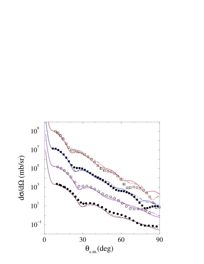
Figure 3: (Color online) $g$-folding model predictions of cross sections for the elastic scattering of 80, 100, 134, and 180 MeV protons from ²⁸Si compared with data. The predictions found by using the SHF structure are shown by the solid curves while those obtained with the WS single particle wave functions are displayed by the dash-dot curves.

The 80 MeV data and results are unscaled and are the lowest shown in the figure. For clarity, the other three results (and data) have been multiplied by 10², 10⁴, and 10⁶ for the 100, 134, and 180 MeV cases respectively. Our results, while good in comparison with the data, are not as perfect fits as has been found Olmer et al. (1984). But that study Olmer et al. (1984) used a phenomenological potential whose parameter values were determined by numerical inversion of data. In contrast, our results are predictions resulting from the use of model structures folded over effective interactions and with no a posteriori adjustments of any kind. The solid curves in this figure are the results obtained using the SHF model of structure while the dot-dashed curves are those obtained when WS bound state wave functions are used in place of the canonical ones of the SHF. The comparisons with data are quite good for cross section values larger than $\sim 10^{-1}$ mb/sr with the SHF predictions being preferable in general. Nevertheless there are some disagreements between the calculated and the experimental cross sections which, in view of the variations found between the SHF and the WS cross sections, bespeaks of a needed improvement in the details of the structure model. Particularly it is the mismatch to data having small values at larger scattering angles (and so larger momentum transfer values) that needs addressing in future. These disparities indicate that the structure of the densities inside the nucleus are most likely to blame.

That is emphasized in the comparison between our predictions and the associated analyzing power data Olmer et al. (1984). The elastic scattering analyzing power data and $g$-folding model predictions for the four energies considered are displayed in Fig. 4. The notation is the same as used in Fig. 3 with the 80 MeV results shown in the top left panel, the 100 MeV results placed in the top right panel and the 134 and 180 MeV results presented in the bottom, left and right panels, respectively.

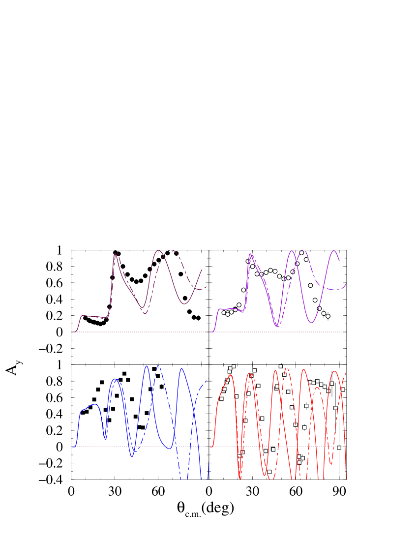
Figure 4: (Color online) $g$-folding model predictions of analyzing powers for the elastic scattering of 80, 100, 134, and 180 MeV protons from ²⁸Si compared with data. The notation is as used in Fig. 3.

There is obvious mismatch between predictions and data of this quantity. Also there is greater variation between the predictions made with the SHF structure and those made with the WS functions. Nonetheless the general trend of the data is found, more so with the 134 and 180 MeV results. Again we note that the phenomenological approach does far better in fitting than this but it must be remembered that in the phenomenological process, parameter adjustments are designed to yield best fits. That is so even if any data may be suspect. When using phenomenology, some independent condition or conditions (besides a fit to data) should be applied in defining a ‘good’ phenomenological potential. The analyzing power results are much more sensitive to the nature of the single particle bound state wave functions used to form the $g$-folding potentials. This was noted also in the review Amos et al. (2000) for many target masses, and at energies of 65 and 200 MeV notably. We have found smooth variations in these observables from 80 to 180 MeV; much smoother than the existent data in fact. However, all we may claim at this stage is that improved wave functions with which better fits to the cross section data need be found before more concrete statements resulting from the comparisons of analyzing powers can be made.

IV.2 Inelastic proton scattering to $6^{-}$ states of pure isospin

Cross sections for the excitation of an isoscalar 6^- state in ²⁸Si at 11.58 MeV excitation resulting from DWA calculations are displayed in Fig. 5. The structure used in those calculations was that of a pure particle-hole excitation as detailed above based upon the SHF ground state.

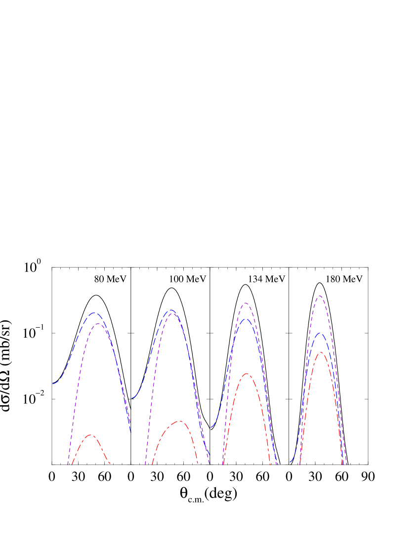
Figure 5: (Color online) DWA cross sections for the inelastic scattering of 80, 100, 134, and 180 MeV protons from ²⁸Si exciting a 6^- (T=0) state. In each panel the solid curves are the full calculated results, the long dashed curves depict those generated by purely the two-body tensor force as the transition operator, the small dashed curves are those generated by the two-body spin-orbit force alone, and the dot-dashed curves depict those cross sections generated using purely the central force components.

Therein, as in the ensuing figures, the results for 80, 100, 134, and 180 MeV are displayed in panels from left to right (as indicated). The full result (solid curve) is compared to those found when each of the three components of the effective transition operator are used by themselves, namely the central (dot-dash curve), the two-body spin-orbit $\mathbf{L}\cdot\mathbf{S}$ (dash curve), and the two-body tensor $\mathbf{S}_{12}$ (long dash curve) components. For this pure isoscalar transition, the central force component of the transition operator contributes only in a minor way gradually being more influential with increasing energy. In contrast, the contribution from the tensor force is substantial but slowly decreases with increasing energy. The two-body spin-orbit contributions are also substantial and increase to be the dominant feature of the scattering at 180 MeV. The results and the relative contributions are similar to those found previously Olmer et al. (1984) with the Love-Franey effective interaction. However, not only were those calculations Olmer et al. (1984) made using a distorted wave impulse approximation (DWIA) and hence did not evaluate explicit exchange matrix elements due to the Pauli principle, but also the Love-Franey force was one formed under a constraint to fit a set of free $NN$ scattering data and did not allow for medium modifications. Additionally, those older calculations also used phenomenological, local, optical potentials to generate the distorted waves with the parameters of those potentials chosen to find good fits to elastic scattering data. But that only requires specification of a suitable set of phase shifts and they are determined from the asymptotic forms of the distorted waves. The credibility of the distorted wave functions through the volume of the nucleus, properties needed in evaluation of inelastic scattering amplitudes, cannot be ascertained.

In Fig. 6 we show the cross sections obtained from DWA calculations of inelastic proton scattering at four energies and exciting a 6^- (T = 1) state at 14.35 MeV. The notation is as used in Fig. 5.

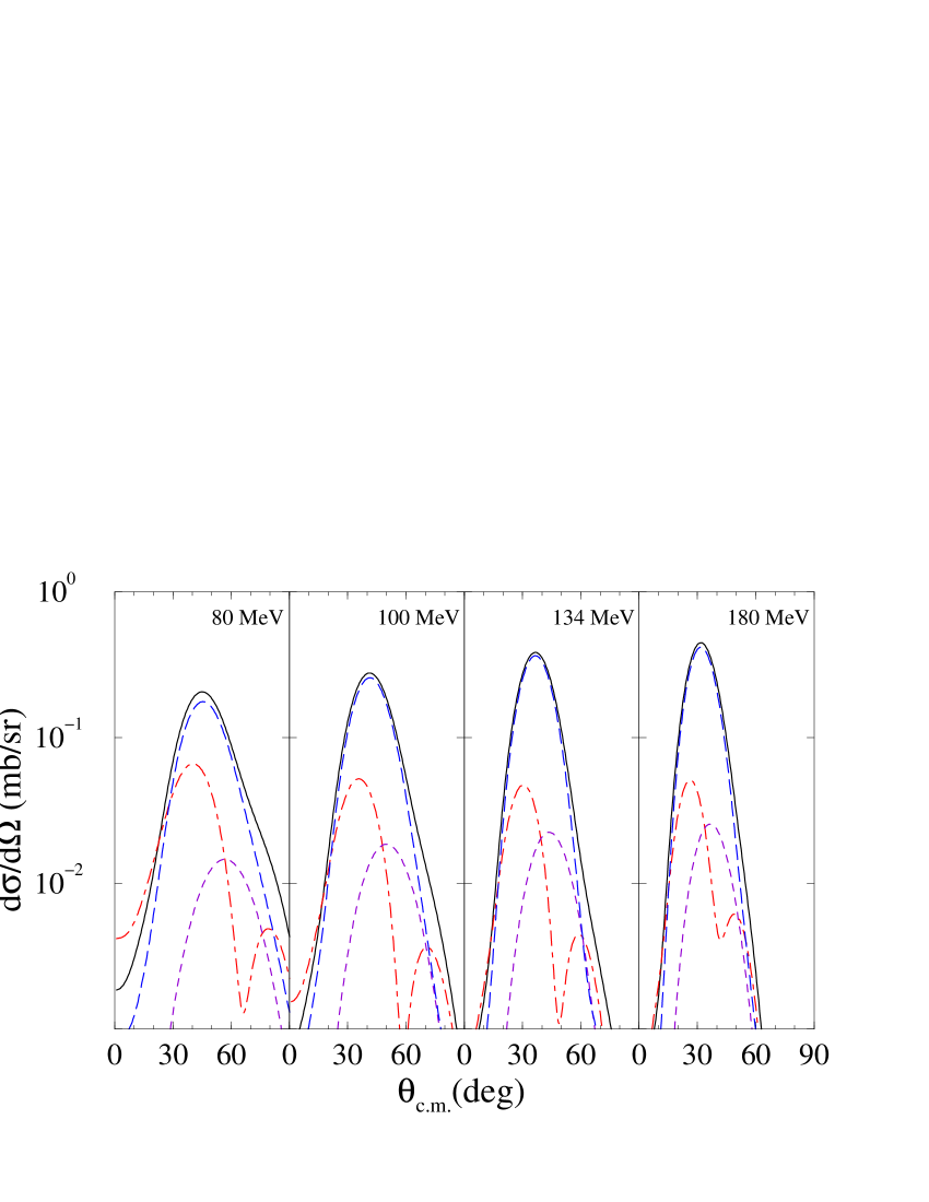
Figure 6: (Color online) DWA cross sections for the inelastic scattering of 80, 100, 134, and 180 MeV protons from ²⁸Si exciting a 6^- (T=1) state. The notation is as used in Fig. 5.

For this pure isovector transition, the tensor force is the dominant contributing component of the transition operator. It increases in magnitude with increasing energy so that at all four energies, the contributions from the central and two-body spin-orbit components remain minor. However they have distinctively different cross section component shapes with the effect of the central force being evident in the total result at forward angles and at 80 MeV.

Fig. 7 displays the cross sections from the excitation of the 11.58 MeV state treated as a pure isoscalar transition. The cross sections found by using the SHF wave functions and the OBDME for the simple particle-hole description of the excited state are depicted by the dashed curves. At all incident energies, the data are overestimated by those results. The solid curves then are those same cross sections multiplied by a factor of 0.26. For comparison, the cross sections found by using the WS wave functions, and with a similar scale reduction, are depicted by the dot-dashed curves. The choice of wave functions does not make significant change in the cross section results. The shapes and magnitudes of the 134 and 180 MeV data are quite well reproduced by these scaled, pure isoscalar, calculated cross sections. The 100 MeV scaled cross section replicates the overall magnitude and the large angle data reasonably but there is a distinct disparity between result and data at the forward scattering angles. Those disparities are even more evident in the 80 MeV results. Such were the case also in the previous analyses Olmer et al. (1984).

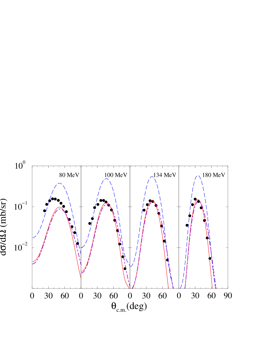
Figure 7: (Color online) Cross sections for the inelastic scattering of 80, 100, 134, and 180 MeV protons from ²⁸Si exciting a 6^- (T=0) state compared with data Olmer et al. (1984).

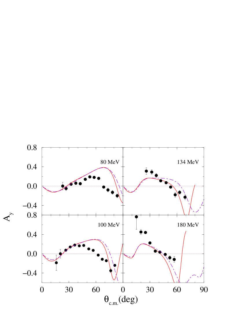
Figure 8: (Color online) Analyzing powers for the inelastic scattering of 80, 100, 134, and 180 MeV protons from ²⁸Si exciting a 6^- (T=0) state compared with data Olmer et al. (1984).

The analyzing powers from this isoscalar transition are depicted in Fig. 8 with the SHF and WS results again being displayed by the solid and dot-dashed curves respectively. The agreement between our calculated results and the data is only average in quality, but the trend of the data is replicated. As energy increases,, the positive peak in the data moves to smaller scattering angles and the data give negative values at the larger scattering angles. So also do our calculated results. In this observable the choice of wave functions (SHF or WS) has a slightly more noticeable effect than with the cross sections, particularly at large angles for the higher energies.

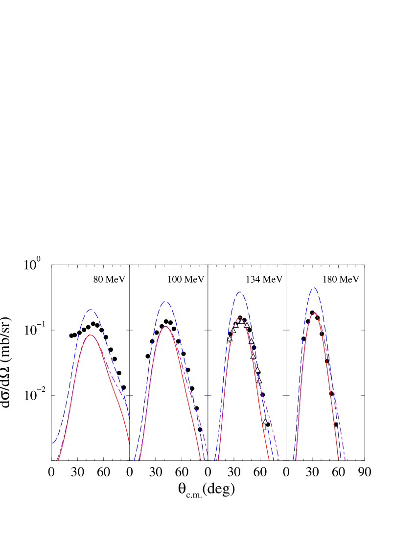
Figure 9: (Color online) Cross sections for the inelastic scattering of 80, 100, 134, and 180 MeV protons from ²⁸Si exciting a 6^- (T=1) state compared with data Olmer et al. (1984). The 134 MeV ($p,n$) data Fazely et al. (1985) ($\times\frac{1}{2}$) exciting the analogue state in ²⁸P are shown by the open triangles. The full calculation results are displayed by the dashed curves while the solid curves result when a scale of 0.41 is applied.

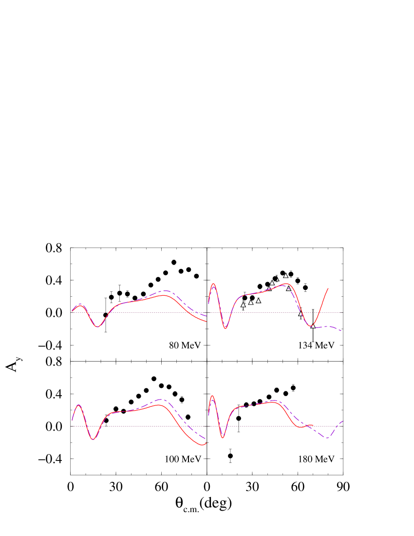
Figure 10: (Color online) Analyzing powers for the inelastic scattering of 80, 100, 134, and 180 MeV protons from ²⁸Si exciting a 6^- (T=1) state compared with data Olmer et al. (1984). The 134 MeV ($p,n$) data Fazely et al. (1985) exciting the analogue state in ²⁸P are shown by the open triangles. The solid curves depict the results found using the SHF wave functions while the dot-dashed curves are those found using the WS functions.

In Fig. 9 cross-section data Olmer et al. (1984) from inelastic proton scattering to the 14.35 MeV state of ²⁸Si are compared with our DWA results considering the transition to be purely isovector. In this case the solid curves depict results found using a scale factor of 0.41 on the total cross sections. While a slightly smaller value (0.36) was required to match the electron scattering form factor, the results are sufficiently similar to consider that the two data sets confirm the degree of configuration mixing in the isovector $6^{-}$ state. Again the results obtained by using the WS instead of the SHF wave functions are depicted by the dot-dashed curves. For this 14.35 MeV excitation, we note that the comparisons between data and calculated results are very similar to those found with the isoscalar transition. However, the disparities seen with energies of 80 and 100 MeV are accentuated while the 134 and 180 MeV results are somewhat in better agreement with data. In this figure we also include the cross sections measured at 134 MeV Fazely et al. (1985) from the charge exchange ($p,n$) reaction to the analogue $6^{-}$ state in ²⁸P. The actual data has been halved in accord with the isospin weighting coefficient that relates the ($p,n$) scattering to the ($p,p^{\prime}$) scattering to the $6^{-};T=1$ analogue state in ²⁸Si. The ($p,n$) data ($\times\frac{1}{2}$) are portrayed by the open triangles. That the two cross sections agree so well confirms the analogue character of the states involved and also argues for purity in isospin.

The analyzing powers associated with the cross sections discussed immediately above, are compared with data in Fig 10. Again there are some mismatching to the 80 and 100 MeV data though the trend as the incident energy increases is reflected by the calculated results. Now, however, the 134 and 180 MeV data are quite well reproduced, especially when one considers the ($p,n$) reaction values at 134 MeV.

We have made numerous evaluations also allowing degrees of isospin mixing in the two states for which there are data. That such could occur follows from the strong indication we found Amos et al. (2005) for such a mixing in the $4^{-}$ states in the spectrum of ¹⁶O. In this case though the two $6^{-}$ states to which there are scattering data lie $\sim 3$ MeV apart, there are a number of other $6^{-}$ states around and between them. However, no improvement in the shape of cross sections compared to the data results for any reasonable admixing of isospin, nor is there any significant improvement in the peak magnitude variation with energy.

V Conclusions

We have analyzed proton scattering cross sections and analyzing powers from the scattering of protons at 80, 100, 134, and 180 MeV from ²⁸Si. Both elastic scattering data and those from the excitation of two $6^{-}$ states have been considered. Those states, thought to be stretched, single particle-hole excitations upon the ground state, are excited dominantly by the spin-orbit and tensor force terms in the effective $NN$ interaction that is considered as the transition operator.

The 134 and 180 MeV data, elastic and inelastic, cross sections and analyzing powers, are quite well reproduced by our predictions when some configuration mixing is allowed to fragment the particle-hole strength among other known $6^{-}$ states in ²⁸Si. The complementary analyses of the M6 electron scattering form factor and of the $(p,p^{\prime})$ observables at 134 and 180 MeV exciting the (isovector) 14.35 MeV state strongly indicate that this transition exhausts $\sim 60$% of the isovector particle-hole strength. There are no electron scattering data from excitation of the 11.58 MeV state from which to extract a form factor, but the analyses of the 134 and 180 MeV $(p,p^{\prime})$ cross sections suggest that this transition is isoscalar and exhausts $\sim 50$% of that particle-hole strength.

The data taken with 80 and 100 MeV protons is not as well reproduced, notably the elastic scattering analyzing powers and the peak magnitudes for the $6^{-}$ excitations found using the same scale required to match data at 134 and 180 MeV. We note that the shape of the elastic scattering data do not reflect the smooth trend with energy at large scattering angles given by our microscopic model calculations. With the inelastic scattering cross sections, the 80 MeV, and to a lesser extent the 100 MeV, data also are larger at forward scattering angles than our predictions. Of course, these inelastic excitations are particularly sensitive to the spin-orbit and/or the tensor character of the effective $NN$ interaction. While the results at 134 and 180 MeV, taken in conjunction with those for excitation of the $4^{-}$ states in ¹⁶O with 134 MeV protons Amos et al. (2005), do give credibility to the relevant components of the effective $NN$ interaction at those energies, on the basis of the data considered, the strengths of the tensor components at 80 and 100 MeV may be weak. Analyses of more data from scattering with proton energies at and below 100 MeV, and from other stretched state excitations, are needed to ascertain any such adjustment to the effective interaction.