Probing nuclear skins and halos with elastic electron scattering

Abstract

I investigate the elastic electron scattering off nuclei far from the stability line. The effects of the neutron and proton skins and halos on the differential cross sections are explored. Examples are given for the charge distribution in Sn isotopes and its relation to the neutron skin. The neutron halo in ¹¹Li and the proton halo in ⁸B are also investigated. Particular interest is paid to the inverse scattering problem and its dependence on the experimental precision. These studies are of particular interest for the upcoming electron ion colliders at the GSI and RIKEN facilities.

I Introduction

The use of radioactive nuclear beams produced by fragmentation in high-energy heavy-ion reactions lead to the discovery of halo nuclei, such as ¹¹Li, about 20 years ago Ta85 . Nowadays a huge number of $\beta$-unstable nuclei far from stability are being studied thanks to further technical improvements. Unstable nuclei far from stability are known to play an important role in nucleosynthesis. Detailed studies of the structure and their reactions will have unprecedented impact on astrophysics BHM02 .

The first experiments with unstable nuclear beams aimed at determining nuclear sizes by measuring the interaction cross section in high energy collisions Ta85 . Successive use of this technique has yielded nuclear size data over a wide range of isotopes. Other techniques, e.g. isotope-shift measurements, have allowed to extract the charge size. The growth of a neutron skin with the neutron number in several isotopes have been deduced from nuclear- and charge-size data OST01 .

The charge (nucleon) density distribution can also be determined by electron (hadron) scattering experiments. Among hadron scattering, proton elastic scattering at intermediate energies is a good tool to probe the nucleon density distributions, due to its larger mean-free path in the nuclear medium. But, undoubtedly, it is the electron scattering off nuclei that provides the most direct information about charge distribution, which is closely related to the spatial distribution of protons Hof61 .

A technical proposal for an electron-heavy-ion collider has been incorporated in the GSI/Germany physics program Haik05 . A similar program exists for the RIKEN/Japan facility using Self-Confining Radioactive Ion Targets (SCRITs) Sud01 . In both cases the main purpose is to study the structure of nuclei far from the stability line. The advantages of using electrons in the investigation of the nuclear structure are mainly related to the fact that the electron-nucleus interaction is relatively weak. For this reason multiple scattering effects are usually small and the scattering process is described in terms of perturbation theory. Since the reaction mechanism in perturbation theory is well under control the connection between the cross section and quantities such as charge distributions, transition densities, response functions etc., is well understood Hof56 .

Theoretically, the shape of the density distribution includes detailed information on the internal nuclear structure. In the independent particle shell model the density distribution is the squared sum of the single-particle wave functions. No measurement of either nucleon distribution or the charge distribution for short-lived radioactive nuclei has been made so far.

Under the impulse approximation, or plane wave Born approximation, the charge form factor can be determined from the differential cross section of elastic electron scattering. Since the charge distribution, $\rho_{ch}(r)$, is obtained from the charge form factor by a Fourier transformation, one can experimentally determine $\rho_{ch}(r)$ by differential cross-section measurements covering a wide range of momentum transfer $q$. This leads to information on the size and diffuseness when the charge form factor is measured at least up to the first maximum. To accomplish this with a reasonable measuring time of one week, a luminosity larger than 10²⁶ cm^-2s^-1 is required, for example for the ¹³²Sn isotope Haik05 .

On the theoretical side the difference between the proton and neutron distributions can be obtained in the framework of Hartree-Fock (HF) method (see for example HL98 ) or Hartree-Fock-Bogoliubov (HFB) method (see for example Miz00 ; Ant05 ). As a rule of thumb, a theoretical calculation of the nuclear density is considered good when it reproduces the data on elastic electron scattering. But some details of the theoretical densities might not be accessible in the experiments, due to poor resolution or limited experimental reach of the momentum transfer $q$. Recent works have also looked at electron scattering from halo nuclei, see e.g. refs. GMG99 ; Ers05 ; KA06 .

In this work I study the general features of elastic electron scattering off unstable nuclei. Here I focus on using the general features of what is theoretically known about skins and halos to look for their respective signatures in the data. Only a few specific and representative nuclear density cases are used. The paper is organized as follows. After a general introduction of elastic electron scattering in section 2, I show in section 3 how the telltales of neutron and proton skins and halos become visible in the differential cross sections for elastic electron scattering. Section 4 presents a study of the inverse scattering problem, which poses a challenge for extracting the charge density profiles from the experimental data. The conclusions are presented in section 5.

II Elastic Electron Scattering

In the plane wave Born approximation (PWBA) the relation between the charge density and the cross section is given by

$$\left(\frac{d\sigma}{d\Omega}\right)_{\mathrm{PWBA}}=\frac{\sigma_{M}}{1+\left(2E/M_{A}\right)\sin^{2}\left(\theta/2\right)}\ |F_{ch}\left(q\right)|^{2},$$ (1)

where $\sigma_{M}=(e^{4}/4E^{2})\cos^{2}\left(\theta/2\right)\sin^{-4}\left(\theta/2\right)$ is the Mott cross section, the term in the denominator is a recoil correction, $E$ is the electron total energy, $M_{A}$ is the mass of the nucleus and $\theta$ is the scattering angle.

The charge form factor $F_{ch}\left(q\right)$ for a spherical mass distribution is given by

$$F_{ch}\left(q\right)=4\pi\int_{0}^{\infty}dr\ r^{2}j_{0}\left(qr\right)\rho_{ch}\left(r\right),$$ (2)

where $q=2k\sin\left(\theta/2\right)$ is the momentum transfer, $\hbar k$ is the electron momentum, and $E=\sqrt{\hbar^{2}k^{2}c^{2}+m_{e}^{2}c^{4}}$. The low momentum expansion of eq. 2 yields the leading terms

$$F_{ch}\left(q\right)/Z=1-\frac{q^{2}}{6}\left\langle r_{ch}^{2}\right\rangle+\cdots.$$ (3)

Thus, a measurement at low momentum transfer yields a direct assessment of the mean square radius of the charge distribution, $\left\langle r_{ch}^{2}\right\rangle^{1/2}$. However, as more details of the charge distribution is probed more terms of this series are needed and, for a precise description of it, the form factor dependence for large momenta $q$ is needed.

A theoretical calculation of the charge density entering eq. 2 can be obtained in many ways. Let $\rho_{p}\left(\mathbf{r}\right)$ and $\rho_{n}\left(\mathbf{r}\right)$ denote the point distributions of the protons and the neutrons, respectively, as calculated, e.g. from single-particle wavefunctions obtained from an average one-body potential well, the latter in general being different for protons and neutrons. If $f_{Ep}\left(\mathbf{r}\right)$ and $f_{En}\left(\mathbf{r}\right)$ are the spatial charge distributions of the proton and the neutron in the non-relativistic limit, the charge distribution of the nucleus is given by

$$\rho_{ch}\left(\mathbf{r}\right)=\int\rho_{p}\left(\mathbf{r}^{\prime}\right)\ f_{Ep}\left(\mathbf{r-r}^{\prime}\right)\ d^{3}r^{\prime}+\int\rho_{n}\left(\mathbf{r}^{\prime}\right)\ f_{En}\left(\mathbf{r-r}^{\prime}\right)\ d^{3}r^{\prime}.$$ (4)

The second term on the right-hand side of eq. 4 plays an important role in the interpretation of the charge distribution of some nuclear isotopes. For example, the half-density charge radius increases 2% from ⁴⁰Ca to ⁴⁸Ca, whereas the surface thickness decreases by 10% with the result that there is more charge in the surface region of ⁴⁰Ca than of ⁴⁸Ca Fro68 . This also implies that the rms charge radius of ⁴⁸Ca is slightly smaller than that of ⁴⁰Ca. The reason for this anomaly is that the added $f_{7/2}$ neutrons contribute negatively to the charge distribution in the surface and more than compensate for the increase in the rms radius of the proton distribution.

For the proton the charge density $f_{Ep}\left(r\right)$ in eq. 4 is taken as an exponential function, corresponding to a form factor $\widetilde{f}_{Ep}\left(q\right)=(1+q^{2}/\Lambda^{2})^{-1}$ (see Appendix A). For the neutron a good parametrization is $\widetilde{f}_{En}(q)=-\mu_{n}\tau\widetilde{f}_{Ep}(q)/(1+p\tau)$, where $\mu_{n}$ is the neutron magnetic dipole moment and $\tau=q^{2}/4m_{N}$. We will use $\Lambda^{2}=0.71$ fm^-2 (corresponding to a proton rms radius of 0.87 fm) and $p=5.6$, which Galster et al. Gal71 have shown to reproduce electron-nucleon scattering data.

Eqs. 1-4 are based on the first Born approximation. They give good results for light nuclei (e.g. ¹²C) and high-energy electrons. For large-$Z$ nuclei the agreement with experiment is only of a qualitative nature. The effects of distortion of the electron waves have been studied by many authors (see, e.g. ref. MF48 ; Yenn53 ; Cut67 ). More important than the change in the normalization of the cross section is the displacement of the minima. It is well known that a simple modification can be included in the PWBA equation reproducing the shift of the minima to lower $q$’s. One replaces the momentum transfer $q$ in the form factor of eq. 1 with the effective momentum transfer $q_{eff}=q\left(1+3Ze^{2}/2R_{ch}E\right)$, where $E$ is the electron energy and $R_{ch}\simeq 1.2\ A^{1/3}$ fm. This is because a measurement at momentum transfer $q$ probes in fact  $|F(q)|^{2}$ at $q=q_{eff}$ due to the attraction the electrons feel by the positive charge of the nucleus. This expression for $q_{eff}$ assumes a homogeneous distribution of charge within a sphere of radius $R_{ch}$.

A realistic description of elastic electron scattering cross sections requires full solution of the Dirac equation. The Dirac equation for elastic scattering from a charge distribution can be found in standard textbooks, e.g. EG88 . Numerous DWBA codes based on Dirac distorted waves have been developed and are public. Since the inclusion of Coulomb distortion is straight-forward, we will concentrate on the information which can be extracted from elastic electron scattering, which is encoded in the form-factor of eq. 2. Later we will study the problem of extracting the full nuclear density from the form factor. For simplicity, we will also neglect the effect of the charge distribution of the neutron itself. This effect is particularly important for large $q$-transfers. For heavy nuclei it can change $\left|F_{ch}\left(q\right)\right|^{2}$ by 10-20% in the q-range of 1.5 - 2 fm^-1.

III Skins and Halos

III.1 Neutron Skins

Appreciable differences between neutron and proton radii are expected Dob96 to characterize nuclei at the border of the stability line. The liquid drop formula expresses the binding energy of a nucleus with $N$ neutrons and $Z$ protons as a sum of bulk, surface, symmetry and Coulomb energies ${E/A}=a_{V}A-a_{S}A^{2/3}-S(N-Z)^{2}/A-a_{C}Z^{2}/A^{1/3}\mp a_{p}A^{-1/2},$where $a_{V}$, $a_{S}$, $a_{p}$, $S$ and $a_{C}$ are parameters fitted to experimental data of binding energy of nuclei. This equation does not distinguish between surface ($S$) and volume ($V$) symmetry energies. As shown in ref. Da03 , this can be achieved by partitioning the particle asymmetry as $N-Z=N_{S}-Z_{S}+N_{V}-Z_{V}$. The total symmetry energy $S$  then takes on the form $S=S_{V}(N_{V}-Z_{V})^{2}/A+S_{S}(N_{S}-Z_{S})^{2}/A^{2/3}.$ Minimizing under fixed $N-Z$ leads to an improved liquid drop formula Da03 with the term $S(N-Z)^{2}/A$ replaced by

$$S_{V}{\frac{(N-Z)^{2}}{A[1+\left(S_{V}/S_{S}\right)A^{-1/3}]}}.$$ (5)

The same approach also yields a relation between the neutron skin $R_{np}=R_{n}-R_{p}$, and $S_{S}$, $S_{V}$, namely Da03

$$\frac{R_{n}-R_{p}}{R}=\frac{A}{6NZ}(N_{S}-Z_{S})=\frac{A}{6NZ}\frac{N-Z-\left(a_{C}/12S_{V}\right)ZA^{2/3}}{1+\left(S_{S}/S_{V}\right)A^{1/3}},$$ (6)

where $R=(R_{n}+R_{p})/2$, and $R_{n}$ ($R_{p}$) is the half-density neutron (proton) distribution radius.

Here the Coulomb contribution is essential; e.g. for $N=Z$  the neutron skin $R_{np}$ is negative due to the Coulomb repulsion of the protons. A wide variation of values of $S_{V}$ and $S_{S}$ can be found in the literature. These values have been obtained by comparing the above predictions for energy and neutron skin to theoretical calculations of nuclear densities and experimental data on other observables Da03 ; St05 . The values of $a_{C}=0.69$ MeV and $S_{V}=28$ MeV, which will be used here, are compatible with fits of the binding energy and symmetry energy of known nuclei St05 . Using these values and $R=1.2A^{1/3}$ fm, one gets, for large $A$ (with $A\gg 1$, $NZ\simeq A^{2}/4$),

$$R_{np}=R_{n}-R_{p}\simeq 0.8\left(\frac{S_{V}}{S_{S}}\right)\left(\delta-2.05\times 10^{-3}ZA^{-1/3}\right)\text{ fm},$$ (7)

where $\delta=\left(N-Z\right)/A$ is the asymmetry parameter. The ratio $S_{V}/S_{S}$ varies within the range $2\lesssim S_{S}/S_{V}\gtrsim 3$ by adjusting eq. 6 to the dependencies of skin sizes on asymmetry and on the neutron-proton separation-energy difference constraints St05 . If one assumes that the central densities for neutrons and protons are roughly the same and that they are both described by a uniform distribution with sharp-cutoff radii, $R_{n}$ and $R_{p}$, one finds $R_{np}\simeq 0.8A^{1/3}\delta$ fm. This shows that the sharp sphere model is too simple and that in this model the central densities for proton and neutrons have to differ if eq. 6 is to remain valid.

On the experimental front, a study of antiprotonic atoms published in reference Trz01 obtained the following fitted formula for the neutron skin of stable nuclei in terms of the root mean square (rms) radii of protons and neutrons

$$\Delta r_{np}=\left\langle r_{n}^{2}\right\rangle^{1/2}-\left\langle r_{p}^{2}\right\rangle^{1/2}=\left(-0.04\pm 0.03\right)+\left(1.01\pm 0.15\right)\delta\ \text{fm.}$$ (8)

The relation of the mean square radii with the half-density radii for a Fermi distribution is roughly given by $\left\langle r_{n}^{2}\right\rangle=3R_{n}^{2}/5+7\pi^{2}a_{n}^{2}/5$, where $a_{n}$ is the diffuseness parameter. For heavy nuclei, assuming $a_{n}=a_{p}\ll R_{n},R_{p}$, one gets approximately the same linear dependence on the asymmetry parameter as in eq. 7 (neglecting the small contribution of the $A^{-1/3}$ term).

In this work we will use eq. 8 as the starting point for accessing the dependence of electron scattering on the neutron skin of heavy nuclei. Applying it to calcium isotopes as an example, one obtains that the neutron skin varies from $-0.15$ fm for ³⁵Ca (proton-rich with negative neutron skin) to $0.25$ fm for ⁵³Ca. A negative neutron skin obviously means an excess of protons at the surface. For unstable nuclei no study as the one leading to eq. 8 is experimentally available. Nucleon knockout reactions with secondary unstable nuclear beams, and other techniques, have been used to determine the interaction radii of neutron rich nuclei Ta85 . These radii are thought to represent the extension of the neutron distribution. But very little is known about the charge distribution in neutron-rich nuclei.

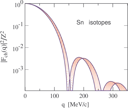
Figure 1: The charge form factor squared for elastic electron scattering off tin isotopes, as a function of the momentum transfer. The two curves are for the extreme values of the asymmetry parameter $\delta=(N-Z)/A$, that is $\delta=0$ ($N=Z=50$), and $\delta=4/9$ ($N=90$).  The curves form an envelope around other curves with intermediary values of $\delta$.

For heavy nuclei the charge and neutron distributions can be described by a Fermi distribution. The diffuseness is usually much smaller than the half-density radius, $a_{p,n}\ll R_{p,n}$. The neutron skin is then given by $R_{np}=R_{n}-R_{p}\simeq\sqrt{5/3}\ \Delta r_{np}$. We assume further that the nuclear charge radius is represented by $R_{p}=1.2A^{1/3}\ \mathrm{fm}-R_{np}/2$ with $\Delta r_{np}$ given by eq. 8. Figure 1 shows the charge form factor squared for elastic electron scattering off tin isotopes, as a function of the momentum transfer. The two solid curves are for the extreme values of the asymmetry parameter $\delta=(N-Z)/A$, that is $\delta=0$ ($N=Z=50$), and $\delta=4/9$ ($N=90$). The curves form an envelope around other curves with intermediary values of $\delta$. The first and second minima of the form factors occur at $q_{1}=4.49/R_{p}$ and $q_{2}=7.73/R_{p}$, respectively, corresponding to the zeroes of the transcendental equation $\tan\left(qR_{p}\right)=qR_{p}$.

Using the approximations discussed in the above paragraph, i.e. $R_{p}=1.2A^{1/3}\ \mathrm{fm}-R_{np}/2$ with $\Delta r_{np}$, $R_{np}=\Delta r_{np}$, and the experimental value given in eq. 8, we conclude that the linear dependence of $R_{p}$ with the neutron skin (and with the asymmetry parameter $\delta$), also implies a linear dependence of the position of the minima,

$$q_{1}\simeq\frac{3.74}{A^{1/3}}\ \ \left[1-0.535\frac{(N-Z)}{A^{4/3}}\right]^{-1}\ \mathrm{fm}^{-1},\ \ \ \ \ \ \ \ \mathrm{and}\ \ \ \ \ \ q_{2}=1.72\ q_{1}\ .$$ (9)

For ¹⁰⁰Sn the first minimum is expected to occur at $q_{1}=0.806$ $\mathrm{fm}^{-1}=159$ MeV/c, while for ¹³²Sn it occurs at $q_{1}=0.754$ $\mathrm{fm}^{-1}=149$ MeV/c.

Figure 2 shows the value of $q_{1}$ for calcium, tin and uranium isotopes, as a function of the asymmetry parameter $\delta$. The variation of $q_{1}$ with the neutron skin of neighboring isotopes, $\Delta q_{1}\simeq 2/A^{8/3}$ fm^-1, is too small to be measured accurately. The first minimum, $q_{1}$, changes from $220$ MeV/c for ³⁵Ca to $204$ MeV/c for ⁵³Ca, approximately 7%, which is certainly within the experimental resolution. Of course, sudden changes of the neutron skin with $\delta$ might happen due to shell closures, pairing, and other microscopic effects.

To be more specific, let us assume that a reasonable goal is to obtain accurate results for the charge radius $\left\langle r_{p}^{2}\right\rangle^{1/2},$ so that $\delta\left\langle r_{p}^{2}\right\rangle^{1/2}<0.05$ fm. This implies that the measurement of $q_{1}$ has to be such that $\left(\Delta q_{1}/q_{1}\right)<q_{1}\left[\text{fm}^{-1}\right]\%$, with $q_{1}$ in units of fm^-1 and the right-hand side of the inequality yielding the percent value. For ⁵³Ca, one has q${}_{1}=$ $1.11$ fm^-1, meaning that the experimental resolution on the value of $q_{1}$ has to be within 1% if $\delta\left\langle r_{p}^{2}\right\rangle^{1/2}<0.05$ fm is a required precision. The situation improves for heavier nuclei, as becomes evident from figure 2.

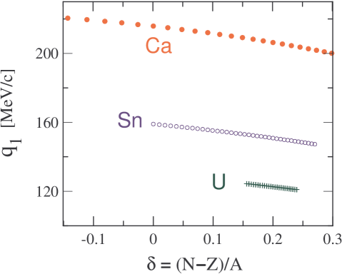
Figure 2: Position of the first minimum $q_{1}$ for elastic electron scattering off calcium, tin and uranium isotopes, as a function of the asymmetry parameter $\delta$.

The neutron skin dependence is also seen in the height of the second bump, after the first minimum. This bump occurs at $q_{m}\simeq 6/R_{p}$. For a Woods-saxon density this peak will be reduced compared to the first maximum by a factor $[g(q_{m}a)/12]^{2}$, where $g(q_{m}a)$ is a function of the diffuseness parameter $a$. $g$ is closely given by the Fourier transform of an Yukawa function, its value at $q_{m}a$ is of the order of $1/2$ and its variation around $q_{m}$ is weak, $g(qa)\sim 1/\left(1+q^{2}a^{2}\right)$ (see Appendix A). Thus, the dependence of the height of the second maximum upon the neutron skin is a less appropriate tool than the location of the first minimum. Of course, the ultimate test of a given theoretical model will be a good reproduction of the measured data, below and beyond the first minimum.

III.2 Neutron halos

For light halo nuclei composed of a core nucleus and an extended distribution of halo nucleons, the nuclear matter form factor can be fitted with the simple expression

$$F(q)/A=\left(1-g\right)\exp\left(-q^{2}a_{1}^{2}/4\right)+\frac{g}{1+a_{2}^{2}q^{2}},$$ (10)

where $g$ is the fraction of nucleons in the halo. In this expression the first term  follows from the assumption that the core is described by a Gaussian and the second term assumes that the halo nucleons are described by an Yukawa distribution (see Appendix A). Taking ¹¹Li as an example, the following set of parameters can be used $g=0.18,$ $a_{1}=2.0$ fm and $a_{2}=6.5$ fm. This means that $g=2/11$ nucleons are in the halo, the size of the core is roughly 2 fm, and the size of the halo is 6.5 fm. Although only few nucleons are in the halo they change dramatically the shape of the form factor, as shown in figure 3. The dashed-dotted curve is the squared charge form factor. The dotted curve applies for the matter density of the halo neutrons. When the core (dashed curve) and halo nucleon distributions are combined the squared form factor for the total matter distribution (solid curve) clearly displays the halo signature. Thus, even when the individual contribution of the halo nucleons is small and barely visible in a linear plot of the matter distribution, it is very important for the form factor of the total matter distribution. It is responsible for the narrow peak which develops at low momentum transfers. This signature of the halo was indeed the motivation for the early experiments with radioactive beams. The narrow peak was observed in momentum distributions following knockout reactions Ta85 .

Elastic electron scattering will not be sensitive to the narrow peak of $\left|F(q)\right|^{2}$ (matter distribution form factor) at small momentum $q$, but to the the charge distribution form factor, $\left|F_{ch}(q)\right|^{2},$ which in the case of ¹¹Li will be similar to the dashed-dotted curve in figure 3. The determination of this form factor will tell us if the core has been appreciably modified due to the presence of the halo nucleons. It is worthwhile mentioning that many of what we call core nuclei are also short-lived and very little is known about their charge distribution.

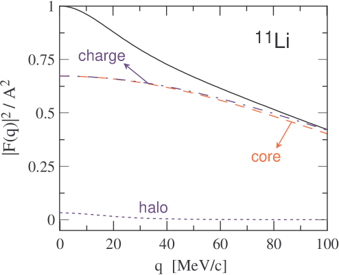
Figure 3: Form factor, $|F(q)|^{2}/A^{2}$, for ¹¹Li showing the individual contributions of the core and of the halo nucleons.  The dotted (halo), dashed (core) and solid (total) curves are form factors for the matter distribution. The dashed-dotted curve is the charge form factor, $|F_{ch}(q)|^{2}/Z^{2}$.

In order to explain the spin, parities, separation energies and size of exotic nuclei consistently a microscopic calculation is needed. One possibility is to resort to a Hartree-Fock (HF) calculation. Unfortunately, the HF theory cannot provide the predictions for the separation energies within the required accuracy of hundred keV. Here we use a simple and tractable HF method  BBS89 to generate synthetic data for the charge-distribution of ¹¹Li. Details of this method is described in ref. SB97 . Assuming spherical symmetry, the equation for the Skyrme interaction can be written as

$$\left[-\mathbf{\nabla}\frac{\hbar^{2}}{2m^{\ast}(r)}\mathbf{\nabla}+V(\mathbf{r})\right]\psi_{i}(\mathbf{r})=\epsilon_{i}\psi_{i}(\mathbf{r})$$ (11)

where $\,m^{\ast}(r)\,$ is the effective mass. The potential $\,V(\mathbf{r})\,$ has a central, a spin-orbit, and a Coulomb term

$$V(\mathbf{r})=V_{\mathrm{central}}+V_{\mathrm{spin-orbit}}+V_{\mathrm{Coulomb}}.$$ (12)

The central potential is multiplied by a constant factor $\,f\,$ only for the last neutron configuration:

$$V_{\mathrm{central}}(r)=fV_{HF}(r),\left\{\begin{array}[c]{l}f\neq 1\quad\mathrm{for\;last\;neutron\;configuration}\\ f=1\quad\mathrm{otherwise.}\end{array}\right.$$ (13)

Thus, the last neutron configuration (last orbits) is treated differently from the other orbits in the HF potential in order to reproduce the neutron separation energy of the neutron-rich nucleus. The factor  $f$  in Eq. 13 is arbitrary ($f=0.82$ for the last neutrons in ¹¹Li BBS89 ). It roughly scales with the inverse of the fraction of nucleons in the halo, and simulates a weaker potential at the halo region. This model was successful to explain most features of the light-neutron rich nuclei BBS89 ; Sa92 . It can also explain the magnitude of the nuclear sizes. In order to obtain the nuclear sizes, the rms radii of the occupied nucleon orbits are multiplied by the shell model occupation probabilities, which are also obtained in the calculations. The final radius is obtained by adding the core radius. It is important to notice that the physics of ¹¹Li is not treated very well because of the pairing interaction. This is needed to make ¹¹Li bound while ¹⁰Li is unbound. In this aspect, the model adopted here is only useful as a qualitative tool.

	$j_{\mathrm{halo}}$	$\sqrt{\langle r^{2}\rangle}_{\mathrm{cal}}\;$ (fm)	$\sqrt{\langle r^{2}\rangle}_{\exp}\;$ (fm)
9Li (core)		2.45	2.43 $\pm$ 0.07†
11Li	$1p_{1/2}$	5.36
	$2s_{1/2}$	7.61
SM		3.26	3.62 $\pm$ 0.19†
† from ref. Ege02 .

Table 1 - Single particle properties of ¹¹Li.  The second column gives the spins of the most probable occupied orbits. The third column is the result of HF calculations for the rms radii associated with these orbits, and the last column gives the rms radii of the matter distribution of these nuclei.

As the effective interaction, a parameter set of the density dependent Skyrme force, so called BKN interaction BKN , is adopted. The parameter set of BKN interaction has the effective mass m^∗/m =1 and gives realistic single particle energies near the Fermi surface in light nuclei. The original BKN force has no spin-orbit interaction. In the present calculations, I introduce the spin-orbit term in the interaction so that the single-particle energy of the last neutron orbit becomes close to the experimental separation energy. In this way, the asymptotic form of the loosely-bound wave function becomes realistic in the neutron-rich nucleus. The large r.m.s. radii of the valence neutron orbits is attributed to the small separation energy. The calculated value is enough to create the halo structure in the HF wave functions. In ¹¹Li, the last occupied orbits is taken to be 1p_1/2 and 2s_1/2.

We took the cut-off radius of H-F calculation to be $R=40\,\mbox{fm}$ which is necessary to include properly the loosely bound nature of the neutron wave function. The separation energy for the valence nucleons is S${}_{2n}(theo)=0.274$ MeV, which is to be compared with the experimental one S${}_{2n}(exp)=0.247\pm 0.080$ MeV TUNL . The column indicated by $\,j_{\mathrm{halo}}\,$ in Table 1 displays the most probably occupied orbits. The final radius is obtained by adding the core radius, and is given in the row indicated by SM.

The elastic form factor for the matter distribution obtained in the HF calculations are very close to the ones calculated by the empirical formula 10. In figure 3 we show the charge form factor, $\left|F_{ch}(q)\right|^{2},$ by a dashed-dotted line. There is very little difference from the simpler empirical parametrization of eq. 10. The lack of minima, and of secondary peaks (as in eq. 10), makes it difficult to extract from $\left|F_{ch}(q)\right|^{2}$ more detailed information on the charge-density profile. Parametrizations like eq. 10 which apparently lack of a sound physical basis are not particular to loosely bound nuclear systems. For example, in the case of ⁶Li a good fit to experimental data was obtained with Sue67

$$\left|F_{ch}(q)\right|^{2}\propto\exp(-a^{2}q^{2})-Cq^{2}\exp(-b^{2}q^{2}),$$

with $a=0.933$ fm, $b=1.3$ fm, and $C=0.205$. However, the data Sue67 cannot be fitted by using a model in which the nucleons move in a single-particle potential.

III.3 Proton Halos

Here I will consider ⁸B as a prototype of proton halo nucleus. This nucleus is perhaps the most likely candidate for having a proton halo structure, as its last proton has a binding energy of only 137 keV. The charge density for this nucleus can be calculated in the framework of the Skyrme HF model. We will use here the results obtained in ref. Shyam , where axially symmetric HF equations were used with SLy4 Chab97 Skyrme interaction which has been constructed by fitting the experimental data on radii and binding energies of symmetric and neutron-rich nuclei. Pairing correlations among nucleons have been treated within the BCS pairing method. The form factor squared for the charge density in ⁸B is shown in figure 4, normalized to mass number for matter distribution, and to charge number for charge distribution.

The width of the charge form factor squared corresponding to the plot in figure 4 is $\Delta_{ch}=0.505$ fm${}^{-1}=99.6$ MeV/c. The corresponding values for the form factors for neutron and total matter distributions are, respectively, $\Delta_{n}=0.512$ fm${}^{-1}=101$ MeV/c and $\Delta_{tot}=0.545$ fm${}^{-1}=108$ MeV/c. This amounts to an approximately 10% difference between matter and charge form factors in ⁸B.

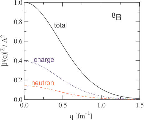
Figure 4: Form factor squared for ⁸B showing the contribution of neutron, $|F(q)|^{2}/N^{2}$, (dashed) charge, $|F(q)|^{2}/Z^{2}$, (dotted) and total, $|F(q)|^{2}/A^{2}$, (solid) matter distribution of nucleons.

The proton halo in ⁸B is mainly due to the unpaired proton in the p_3/2 orbit. It is clear that for such a narrow halo the size of the nucleon also matters. The relevance of the nucleon size is shown in figure 5 where a slice of the nucleon is included in a thin spherical shell of radius $r$ and thickness $dr$ from the center of the nucleus. If the position of the nucleon is given by $R$, the part of the proton charge included in the spherical shell is given by

$$d\rho_{ch}=2\pi r^{2}dr\int_{0}^{\pi}d\theta\ \rho_{p}\left(\mathbf{x}\right)\sin\theta,$$ (14)

where $\rho_{p}\left(\mathbf{x}\right)$ is the charge distribution inside a proton at a distance $\mathbf{x}$ from its center. The coordinates are shown in figure 5. They are related by $x^{2}=r^{2}+R^{2}-2rR\cos\theta$. The contribution to the nuclear charge distribution from a single-proton in this spherical shell is thus given by $\mathcal{N}_{p}\left(R,r\right)=d\rho_{ch}/4\pi r^{2}dr.$

Assuming that the charge distribution of the proton is described either by a Gaussian or a Yukawa form, the integral in eq. 14 can be performed analytically, yielding

$$\mathcal{N}_{p}^{(G)}\left(R,r\right)=\frac{1}{4\pi^{1/2}arR}\left\{\begin{array}[c]{c}\frac{1}{\pi}\left\{\exp\left[-\frac{\left(R-r\right)^{2}}{a^{2}}\right]-\exp\left[-\frac{\left(R+r\right)^{2}}{a^{2}}\right]\right\},\ \text{\ \ \ for a Gaussian dist.}\\ \frac{1}{2}\left\{\exp\left[-\frac{\left|R-r\right|}{a}\right]-\exp\left[-\frac{\left|R+r\right|}{a}\right]\right\},\ \text{\ \ \ for a Yukawa dist.,}\end{array}\right.$$ (15)

where $a$ is the proton radius parameter.

The charge distribution at the surface of a heavy proton-rich nucleus, $\delta\rho_{ch}\left(r\right)$, may be described as a pile-up of protons forming a skin. Let $n_{i}$ be the number of protons in the skin and $R_{i}$ their distance to the center of the nucleus. One gets

$$\delta\rho_{ch}\left(r\right)=\sum_{i}n_{i}\mathcal{N}_{p}\left(r,R_{i}\right).$$ (16)

Assuming $R_{i}$ to be constant, equal to the nuclear charge radius $R$, and using eqs. 15 it is evident that while the density at the surface increases, its size $R$ and width $a$, remain unaltered.  The form factor associated with this charge distribution is given by

$$\delta F_{ch}\left(q\right)=\frac{4\pi}{q}\sum_{i}n_{i}\int_{0}^{\infty}dr\ r\ \mathcal{N}_{p}\left(r,R_{i}\right)\ \sin\left(qr\right)=\exp\left(-qa^{2}\right)\sum_{i}n_{i}\frac{\sin\left(qR_{i}\right)}{qR_{i}},$$ (17)

where the last result is for the Gaussian distribution. An analytical expression can also be obtained for the Yukawa distribution. For $R_{i}=R$, expression 17 shows that the increase of density in the skin does not change the shape of the form factor, or of the cross section, but just its normalization. The decrease of the form factor with $q$ is determined by $a$ alone, and not by $n_{i}$.  If the charge of additional protons is distributed homogeneously across the nucleus including the skin, the form factor will not change appreciably, except for a small change in $R$.

For a proton halo nucleus it is more appropriate to replace $\sum_{i}n_{i}\rightarrow 4\pi\int dR\ R^{2}\ \mathcal{N}_{p}\left(r,R\right)\delta\rho_{ch}\left(R\right)$, where $\delta\rho_{ch}\left(R\right)$ is the density change created by the extended wavefunction of the halo protons. We then recast eq. 17 in the form

$$\delta F_{ch}\left(q\right)=\frac{4\pi}{q}\exp\left(-qa^{2}\right)\int_{0}^{\infty}dR\ R\ \delta\rho_{ch}\left(R\right)\ \sin\left(qR\right).$$ (18)

The shape of the form factor is here dependent not only on the proton size but also on the details of the halo density distribution. For ⁸B, the halo size is determined by the valence proton in a p_3/2 orbit. The density $\delta\rho_{ch}\left(R\right)$ due this proton can be calculated with a Woods-Saxon model. Using the same potential parameters as in ref. NBC06 we show in fig. 6 the form factor $\left|\delta F_{ch}\left(q\right)\right|^{2}$ compared to the charge form factor $\left|F_{ch}\left(q\right)\right|^{2}$ of figure 4. It is evident that the halo contributes to a narrow form factor. However, in contrast to the neutron halo case shown in figure 3, the charge form factor of ⁸B does not show a pronounced influence of the halo charge distribution.

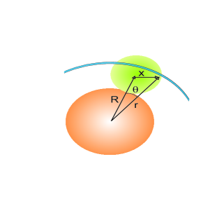
Figure 5: A spherical shell with radius $r$ from the center of the nucleus will have a contribution from the charge inside a nucleon located at a distance $R$.

The low energy expansion of the form factor, eq. 3, allows the extraction of the rms radius of the charge distribution from

$$\left\langle r_{ch}^{2}\right\rangle=-6\left[\frac{dF_{ch}}{d\left(q^{2}\right)}\right]_{q^{2}=0}.$$ (19)

Applying this relationship to the charge form factor used in figure 6 we get $\left\langle r_{ch}^{2}\right\rangle^{1/2}=2.82$ fm which is close to the experimental value $\left\langle r_{ch}^{2}\right\rangle_{\exp}^{1/2}=2.82\pm 0.06$ fm Blan97 . The shape of the charge form factor can also be described by a Gaussian distribution with radius parameter $a=2.30$ fm. In contrast to the case of ¹¹Li seen in figure 3, the proton halo in ⁸B does not seem to build up a two-Gaussian shaped form factor. This observation also seems to be in contradiction with the momentum distributions of ⁷Be fragments in knockout reactions using ⁸B projectiles in high energy collisions Schw95 . Electron scattering experiments will help to further elucidate this property of proton halos.

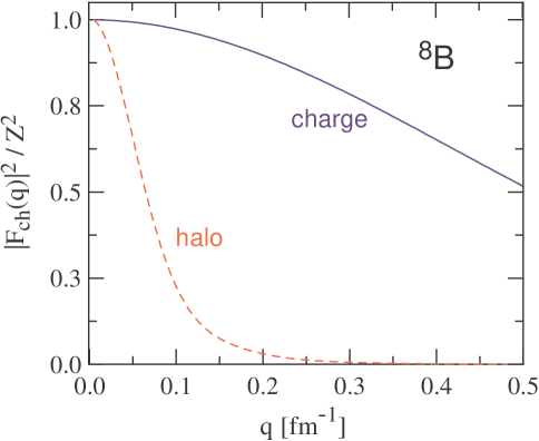
Figure 6: The charge form factor squared of ⁸B (solid line), $|F_{ch}^{total}(q)|^{2}/5^{2}$. Also shown is the charge form factor squared due only to the valence halo proton, $|F_{ch}^{halo}(q)|^{2}/1^{2}$.

III.4 Comparison with inelastic scattering

Loosely bound nuclei easily undergo breakup under any excitation. Such inelastic processes will always accompany elastic scattering. We follow the equations obtained in ref. Ber06 to make a crude estimate of the effects of inelastic electron scattering off loosely bound nuclei.

The inelastic cross section for the electro-excitation of loosely bound nuclei is given by Ber06

$$\frac{d\sigma_{\rm inel}}{d\Omega dE_{x}}=\frac{48\sqrt{2}}{\pi}\frac{e^{2}\left[e_{\mathrm{eff}}^{(1)}\right]^{2}p^{2}}{\hbar^{2}\mu c^{2}}\frac{1}{q^{2}}\frac{\sqrt{S_{n}}\left(E_{x}-S_{n}\right)^{3/2}}{E_{x}^{4}},$$ (20)

where $E_{x}$ is the excitation energy, $\Omega$ denotes the scattering solid angle, $e$ is the electron charge, $e^{(1)}_{\rm eff}$ is the electric effective charge for the nuclear response (I will assume for simplicity that $e^{(1)}_{\rm eff}$=$Ze$), and $S_{n}$ is the nuclear breakup energy. $p$ is the electron momentum, $q$ is the momentum transfer, and $\mu$ is the reduced mass, where it is assumed that the nucleus is composed of two clusters.

We now integrate this equation over the excitation energy $E_{x}$, and obtain

$$\frac{d\sigma_{\rm inel}}{d\Omega}=\frac{3\sqrt{2}}{4}\frac{Z^{2}e^{4}}{S_{n}\mu c^{2}}\frac{1}{\sin^{2}(\theta/2)}.$$ (21)

This equation is valid for large electron energies, so that $E\gg m_{e}c^{2}$, and for small scattering angles, for which the approximation $\hbar q\approx 2p\sin(\theta/2)$ can be used. In fact, the minimum momentum transfer for an excitation energy $E_{x}$ is given by $q_{\min}=\Delta k\cong E_{x}/\hbar c$. Thus, the inelastic cross section tends to a maximum value at very small scattering angles (in contrast, the elastic scattering cross section increases indefinitely at small angles). Equation 21 gives the behavior of the inelastic cross section when it starts to decrease with angle, shortly after the maximum at zero degrees. A characteristic feature emerging from eq. 21 is that the inelastic cross section is proportional to the inverse of the separation energy $S_{n}$.

From equation 1, neglecting nuclear recoil, one gets for the elastic scattering cross section $d\sigma_{\rm el}/d\Omega=Z^{2}e^{4}/4E^{2}\sin^{4}(\theta/2)$. The ratio between elastic and inelastic cross sections for small scattering angles is thus given by

$$\frac{d\sigma_{\rm el}}{d\sigma_{\rm inel}}=\frac{1}{3\sqrt{2}}\frac{S_{n}\mu c^{2}}{E^{2}}\frac{1}{\sin^{2}(\theta/2)}.$$ (22)

This shows that the elastic scattering dominates over inelastic scattering for $\theta\ll\theta_{\max}\approx\sqrt{S_{n}\mu c^{2}}/E$. Adopting typical values, i.e. $E=100$ MeV, $S_{n}=1$ MeV and $\mu c^{2}=10^{3}$ MeV, one gets $\theta_{\max}\approx 1/3$ radians. For $E=1$ GeV this value reduces to $\theta_{\max}\approx 1/30$ radians. These are kinematical constraints which have to be taken into account in future electron scattering experiments.

IV Inverse scattering problem

In PWBA the inverse scattering problem can be easily solved. It is possible to extract the form factor from the cross section and then, with an inversion of the Fourier transform, to get the charge density distribution

$$\rho_{ch}\left(r\right)=\frac{1}{2\pi^{2}}\int_{0}^{\infty}dq\ q^{2}j_{0}\left(qr\right)F_{ch}\left(q\right).$$ (23)

As we discussed in previous sections, the PWBA approximation can be justified only for light nuclei (e.g. ¹²C) in the region far from the diffraction zeros. For higher $Z$ values the agreement with experiment is only of a qualitative nature.

It is very common in the literature to use a theoretical model for $\rho_{ch}\left(r\right)$, e.g. the HF calculations discussed in the previous sections and compare the calculated $F(q)$ with experimental data. When the fit is “reasonable” (usually guided by the eye) the model is considered a good one. However, whereas the theoretical $\rho_{ch}\left(r\right)$ can contain useful information about the central part of the density (e.g. bubble-like nuclei, with a depressed central density), an excellent fit to the available experimental data does not necessarily mean that the data is sensitive to those details. The obvious reason is that short distances are probed by larger values of $q$. Experimental data from electron-ion colliders will suffer from limited accuracy at large values of $q$, possibly beyond $q=1$ fm^-1.  Thus it is useful to identify what are the conditions for reproducing the nuclear density within a theory independent fit.

In order to obtain an unbiased “experimental” $\rho_{ch}\left(r\right)$ one usually assumes that the density is expanded as

$$\rho_{ch}\left(r\right)=\sum_{n=1}^{\infty}a_{n}f_{n}\left(r\right),$$ (24)

where the basis functions $f_{n}(r)$ are drawn from any convenient complete set and the expansion coefficients $a_{n}$ are adjusted to reproduce the differential elastic cross section. The corresponding Fourier transform then takes the form

$$\widetilde{\rho}(q)\equiv F_{ch}\left(q\right)=\sum_{n=1}^{\infty}a_{n}\widetilde{f_{n}}\left(q\right),$$ (25)

where

$$\widetilde{f_{n}}\left(q\right)=4\pi\int_{0}^{\infty}dr\ r^{2}j_{0}\left(qr\right)f_{n}\left(r\right).$$ (26)

represents basis functions in momentum space.

Evidently the sum in eq. 24 has to be truncated and this produces an error in the determination of the charge density distribution. Another problem is that, as shown by eq. 23, the solution of the inverse scattering problem requires an accurate determination of the cross section up to large momentum transfers. Electron scattering experiments in electron-ion colliders will be performed within a limited range of $q$ and this will produce an uncertainty in the determination of the charge density distribution. As we have discussed in previous sections, the measurements have to encompass the first few minima of the cross section for heavy nuclei in order that the density profile can be mapped.

We consider two bases that have been found useful FN73 in the analysis of electron or proton scattering data. The present discussion is limited to spherical nuclei, but generalizations to deformed nuclei can be done. The Fourier-Bessel (FB) expansion (i.e. with $f_{n}$ taken as spherical Bessel functions) is useful because of the orthogonality relation between spherical Bessel functions

$$\int_{0}^{R_{\max}}dr\ r^{2}j_{l}\left(q_{n}r\right)j_{l}\left(q_{m}r\right)=\frac{1}{2}R_{c}^{3}\left[j_{l+1}\left(q_{n}R_{\max}\right)\right]^{2}\delta_{nm},$$ (27)

where the $q_{n}$ are defined such as

$$j_{l}\left(q_{n}R_{\max}\right)=0.$$ (28)

The FB basis implies that the charge density $\rho_{ch}(r)$ should be zero for values of $r$ larger than $R_{\max}$. For example, the basis can be defined as follows

$$f_{n}\left(r\right)=j_{0}\left(q_{n}r\right)\Theta\left(R_{\max}-r\right)\text{, \ \ \ \ \ \ \ \ \ \ \ \ \ }\widetilde{f_{n}}\left(q\right)=\frac{4\pi\left(-1\right)^{n}R_{\max}}{q^{2}-q_{n}^{2}}j_{0}\left(qR_{\max}\right)\text{, \ }$$ (29)

where $\Theta$ is the step function,  $R_{\max}$ is the expansion radius and $q_{n}=n\pi/R_{\max}$.

In principle it is possible to obtain the $a_{n}$ coefficients measuring directly the cross section at the $q_{n}$ momentum transfer. If the form factor (2) is known at $q_{n}$, the coefficients $a_{n}$ can be obtained inserting (27) and (29) in the definition (2) of the form factor, leading to

$$a_{n}=\frac{F_{ch}\left(q_{n}\right)}{2\pi R_{\max}^{3}\left[j_{1}\left(q_{n}R_{\max}\right)\right]^{2}}.$$ (30)

In general the cross sections  are measured at $q$ values different from $q_{n}$. Using the expansion (29) of the charge density one finds for the form factor the relation

$$F_{ch}\left(q\right)=\frac{4\pi}{q}\sum_{n}a_{n}\frac{\left(-1\right)^{n}}{q^{2}-q_{n}^{2}}\sin\left(qR_{\max}\right).$$ (31)

By fitting the experimental $F_{ch}(q)$ one obtains the $a_{n}$ parameters and reconstruct the nuclear charge density. Not all $a_{n}$’s are needed. Since the integral of the density, or $F\left(q=0\right)$, is fixed to the charge number there is one less degree of freedom. Also, densities tend to zero at large $r$. Thus another condition can be used, e.g. that the derivative of the density is zero at $R_{\max}$.  Thus, when we talk about $n$ expansion coefficients one means in fact that only $n-2$ coefficients need to be used in eq. 31. For experiments performed up to $q_{\max}$ the number of expansion coefficients needed for the fit is determined by $n_{\max}\simeq q_{\max}R_{\max}/\pi$.

A disadvantage of the FB expansion is that a relatively large number of terms is often needed to accurately represent a typical confined density, e.g. for light nuclei. One can use other expansion functions which are invoke less number of expansion parameters, e.g. the Laguerre-Gauss (LG) expansion,

$$f_{n}(r)=e^{-\alpha^{2}}L_{n}^{1/2}\left(2\alpha^{2}\right),\ \ \ \ \ \ \ \ \ \ \ \ \ \ \ \ \ \text{and}\ \ \ \ \widetilde{f_{n}}(q)=4\pi^{3/2}\beta^{3}\left(-1\right)^{n}e^{-\gamma^{2}}L_{n}^{1/2}\left(2\gamma^{2}\right),$$

where $\alpha=r/\beta$, $\gamma=q\beta/2$, and $L_{n}^{p}$ is the generalized Laguerre polynomial. Another possibility is to use an expansion on Hermite (H) polynomials. In both cases, the number of terms needed to provide a reasonable approximation to the density can be minimized by choosing $\beta$ in accordance with the natural radial scale. For light nuclei $\beta=1-2$ fm can be chosen, consistent with the parametrization of their densities. Then the magnitude of $a_{n}$ decreases rapidly with $n$, but the quality of the fit and the shape of the density are actually independent of $\beta$ over a wide range. As shown by application to a few cases, the main information on skin and halo sizes can be obtained using the FB expansion without problems.

Figure 7 shows the charge form factor squared for a Fermi function distribution with half-density radius $R=5.2$ fm and diffuseness $a=1.2$ fm (solid line). The dotted line is obtained with the FB expansion, eq. 31, up to $n=6$. The dashed curve uses up to $n=8$. One clearly sees that the latter improves the fit to the form factor up to the third minimum by increasing $n=6$ to $n=8$. We use $R_{\max}=15$ fm, so that adding the $n=8$ term improves the fit of the distribution including the peak at $q\simeq 1.75$ fm^-1, as seen in the figure.

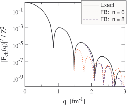
Figure 7: Form factor squared for a Fermi function charge distribution with half-density radius $R=5.2$ fm and diffuseness $a=1.2$ fm (solid line). The dotted line is obtained with the FB expansion, eq. 31, up to $n=6$. The dashed curve uses up to $n=8$.

For real data, the expansion coefficients $a_{n}$ are obtained by minimizing

$$\chi^{2}=\sum_{i}\left(\frac{y_{i}-y(q_{i},a_{n})}{\sigma_{i}}\right)^{2},$$

where $y(q_{i},a_{n})$ is the fitted value of the cross section (form factor) with a set of coefficients $a_{n}$ and $y_{i}$ are the experimental data at momentum $q_{i}$ with uncertainty $\sigma_{i}$.

To check the limitations of this procedure, we generate a set of pseudodata for ⁸B. The calculated charge form factor of figures 4 and 6 is used to generate 40 data points equally spaced by $\Delta q=0.02$ fm^-1.  These data were given an uncertainty $\sigma_{i}$ linearly increasing with $q_{i},$ from 1% for $q_{i}=0.02$ fm^-1 to 20% for $q_{i}=0.82$ fm^-1.

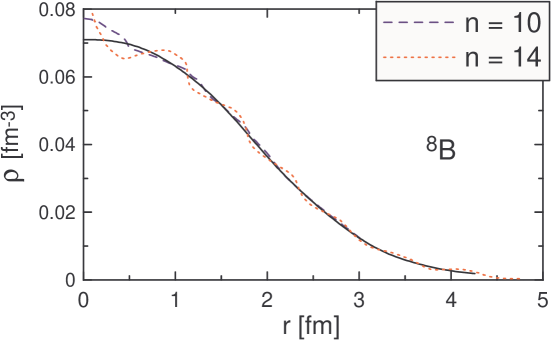
Figure 8: Hartree-Fock charge density of ⁸B (solid line). The dashed and dotted lines are the solution of the inverse scattering problem using a Fourier-Bessel expansion with $n=10$ and $n=14$ terms, respectively.

The best fit, with $R_{\max}=10$ fm, is obtained with $n=10$ expansion coefficients. Increasing the number of coefficients does not improve the quality of the fit, as is shown in figure 8 for $n=14$. It only produces more oscillations of the density. The reason is that terms with larger $n$’s are only needed to reproduce the data at larger values of momentum transfer, as shown in fig. 7. The fit to the data for $q<q_{\max}$ is not affected but the presence of these new terms introduces oscillations in the charge distribution. A possible fix to this problem is to include pseudodata in addition to experimental data. This method is well known in the literature FN73 . The pseudodata are used to enforce constraints and to estimate the incompleteness error associated with the limitation of experimental data to a finite range of momentum transfer.

V Conclusions

In this work I have studied the electron scattering off light unstable nuclei. This work is complementary to previous works in this area (see e.g. ref. GMG99 ; Ant05 ; Ers05 ; KA06 ). Particular attention was given to the effect of the neutron (proton) skin on the scattering form factors. It was shown that the position of the first minimum is arguably the best signature to look for noticeable changes in the charge radius size.

The evidence of a proton halo is not so clear as in the case of other probes. For example, it is well known that ⁷Be fragments arising from the proton knockout of ⁸B projectiles display a distinctively narrow momentum distribution characteristic of a long tail of the valence proton in ⁸B Schw95 . This feature is a consequence of the peripheral character of the knockout process, which is ideal to probe the tail of the bound states. Nonetheless, due to the Coulomb barrier the bulk of the charge in the nucleus is confined close to its center. Electron scattering is sensitive to this bulk charge and therefore does not display such a strong halo signature.

The minimum information obtained with electron scattering in electron-ion colliders will be the rms charge radius, $\left\langle r_{ch}^{2}\right\rangle^{1/2}$. This information “per se” is very valuable. It is sensitive to the skin size in a heavy nucleus. But it also depends on the accuracy with which this quantity can be measured. As we have shown in the previous sections, it will be necessary to go beyond the first minimum to extract information about the central value of the charge density.

Accurate measurements at large momentum transfers are crucial if one wants to describe the matter distribution with confidence and have a good comparison with predictions of different theoretical models. I have shown with a few basic examples using the Fourier-Bessel expansion method that, whereas the matter distribution within the halo is well probed by measurements at small momentum transfers, the details of the central distribution requires measurements at large $q$’s where inelastic processes may play an important role. This again imposes constraints on the information that can be extracted from elastic electron scattering off halo nuclei.

VI Appendix 1 - Analytical form factors

Here I summarize the analytical expressions for the charge form factors which are used in this work. For the nuclear charge density given by a hard sphere (uniform distribution with sharp cutoff at $R$)

$$\rho\left(r\right)=\left\{\begin{array}[c]{c}\rho_{0}\text{ \ \ \ \ \ for \ \ \ }r\leq R\\ 0\text{, \ \ \ \ \ \ \ otherwise,}\end{array}\right.$$ (32)

the form factor is

$$F(q)=\frac{4\pi\rho_{0}}{q^{3}}\left[\sin\left(qR\right)-qR\cos\left(qR\right)\right].$$ (33)

For an Yukawa distribution, $\rho\left(r\right)=\rho_{0}\ e^{-r/a}(a/r)$, one gets

$$F(q)=\frac{4\pi\rho_{0}a^{3}}{1+a^{2}q^{2}}.$$

The symmetrized Fermi distribution GLM91

$$\rho(r)=\rho_{0}\frac{\cosh(R/a)}{\cosh(R/a)+\cosh(r/a)}$$

leads to the form factor Co91 :

$$F(q)=-\frac{4\pi^{2}\rho_{0}a}{q}\frac{\cosh(R/a)}{\sinh(R/a)}\left[\frac{R\cos(qR)}{\sinh\left(\pi qa\right)}-\frac{\pi d\sin(qR)\cosh(\pi qa)}{\sinh^{2}\left(\pi qa\right)}\right].$$

The above expression is composed of oscillating terms damped by exponentials. This is better seen taking the limit for $qa\gg 1$:

$$F(q)\simeq-\frac{4\pi^{2}\rho_{0}a}{q}\left[R\cos(qR)-\pi a\sin(qR)\right]\ e^{-\pi qa}.$$ (34)

The Fermi distribution

$$\rho(r)=\rho_{0}/\left[1+\exp\left\{\left(r-R\right)/a\right\}\right]$$ (35)

with central density $\rho_{0}$, radius $R,$ and diffusiveness $a,$ gives a good description of the densities of heavy nuclei. This distribution can be fitted by the convolution $\rho\left(\mathbf{r}\right)=\int d^{3}r^{\prime}\rho_{p}\left(\mathbf{r}\right)\rho_{A}\left(\mathbf{r-r}^{\prime}\right)$ of a hard sphere for $\rho_{A}\left(\mathbf{r-r}^{\prime}\right)$ and an Yukawa function DN76 for $\rho_{p}\left(\mathbf{r}\right)$. The advantage is that the form factor factorizes, $F(q)=F_{p}(q)F_{A}(q)$, and can be calculated analytically as

$$F(q)=\frac{4\pi\rho_{0}}{q^{3}}\left[\sin\left(qR\right)-qR\cos\left(qR\right)\right]\left[\frac{1}{1+q^{2}a_{Y}^{2}}\right].$$ (36)

The term inside the first parenthesis comes from the hard sphere (uniform distribution with sharp cutoff at $R$) and the second parenthesis is the damping term due to an Yukawa diffuseness surface with width $a_{Y}$. Figure 9 compares $F(q)$ of eq. 36 with that obtained with the numerical integration of a two-point Fermi density distribution, eq. 35. The parameters for Al ($R=3.07$ fm , $a=0.519$ fm), Cu ($R=4.163$ fm , $a=0.606$ fm), Sn ($R=5.412$ fm , $a=0.560$ fm), Au ($R=$ 6.43 fm , $a=0.$ 541 fm) , and Pb ($R=6.62$ fm , $a=0.546$ fm) (to simplify the figure, I did not plot the curves for Au and Cu). In all cases I used for the Yukawa function parameter in eq. (36) $a_{Y}=0.7$ fm. We see that the agreement is very good.

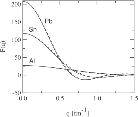
Figure 9: Comparison between form factors of a convoluted Fermi-Yukawa distribution calculated numerically using eq. 35 (solid lines), or with the analytical equation 36 (dashed lines).

For light nuclei, it is more appropriated to use Gaussian densities, with the Gaussian parameter $a=\sqrt{\frac{2}{3}\left\langle r^{2}\right\rangle_{ch}}$, where $\sqrt{\left\langle r^{2}\right\rangle_{ch}}$ is the root-mean-square radius of the matter density.  For example, for carbon, $a=2.018$ fm. For a Gaussian density parametrized as $\rho\left(r\right)=\rho_{0}\exp\left(-r^{2}/a^{2}\right)$, one gets

$$F(q)=\left(\pi a^{2}\right)^{3/2}\rho_{0}\exp\left(-q^{2}a^{2}/4\right)\;.$$ (37)

To simulate nodes in the wavefunctions of light nuclei, a sum of gaussian distributions can be used, including terms proportional to $r^{n}\exp\left(-r^{2}/a^{2}\right)$. The form factors arising from these terms can be obtained from nth-order derivatives of eq. 37 with respect to $1/a^{2}$.

For halo nuclei the following parametrization can be adopted

$$\rho\left(r\right)=\rho_{1}\exp\left(-r^{2}/a_{1}^{2}\right)+\rho_{2}\left(\frac{a_{2}}{r}\right)\exp\left(-r/a_{2}\right),$$ (38)

where the first term describes the density of the core and the second term describes the extended halo density. The second term blows up as $r\rightarrow 0$ and has only a meaning in the description of the long tail characterizing the halo wavefunction. If the core contains $A_{1}$ nucleons and the halo contains $A_{2}$ nucleons, the form factor for the above distribution becomes

$$F(q)=A_{1}\exp\left(-q^{2}a_{1}^{2}/4\right)+\frac{A_{2}}{1+a_{2}^{2}q^{2}}.$$ (39)

- (1) I. Tanihata et al., Phys. Rev. Lett. 55 (1985) 2676.
- (2) C.A. Bertulani, M.S. Hussein, and G. Münzenberg, Physics of Radioactive Beams (Nova Science Publishers, Hauppage, NY, 2002).
- (3) A. Ozawa, T. Suzuki and I. Tanihata, Nucl. Phys. A693 (2001) 32.
- (4) R. Hofstadter, Nobel Lectures, available at [http://nobelprize.org/physics/laureates/1961/hofstadter-lecture.pdf].
- (5) Technical Proposal for the Design, Construction, Commissioning, and Operation of the ELISe setup, spokesperson Haik Simon, GSI Internal Report, Dec. 2005.
- (6) T. Suda, K. Maruayama, Proposal for the RIKEN beam factory, RIKEN, 2001; M. Wakasugia, T. Suda, Y. Yano, Nucl. Inst. Meth. Phys. A 532, 216 (2004)
- (7) R. Hofstadter, Rev. Mod. Phys. 28, 214 (1956).
- (8) F. Hofmann and H. Lenske, Phys. Rev. C57, 2281 (1998).
- (9) S. Mizutori et al., Phys. Rev. C61, 0443261 (2000).
- (10) A.N. Antonov et al., Phys. Rev. C72, 044307 (2005).
- (11) E. Garrido and E. Moya de Guerra, Nucl. Phys. A650 (1999) 387; Phys. Lett. B488 (2000) 68.
- (12) S.N. Ershov, B.V. Danilin and J.S. Vaagen, Phys. Rev. C72, 044606 (2005).
- (13) S. Karataglidis and K. Amos, [arXiv:nucl-th/0609002].
- (14) R.F. Frosch et al., Phys. Rev. 174, 1380 (1968).
- (15) S. Galster et al., Nucl. Phys. B32(1971) 221 .
- (16) W.A. McKinley and H. Feshbach, Phys. Rev. 74, 1759 (1948).
- (17) D.R. Yennie, D.G. Ravenhall, and R.R. Wilson, Phys. Rev. 92, 1325 (1953); Phys. Rev. 95, 500 (1954).
- (18) L.S. Cutler, Phys. Rev. 157, 885 (1967).
- (19) J.M. Eisenberg and W. Greiner, “Excitation Mechanisms of the Nucleus”, (North-Holland, Amsterdam, 1988).
- (20) J. Dobaczewski,W. Nazarewicz, and T. R. Werner, Z. Phys. A 354, 27 (1996).
- (21) P. Danielewicz, Nucl. Phys. A 727 (2003) 233.
- (22) A.W. Steiner, M. Prakash, J.M. Lattimer, and P.J. Ellis, Phys. Rep. 411 (2005) 325.
- (23) A. Trzcinska et al., Phys. Rev. Lett. 87, 082501 (2001).
- (24) W. Schwab et al., Z. Phys. A350, 283 (1995).
- (25) G.F. Bertsch, A.B. Brown and H. Sagawa, Phys. Rev. C39, 1154 (1989).
- (26) H. Sagawa and C.A. Bertulani, Prog. Theo. Phys. Suppl. 124, 143 (1996).
- (27) H. Sagawa, Phys. Lett. B286 (1990) 7.
- (28) TUNL Nuclear Data Evaluation, [http://www.tunl.duke.edu/nucldata/].
- (29) P. Egelhof, Europ. Phys. Jour. A15 (2002) 27.
- (30) P. Bonche, S. Koonin and J. W. Negele, Phys. Rev. C13 (1976) 1226.
- (31) L.R. Sueltzle, M.R. Yearian, and H. Crannel, Phys. Rev. 162, 992 (1967).
- (32) S.S. Chandel, S.K. Dhiman and R. Shyam, Phys. Rev. C68, 054320 (2003).
- (33) E. Chabanat, P. Bonche, P. Haensel, J. Meyey and R. Schaeffer, Nucl. Phys. A627 (1997) 710.
- (34) P. Navratil, C.A. Bertulani and E. Caurier, Phys. Lett. B634 (2006) 191.
- (35) B. Blank et al., Nucl. Phys. A624 (1997) 242.
- (36) C.A. Bertulani, Phys. Lett. B624 (2005) 203.
- (37) J.L. Friar and J. W. Negele, Nucl. Phys. A212 (1973) 93.
- (38) K.T.R. Davies and J.R. Nix, Phys. Rev. C14, 1977 (1976).
- (39) M.E. Grypeos, G.A. Lalazissis, S.E. Massen and C.E Panos, J. Phys. G 17 (1991) 1093.
- (40) R.E. Kozak, Am. J. Phys. 59, 74 (1991).