Arbitrary $\ell$-state solutions of the rotating Morse potential by the asymptotic iteration method

Abstract

For non-zero $\ell$ values, we present an analytical solution of the radial Schrödinger equation for the rotating Morse potential using the Pekeris approximation within the framework of the Asymptotic Iteration Method. The bound state energy eigenvalues and corresponding wave functions are obtained for a number of diatomic molecules and the results are compared with the findings of the super-symmetry, the hypervirial perturbation, the Nikiforov-Uvarov, the variational, the shifted 1/N and the modified shifted 1/N expansion methods.

I Introduction

The Morse potential has raised a great deal of interest over the years and has been one of the most useful models to describe the interaction between two atoms in a diatomic molecule. It is known that the radial Schrödinger equation for this potential can be solved exactly when the orbital angular quantum number $\ell$ is equal to zero morse . On the other hand, it is also known that for $\ell\neq 0$, one has to use some approximations to find analytical or semi-analytical solutions. Several schemes have been presented for obtaining approximate solutions morales . Among these approximations, the most widely used and convenient one is the Pekeris approximation Pekeris ; fluge , which is based on the expansion of the centrifugal barrier in a series of exponentials depending on the internuclear distance up to the second order. Other approximations have also been developed to find better analytical formulas for the rotating Morse potential. However, all these approximations other than the Pekeris one require the calculation of a state-dependent internuclear distance through the numerical solutions of transcendental equations depristo ; elsum ; morales2 ; bag . In this respect, the rotating Morse potential has so far been solved by the super-symmetry (SUSY) susy ; morales , the Nikiforov-Uvarov method (NU) Nifikorov ; cuneyt , the shifted and modified shifted 1/N expansion methods bag ; expansion as well as the variational method variational using Pekeris approximations for $\ell\neq 0$. It is also solved by using the hypervirial perturbation method (HV) killingbeck with the full potential without Pekeris approximation.

In this paper, our aim is to solve the rotating Morse potential using a different and more practical method called, the asymptotic iteration method (AIM) hakanaim1 ; hakanaim2 within the Pekeris approximation and to obtain the energy eigenvalues and corresponding eigenfunctions. In the next section, the asymptotic iteration method (AIM) is introduced. Then, in section III, the Schrödinger equation is solved by the asymptotic iteration method with the non-zero angular momentum quantum numbers for the rotating Morse potential: The exact energy eigenvalues and corresponding wave functions are calculated for the $H_{2}$, $HCl$, $CO$ and $LiH$ diatomic molecules and AIM results are compared with the findings of the SUSY morales , the hypervirial perturbation method (HV) killingbeck , the Nikiforov-Uvarov method (NU) cuneyt and the shifted and modified shifted 1/N expansion methods bag ; expansion as well as with the variational method variational . Finally, section IV is devoted to the summary and conclusion.

II Basic Equations of the Asymptotic Iteration Method (AIM)

We briefly outline the asymptotic iteration method here and the details can be found in references hakanaim1 ; hakanaim2 . The asymptotic iteration method is proposed to solve the second-order differential equations of the form

$$y^{\prime\prime}=\lambda_{0}(x)y^{\prime}+s_{0}(x)y$$ (1)

where $\lambda_{0}(x)\neq 0$ and s₀(x), $\lambda_{0}$(x) are in C_∞(a,b). The variables, s₀(x) and $\lambda_{0}$(x), are sufficiently differentiable. The differential equation (1) has a general solution hakanaim1

$$y(x)=exp\left(-\int^{x}\alpha(x^{{}^{\prime}})dx^{{}^{\prime}}\right)\left[C_{2}+C_{1}\int^{x}exp\left(\int^{x^{{}^{\prime}}}(\lambda_{0}(x^{{}^{\prime\prime}})+2\alpha(x^{{}^{\prime\prime}}))dx^{{}^{\prime\prime}}\right)dx^{{}^{\prime}}\right]$$ (2)

if $k>0$, for sufficiently large $k$, we obtain the $\alpha(x)$ values from

$$\frac{s_{k}(x)}{\lambda_{k}(x)}=\frac{s_{k-1}(x)}{\lambda_{k-1}(x)}=\alpha(x),\quad k=1,2,3,\ldots$$ (3)

where

$$\lambda_{k}(x) = \lambda_{k-1}^{\prime}(x)+s_{k-1}(x)+\lambda_{0}(x)\lambda_{k-1}(x)\quad$$

$$s_{k}(x) = s_{k-1}^{\prime}(x)+s_{0}(x)\lambda_{k-1}(x),\quad\quad\quad\quad k=1,2,3,\ldots$$ (4)

The energy eigenvalues are obtained from the quantization condition. The quantization condition of the method together with equation (II) can also be written as follows

$$\delta_{k}(x)=\lambda_{k}(x)s_{k-1}(x)-\lambda_{k-1}(x)s_{k}(x)=0,\quad\quad k=1,2,3,\ldots$$ (5)

For a given potential such as the rotating Morse one, the radial Schrödinger equation is converted to the form of equation (1). Then, s${}_{0}(x)$ and $\lambda_{0}(x)$ are determined and s${}_{k}(x)$ and $\lambda_{k}(x)$ parameters are calculated. The energy eigenvalues are determined by the quantization condition given by equation (5). However, the wave functions are determined by using the following wave function generator

$$y_{n}(x)=C_{2}exp(-\int^{x}\frac{s_{k}(x^{\prime})}{\lambda_{k}(x^{\prime})}dx^{\prime})$$ (6)

III Calculation of the Energy Eigenvalues and Eigenfunctions

The motion of a particle with the reduced mass $\mu$ is described by the following Schrödinger equation:

$$\frac{-\hbar^{2}}{2\mu}\left(\frac{\partial^{2}}{\partial r^{2}}+\frac{2}{r}\frac{\partial}{\partial r}+\frac{1}{r^{2}}\left[\frac{1}{\sin\theta}\frac{\partial}{\partial\theta}\left(\sin\theta\frac{\partial}{\partial\theta}\right)+\frac{1}{\sin^{2}\theta}\frac{\partial^{2}}{\partial\phi^{2}}\right]+V(r)\right)\Psi_{n\ell m}(r,\theta,\phi)=E\Psi_{n\ell m}(r,\theta,\phi)$$ (7)

The terms in the square brackets with the overall minus sign are the dimensionless angular momentum squared operator, ${\bf L}^{2}$. Defining $\Psi_{n\ell m}(r,\theta,\phi)=u_{n\ell}(r)Y_{\ell m}(\theta,\phi)$, we obtain the radial part of the Schrödinger equation:

$$\left(\frac{d^{2}}{d{r}^{2}}+\frac{2}{r}\frac{d}{dr}\right)u_{n\ell}(r)-\frac{2\mu}{\hbar^{2}}\left[V(r)+\frac{\ell(\ell+1)\hbar^{2}}{2\mu r^{2}}\right]u_{n\ell}(r)+\frac{2\mu E}{\hbar^{2}}u_{n\ell}(r)=0$$ (8)

It is sometimes convenient to define $u_{n\ell}(r)$ and the effective potential as follows:

$$u_{n\ell}(r)=\frac{R_{n\ell}(r)}{r},\quad V_{eff}=V(r)+\frac{\ell(\ell+1)\hbar^{2}}{2\mu r^{2}}$$ (9)

Since

$$\left(\frac{d^{2}}{d{r}^{2}}+\frac{2}{r}\frac{d}{dr}\right)\frac{R_{n\ell}(r)}{r}=\frac{1}{r}\frac{d^{2}}{d{r}^{2}}R_{n\ell}(r)$$ (10)

The radial Schrödinger equation given by equation (8) follows that

$$\frac{d^{2}R_{n\ell}(r)}{d{r}^{2}}+\frac{2\mu}{\hbar^{2}}\left[E-V_{eff}\right]R_{n\ell}(r)=0$$ (11)

Instead of solving the partial differential equation (7) in three variables $r$, $\theta$ and $\phi$, we now solve a differential equation involving only the variable $r$, but dependent on the angular momentum parameter $\ell$, which makes the solution of this equation difficult for $\ell\neq 0$ or sometimes impossible within a given potential.

The Morse potential we examine in this paper is defined as

$$V_{Morse}(r)=D\left(e^{-2\alpha x}-2e^{-\alpha x}\right)$$ (12)

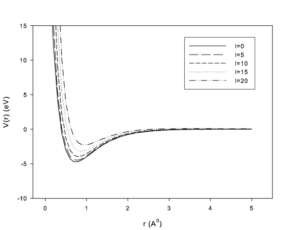
Figure 1: The shape of the rotating Morse potential for $H_{2}$ diatomic molecule is plotted against the separation $r$ for different orbital angular momentum quantum numbers.

with $x=(r-r_{e})/r_{e}$ and $\alpha=ar_{e}$. Here, $D$ and $\alpha$ denote the dissociation energy and Morse parameter, respectively. $r_{e}$ is the equilibrium distance (bound length) between nuclei and $a$ is a parameter to control the width of the potential well. For the $H_{2}$ diatomic molecule, the effective potential, which is the sum of the centrifugal and Morse potentials, is shown in figure 1 for various values of the orbital angular momentum. The superposition of the attractive and repulsive potentials results in the formation of a potential pocket, whose the width and depth depend on the orbital angular momentum quantum number for a given molecular potential. The potential pocket becomes shallower as the orbital angular momentum quantum number $\ell$ increases, which also indicates that the number of states supported by the potential decreases. This pocket is also very important for the scattering case due to the interference of the barrier and internal waves, which creates the oscillatory structure in the cross-section. The effect of this pocket can be understood in terms of the interference between the internal and barrier waves that corresponds to a decomposition of the scattering amplitude into two components, the inner and external waves Lee78 ; Bri77 ; Bozosi .

The effective potential together with the Morse potential for $\ell\neq 0$ can be written as,

$$V_{eff}(r)=V_{\ell}(r)+V_{Morse}(r)=\frac{\ell(\ell+1)\hbar^{2}}{2\mu r^{2}}+D\left(e^{-2\alpha x}-2e^{-\alpha x}\right)$$ (13)

It is known that the Schrödinger equation cannot be solved exactly for this potential for $\ell\neq 0$ by using the standard methods such as SUSY and NU. As it is seen from equation (13), the effective potential is a combination of the exponential and inverse square potentials, which cannot be solved analytically. Therefore, an approximation has to be made: The most widely used and convenient one is the Pekeris approximation. This approximation is based on the expansion of the centrifugal barrier in a series of exponentials depending on the internuclear distance, keeping terms up to second order, so that the effective $\ell$-dependent potential keeps the same form as the potential with $\ell$=0 morales . It should be pointed out, however, that this approximation is valid only for low vibrational energy states. In the Pekeris approximation, by change of the coordinates $x=(r-r_{e})/r_{e}$, the centrifugal potential is expanded in a series around $x=0$

$$V_{\ell}(x)=\frac{\ell(\ell+1)\hbar^{2}}{2\mu r_{e}^{2}}\frac{1}{(1+x)^{2}}=\gamma(1-2x+3x^{2}-4x^{3}+...)$$ (14)

where $\gamma=\frac{\ell(\ell+1)\hbar^{2}}{2\mu r_{e}^{2}}$. Taking up to the second order degrees in this series and writing them in terms of exponentials, we get

$$\widetilde{V}_{\ell}(x)=\gamma\left(c_{0}+c_{1}e^{-\alpha x}+c_{2}e^{-2\alpha x}\right)$$ (15)

In order to determine the constants $c_{0}$, $c_{1}$ and $c_{2}$, we also expand this potential in a series of $x$

$$\widetilde{V}_{\ell}(x)=\gamma\left(c_{0}+c_{1}+c_{2}-(c_{1}+2c_{2})\alpha x+(\frac{c_{1}}{2}+2c_{2})\alpha^{2}x^{2})\ldots\right)$$ (16)

Comparing equal powers of equations (14) and (16), we obtain the constants $c_{0}$, $c_{1}$ and $c_{2}$ as,

$$c_{0}=1-\frac{3}{\alpha}+\frac{3}{\alpha^{2}},\quad c_{1}=\frac{4}{\alpha}-\frac{6}{\alpha^{2}},\quad c_{2}=-\frac{1}{\alpha}+\frac{3}{\alpha^{2}}$$ (17)

Now, the effective potential with Pekeris approximation becomes,

$$\widetilde{V}_{eff}(x)=\gamma(c_{0}+c_{1}e^{-\alpha x}+c_{2}e^{-2\alpha x})+D\left(e^{-2\alpha x}-2e^{-\alpha x}\right)$$ (18)

Instead of solving the radial Schrödinger equation for the effective potential given by equation (13), we solve the radial Schrödinger equation for the new effective potential given by equation (18) obtained by using the Pekeris approximation. Inserting this effective potential equation (18) into equation (11) and using the following ansatzs

$$-\varepsilon^{2}=\frac{2\mu r_{e}^{2}}{\hbar^{2}}(E-\gamma c_{0}),\quad\beta_{1}^{2}=\frac{2\mu r_{e}^{2}}{\hbar^{2}}(2D-\gamma c_{1}),\quad\beta_{2}^{2}=\frac{2\mu r_{e}^{2}}{\hbar^{2}}(\gamma c_{2}+D)$$ (19)

The radial Schrödinger equation takes the following form:

$$\frac{d^{2}R_{n\ell}(x)}{dx^{2}}+\left(-\varepsilon^{2}+\beta_{1}^{2}e^{-\alpha x}-\beta_{2}^{2}e^{-2\alpha x}\right)R_{n\ell}(x)=0$$ (20)

If we rewrite equation (20) by using a new variable of the form $y=e^{-\alpha x}$, we obtain

$$\frac{d^{2}R_{n\ell}(y)}{dy^{2}}+\frac{1}{y}\frac{dR_{n\ell}(y)}{dy}+\left[-\frac{\varepsilon^{2}}{\alpha^{2}}\frac{1}{y^{2}}+\frac{\beta_{1}^{2}}{\alpha^{2}}\frac{1}{y}-\frac{\beta_{2}^{2}}{\alpha^{2}}\right]R_{n\ell}(y)=0$$ (21)

In order to solve this equation with AIM for $\ell\neq 0$, we should transform this equation to the form of equation (1). Therefore, the reasonable physical wave function we propose is as follows

$$R_{n\ell}(y)=y^{\frac{\varepsilon}{\alpha}}e^{-\frac{\beta_{2}}{\alpha}y}f_{n\ell}(y)$$ (22)

If we insert this wave function into the equation (21), we have the second-order homogeneous linear differential equations in the following form

$$\frac{d^{2}f_{n\ell}(y)}{dy^{2}}=\left(\frac{2\beta_{2}\alpha y-2\varepsilon\alpha-\alpha^{2}}{y\alpha^{2}}\right)\frac{df_{n\ell}(y)}{dy}+\left(\frac{2\varepsilon\beta_{2}+\alpha\beta_{2}-\beta_{1}^{2}}{y\alpha^{2}}\right)f_{n\ell}(y)$$ (23)

which is now amenable to an AIM solution. By comparing this equation with equation (1), we can write the $\lambda_{0}(y)$ and $s_{0}(y)$ values and by means of equation (II), we may calculate $\lambda_{k}(y)$ and $s_{k}(y)$. This gives (the subscripts are omitted):

$$\lambda_{0} = \left(\frac{2\beta_{2}y-2\varepsilon-\alpha}{\alpha y}\right)$$

$$s_{0} = \left(\frac{2\varepsilon\beta_{2}+\alpha\beta_{2}-\beta_{1}^{2}}{\alpha^{2}y}\right)$$

$$\lambda_{1} = {\frac{-3\,\beta_{2}\,\alpha\,y+6\,\alpha\,\varepsilon+2\,{\alpha}^{2}-6\,y\varepsilon\,\beta_{2}-y{\beta_{1}}^{2}+4\,{\beta_{2}}^{2}{y}^{2}+4\,{\varepsilon}^{2}}{{\alpha}^{2}{y}^{2}}}$$

$$s_{1} = 2\,{\frac{\left(2\,\varepsilon\,\beta_{2}+\alpha\,\beta_{2}-{\beta_{1}}^{2}\right)\left(-\alpha+\beta_{2}\,y-\varepsilon\right)}{{\alpha}^{3}{y}^{2}}}$$ (24)

$$\ldots\emph{etc}$$

Combining these results with the quantization condition given by equation (5) yields

$$\frac{s_{0}}{\lambda_{0}} = \frac{s_{1}}{\lambda_{1}}\,\,\,\,\,\,\Rightarrow\,\,\,\,\,\,\varepsilon_{0}=-\frac{1}{2}\frac{\alpha\beta_{2}-\beta_{1}^{2}}{\beta_{2}}$$

$$\frac{s_{1}}{\lambda_{1}} = \frac{s_{2}}{\lambda_{2}}\,\,\,\,\,\,\Rightarrow\,\,\,\,\,\,\varepsilon_{1}=-\frac{1}{2}\frac{3\alpha\beta_{2}-\beta_{1}^{2}}{\beta_{2}}$$

$$\frac{s_{2}}{\lambda_{2}} = \frac{s_{3}}{\lambda_{3}}\,\,\,\,\,\,\Rightarrow\,\,\,\,\,\,\varepsilon_{2}=-\frac{1}{2}\frac{5\alpha\beta_{2}-\beta_{1}^{2}}{\beta_{2}}$$ (25)

$$\ldots\emph{etc}$$

When the above expressions are generalized, the eigenvalues turn out as

$$\varepsilon_{n\ell}=\frac{\beta_{1}^{2}-(2n+1)\alpha\beta_{2}}{2\beta_{2}},\hskip 28.45274ptn=0,1,2,3,...$$ (26)

Using equation (19), we obtain the energy eigenvalues E_nℓ,

$$E_{n\ell}=-\frac{\hbar^{2}}{2\mu r_{e}^{2}}\left[\frac{\beta_{1}^{2}}{2\beta_{2}}-(n+\frac{1}{2})\alpha\right]^{2}+\gamma c_{0}$$ (27)

As it is seen that the energy eigenvalue equation is easily obtained by using AIM. This is the advantage of the AIM that it gives the eigenvalues directly by transforming the radial Schrödinger equation into a form of ${y}^{\prime\prime}$ =$\lambda_{0}(r){y}^{\prime}+s_{0}(r)y$. In order to test the accuracy of equation (27), we calculate the energy eigenvalues of the $H_{2}$, $HCl$, $CO$ and $LiH$ diatomic molecules. The AIM results are compared with those obtained by SUSY method morales using original Pekeris approximation, the hypervirial perturbation method (HV) killingbeck , the shifted 1/N and modified shifted 1/N expansion methods bag for the $H_{2}$ diatomic molecule in Table 1. In Table 2, we show the same comparison for the $HCl$ diatomic molecule. Furthermore, the AIM results are compared with those obtained by NU method cuneyt , shifted 1/N and modified shifted 1/N expansion methods bag for the $CO$ and $LiH$ diatomic molecules in Tables 3 and 4, respectively. As it can be seen from the results presented in these tables that the AIM results are in good agreement with the findings of the other methods.

After we find the energy eigenvalues, the following wave function generator can be used to find $f_{n}(y)$ functions by using AIM

$$f_{n}(y)=exp(-\int^{y}\frac{s_{k}}{\lambda_{k}}dy^{\prime})$$ (28)

where $n$ represents the radial quantum number and $k$ shows the iteration number. Below, the first few $f(y)$ functions can be seen

$$f_{0}(y) = 1$$ (29)

$$f_{1}(y) = (2\alpha\beta_{2}-\beta_{1}^{2})\left(1-\frac{2\beta_{2}y}{\alpha(\frac{\beta 1^{2}-3\alpha\beta_{2}}{\alpha\beta_{2}}+1)}\right)$$ (30)

$$f_{2}(y) = (\beta_{1}^{2}-4\alpha\beta_{2})(\beta_{1}^{2}-3\alpha\beta_{2})\left(1-\frac{4\beta_{2}y}{\alpha(\frac{\beta_{1}^{2}-5\alpha\beta_{2}}{\alpha\beta_{2}}+1)}+\frac{4\beta_{2}^{2}y^{2}}{\alpha^{2}(\frac{\beta_{1}^{2}-5\alpha\beta_{2}}{\alpha\beta_{2}}+1)(\frac{\beta_{1}^{2}-5\alpha\beta_{2}}{\alpha\beta_{2}}+2)}\right)$$ (31)

$$f_{3}(y) = (-4\alpha\beta_{2}+\beta_{1}^{2})(\beta_{1}^{2}-5\alpha\beta_{2})(\beta_{1}^{2}-6\alpha\beta_{2})\left(1-\frac{6\beta_{2}y}{\alpha(\frac{\beta_{1}^{2}-7\alpha\beta_{2}}{\beta_{2}\alpha}+1)}\right.$$ (32)

$$+ \left.\frac{12\beta_{2}^{2}y^{2}}{\alpha^{2}(\frac{\beta_{1}^{2}-7\alpha\beta_{2}}{\alpha\beta_{2}}+1)(\frac{\beta_{1}^{2}-7\alpha\beta_{2}}{\alpha\beta_{2}}+2)}-\frac{8\beta_{2}^{3}y^{3}}{\alpha^{3}(\frac{\beta_{1}^{2}-7\alpha\beta_{2}}{\alpha\beta_{2}}+1)(\frac{\beta_{1}^{2}-7\alpha\beta_{2}}{\alpha\beta_{2}}+2)(\frac{\beta_{1}^{2}-7\alpha\beta_{2}}{\alpha\beta_{2}}+3)}\right)$$

$$\ldots\emph{etc}$$

It can be understood from the results given above that we can write the general formula for $f_{n}(y)$ as follows,

$$f_{n}(y)=(-1)^{n}\left(\prod\limits_{k=n}^{2n-1}(\beta_{1}^{2}-(k+1)\alpha\beta_{2})\right){{}_{1}}F_{1}(-n,\frac{2\varepsilon_{n}}{\alpha}+1;\frac{2\beta_{2}y}{\alpha})$$ (33)

Thus, we can write the total radial wave function as below,

$$R_{n\ell}=(-1)^{n}\left(\prod\limits_{k=n}^{2n-1}(\beta_{1}^{2}-(k+1)\alpha\beta_{2})\right)y^{\frac{\varepsilon_{n}}{\alpha}}e^{-\frac{\beta_{2}}{\alpha}y}{{}_{1}}F_{1}(-n,\frac{2\varepsilon_{n}}{\alpha}+1;\frac{2\beta_{2}y}{\alpha})$$ (34)

When the hypergeometric function is written in terms of the Laguerre polynomials, we get

$$R_{n\ell}=Ny^{\frac{\varepsilon_{n}}{\alpha}}e^{-\frac{\beta_{2}}{\alpha}y}L_{n}^{\frac{2\varepsilon_{n}}{\alpha}}\left(\frac{2\beta_{2}}{\alpha}y\right)$$ (35)

Where $N$ is the normalization constant and can be obtained from $N^{2}\int\limits_{0}^{\infty}y^{\frac{2\varepsilon_{n}}{\alpha}}e^{-\frac{2\beta_{2}}{\alpha}y}\left[L_{n}^{\frac{2\varepsilon_{n}}{\alpha}}(\frac{2\beta_{2}}{\alpha}y)\right]^{2}dy=1$ as below,

$$N=\frac{1}{n!}\left(\frac{2\beta_{2}}{\alpha}\right)^{\frac{\xi+1}{2}}\sqrt{\frac{(n-\xi)!}{n!}}$$ (36)

where $\xi=\frac{2\varepsilon_{n}}{\alpha}$.

IV Conclusion

We have shown an alternative method to obtain the energy eigenvalues and corresponding eigenfunctions of the rotating Morse potential using Pekeris approximation within the framework of the asymptotic iteration method. The main results of this paper are the energy eigenvalues and eigenfunctions, which are given by equations (27) and (35) respectively. The energy eigenvalues are obtained for the $H_{2}$, $HCl$, $CO$ and $LiH$ diatomic molecules. Our AIM results are compared with the findings of the other methods such as the SUSY morales , the hypervirial perturbation method (HV) killingbeck , the Nikiforov-Uvarov method (NU) cuneyt and the shifted and modified shifted 1/N expansion methods bag ; expansion as well as the variational method variational in Tables 1, 2, 3 and 4. The advantage of the asymptotic iteration method is that it gives the eigenvalues directly by transforming the radial Schrödinger equation into a form of ${y}^{\prime\prime}$ =$\lambda_{0}(r){y}^{\prime}+s_{0}(r)y$. The wave functions are easily constructed by iterating the values of $s_{0}(r)$ and $\lambda_{0}(r)$. The method presented in this study is a systematic one and it is very efficient and practical. It is worth extending this method to the solution of other interaction problems.

		AIM	SUSY	HV	Variational	Modified Shifted 1/N	Shifted 1/N
$n$	$\ell$	results	results	results	results	expansion results	expansion results
0	0	-4.47601	-4.47601	-4.47601	-4.4758	-4.4760	-4.4749
	5	-4.25880	-4.25880	-4.25901	-4.2563	-4.2590	-4.2590
	10	-3.72193	-3.72193	-3.72473	-3.7187	-3.7247	-3.7247
5	0	-2.22052	-2.22051	-2.22051	-	-2.2205	-2.2038
	5	-2.04355	-2.04353	-2.05285	-	-2.0530	-2.0525
	10	-1.60391	-1.60389	-1.65265	-	-1.6535	-1.6526
7	0	-1.53744	-1.53743	-1.53743	-	-1.5374	-1.5168
	5	-1.37656	-1.37654	-1.39263	-	-1.3932	-1.3887
	10	-0.97581	-0.97578	-1.05265	-	-1.0552	-1.0499

Table 1: For the $H_{2}$ diatomic molecule, the comparison of the energy eigenvalues (in eV) obtained by using AIM with other methods for different values of $n$ and $\ell$. Potential parameters are $D~{}=~{}4.7446eV$, $a=1.9425(A^{0})^{-1}$, $r_{e}=0.7416A^{0}$, ${\hbar c}=1973.29eVA^{0}$ and $\mu=0.50391$amu.

		AIM	Variational	Modified Shifted 1/N	Shifted 1/N
$n$	$\ell$	results	results	expansion results	expansion results
0	0	-4.4356	-4.4360	-4.4355	-4.4352
	5	-4.3968	-4.3971	-4.3968	-4.3967
	10	-4.2941	-4.2940	-4.2940	-4.2939
5	0	-2.8051	-	-2.8046	-2.7727
	5	-2.7721	-	-2.7718	-2.7508
	10	-2.6847	-	-2.6850	-2.6712
7	0	-2.2570	-	-2.2565	-2.2002
	5	-2.2263	-	-2.2262	-2.1874
	10	-2.1451	-	-2.1461	-2.1194

Table 2: For the $HCl$ diatomic molecule, the comparison of the energy eigenvalues (in eV) obtained by using AIM with other methods for different values of $n$ and $\ell$. Potential parameters are $D=37255cm^{-1}$, $a=1.8677(A^{0})^{-1}$, $r_{e}=1.2746A^{0}$, ${\hbar c}=1973.29eVA^{0}$ and $\mu=0.9801045$amu.

				AIM		NU		Variational		Modified Shifted 1/N		Shifted 1/N
$n$		$\ell$		results		results		results		expansion results		expansion results
0		0		-11.0915		-11.091		-11.093		-11.092		-11.091
		5		-11.0844		-11.084		-11.085		-11.084		-11.084
		10		-11.0653		-11.065		-11.066		-11.065		-11.065
5		0		-9.7952		-9.795		-		-9.795		-9.788
		5		-9.7883		-9.788		-		-9.788		-9.782
		10		-9.7701		-9.769		-		-9.770		-9.765
7		0		-9.2992		-9.299		-		-9.299		-9.286
		5		-9.2925		-9.292		-		-9.292		-9.281
		10		-9.2745		-9.274		-		-9.274		-9.265

Table 3: For the $CO$ diatomic molecule, the comparison of the energy eigenvalues (in eV) obtained by using AIM with other methods for different values of $n$ and $\ell$. Potential parameters are $D=90540cm^{-1}$, $a=2.2994(A^{0})^{-1}$, $r_{e}=1.1283A^{0}$, ${\hbar c}=1973.29eVA^{0}$ and $\mu=6.8606719$amu.

				AIM		NU		Variational		Modified Shifted 1/N		Shifted 1/N
$n$		$\ell$		results		results		results		expansion results		expansion results
0		0		-2.4289		-2.4287		-2.4291		-2.4280		-2.4278
		5		-2.4013		-2.4012		-2.4014		-2.4000		-2.3999
		10		-2.3288		-2.3287		-2.3287		-2.3261		-2.3261
5		0		-1.6477		-1.6476		-		-1.6402		-1.6242
		5		-1.6238		-1.6236		-		-1.6160		-1.6074
		10		-1.5607		-1.5606		-		-1.5525		-1.5479
7		0		-1.3776		-1.3774		-		-1.3682		-1.3424
		5		-1.3550		-1.3549		-		-1.3456		-1.3309
		10		-1.2958		-1.2957		-		-1.2865		-1.2781

Table 4: For the $LiH$ diatomic molecule, the comparison of the energy eigenvalues (in eV) obtained by using AIM with other methods for different values of $n$ and $\ell$. Potential parameters are $D=20287cm^{-1}$, $a=1.1280(A^{0})^{-1}$, $r_{e}=1.5956A^{0}$, ${\hbar c}=1973.29eVA^{0}$ and $\mu=0.8801221$amu.

References

- (1) P. M. Morse, Phys. Rev. 34 (1929) 57.
- (2) D. A. Morales, Chem. Phys. Letters 394 (2004) 68.
- (3) C. L. Pekeris, Phys. Rev. 45 (1934) 98.
- (4) S. Flügge, Practical Quantum Mechanics Vol. I, Springer, Berlin, (1994).
- (5) A.E. DePristo, J. Chem. Phys. 74 (1981) 5037.
- (6) J.R. Elsum and G. Gordon, J. Chem. Phys. 76 (1982) 5452.
- (7) D.A. Morales, Chem. Phys. Lett. 161 (1989) 253.
- (8) M. Bag et al., Phys. Rev. A46, (1992) 9.
- (9) F. Cooper, A. Khare and U. Sukhatme, Phys. Rep. 251 (1995) 267.
- (10) A. F. Nikiforov and V. B. Uvarov, Special Functions of Mathematical Physics, Birkhäuser, Basel, (1988).
- (11) C. Berkdemir and J. Han, Chem. Phys. Letters, 409 (2005) 203.
- (12) T. Imbo and U. Sukhatme, Phys. Rev. Lett. 54 (1985) 2184.
- (13) E. D. Filho and R. M. Ricotta, Phys. Lett. A269 (2000) 269.
- (14) J.P. Killingbeck, A. Grosjean and G. Jolicard, J. Chem. Phys. 116 (2002) 447.
- (15) H. Ciftci, R. L. Hall and N. Saad, J. Phys. A: Math. Gen. 36 (2003) 11807.
- (16) H. Ciftci, R. L. Hall and N. Saad, Phys. Lett. A340 (2005) 388.
- (17) S.Y. Lee, Nucl. Phys. A311 (1978) 518.
- (18) D.M. Brink and N. Takigawa, Nucl. Phys. A279 (1977) 159.
- (19) I. Boztosun, Phys. Rev. C 66 (2002) 024610.