Relativistic effects in exclusive neutron-deuteron breakup

Abstract

We extended the study of relativistic effects in neutron-deuteron scattering to the exclusive breakup. To this aim we solved the three-nucleon Faddeev equation including such relativistic features as relativistic kinematics and boost effects at incoming neutron lab. energies $E_{n}^{lab}=65$ MeV, $156$ MeV and $200$ MeV. As dynamical input a relativistic nucleon-nucleon interaction exactly on-shell equivalent to the CD Bonn potential has been used. We found that the magnitude of relativistic effects increases with the incoming neutron energy and, depending on the phase-space region, relativity can increase as well as decrease the nonrelativistic breakup cross section. In some regions of the breakup phase-space dynamical boost effects are important. For a number of measured exclusive cross sections relativity seems to improve the description of data.

I Introduction

The high precision nucleon-nucleon (NN) potentials which describe very well the NN data set up to about $350$ MeV AV18 ; CDBONN ; NIJMI form a very firm basis for a study of three-nucleon (3N) reactions. Powerful computers and development of modern algorithms provided numerically exact solutions of the 3N Schrödinger equation both in the momentum and coordinate representation. This permitted theoretical calculations for cross sections and spin observables in elastic nucleon-deuteron (Nd) scattering and breakup processes with different dynamical assumptions about underlying nuclear forces glo96 . With increasing amount of precise 3N elastic scattering data it turned out, that nonrelativistic description based on pairwise forces only is insufficient to explain the data at higher energies of the 3N system. Adding a 3N force (3NF) to the pairwise interactions led in many cases to a better description of the data wit98 ; sek02 ; wit01 ; abf98 ; wit99 ; hat02 ; cad01 ; bieber2000 ; erm2001 ; erm2003 ; erm2005 . However, at energies higher than $\approx 100$ MeV current 3NFs only partially improved the description of data, leaving in some cases discrepancies which were comparable in magnitude to the effects of the 3NFs themselves sek02 ; wit01 ; abf98 ; wit99 ; hat02 ; cad01 ; bieber2000 ; erm2001 ; erm2003 ; erm2005 .

This situation triggered investigations of the 3N continuum taking relativistic effects into account. In ref. witrel we performed such a study for Nd elastic scattering. We extended the Hamiltonian scheme in equal time formulation worked out in kam2002 to the 3N scattering taking as a starting point the Lorentz boosted NN potential which generates the NN t-matrix in a moving frame via a standard Lippmann-Schwinger equation. The NN potential in an arbitrary moving frame is based on the interaction in the two-nucleon c.m. system, which enters a relativistic NN Schrödinger or Lippmann-Schwinger equation. The relativistic equation differs from the nonrelativistic one just by the relativistic form of the kinetic energy. We constructed the relativistic two nucleon (2N) potential by performing an analytical scale transformation of momenta, which relates NN potentials in the nonrelativistic and relativistic Schrödinger equations in such a way, that exactly the same NN phase shifts are obtained by both equations kam98 .

In our first study witrel we looked for changes in elastic neutron-deuteron (nd) scattering observables when the nonrelativistic form of the kinetic energy was replaced by the relativistic one and a proper treatment of boost effects and Wigner rotations of spin states was included. It turned out, that the effects of spin rotations in the studied energy range up to $250$ MeV were practically negligible for elastic scattering cross sections and analyzing powers. The relativistic effects for the elastic scattering cross section were significant only at higher energies and restricted to the very backward angles, where relativity increased the nonrelativistic cross section. The decisive role was played by the boost effects which reduced the transition matrix elements at higher energies and led, in spite of the increased elastic scattering relativistic phase-space factor as compared to the nonrelativistic one, to rather small effects in the cross section.

In view of upcoming measurements of the higher energy Nd breakup process we would like to extend the study of ref. witrel to this reaction. The first results presented in wit2006 revealed a unique selectivity of the complete breakup reaction useful to investigate the pattern of relativistic effects and to study their significance. Here we would like to study how relativistic effects are distributed over the breakup phase-space and if and to what extent the existing data verify the predicted effects.

The paper is organized as follows. In Sec. II for convenience of the reader we shortly explain the relativistic features underlying our treatment of a relativized Faddeev equation in the 3N continuum. The very detailed presentation which incorporated the definition of the boosted two-body force, the various two-and three-body states in general frames, the Wigner rotations and the singularity structure of the relativistic free 3N propagator were given in witrel . In Sec. III we give relativistic and nonrelativistic formulas for the transition matrix elements and the breakup cross section. In Sec. IV we apply our formulation using a relativistic NN interaction which is exactly on-shell equivalent to the nonrelativistic CD Bonn potential and solve the relativized 3N Faddeev equation with different approximations for the boost. At two incoming neutron energies, 65 and 200 MeV, we look for the magnitude and the distribution pattern of relativistic effects over the entire phase-space of the breakup reaction. For the cases where the data are available, we compare them to theoretical predictions. Finally, Sec. V contains a summary and outlook.

II Formulation

When nucleons interact through a NN potential $V$, the breakup operator T satisfies the Faddeev-type integral equation wit88 ; glo96

$$T|\phi> = tP|\phi>+tPG_{0}T|\phi>.$$ (1)

The 2N t-matrix t results from the interaction $V$ through the Lippmann-Schwinger equation and the permutation operator $P=P_{12}P_{23}+P_{13}P_{23}$ is given in terms of a transposition $P_{ij}$ which interchanges nucleons i and j. The incoming state $|\phi>=|\vec{q}_{0}>|\phi_{d}>$ describes the free nucleon-deuteron motion with relative momentum $\vec{q}_{0}$ and the deuteron wave function $|\phi_{d}>$. Finally $G_{0}$ is the free 3N propagator.

The full nd breakup transition operator $U_{0}$ is given in terms of T by wit88 ; glo96

$$U_{0} = (1+P)T.$$ (2)

This is our standard nonrelativistic formulation, which is equivalent to the nonrelativistic 3N Schrödinger equation and respects the boundary conditions. The formal structure of these equations in the relativistic case remains the same but the ingredients change. As explained in  relform the relativistic 3N Hamiltonian has the same form as the nonrelativistic one, only the momentum dependence of the kinetic energy changes and the relation of the pair interactions to the ones in their corresponding c.m. frames changes, too. Consequently all the formal steps leading to Eqs.(1) and (2) remain the same.

The relativistic kinetic energy of three equal mass (m) nucleons in their c.m. system can be written in terms of the momentum dependent 2N mass operator $2\omega({\vec{k}})\equiv 2\sqrt{m^{2}+{\vec{k}}^{\ 2}}$ and the momentum of the third nucleon $\vec{q}$ as

$$H_{0} = \sqrt{(2\omega({\vec{k}}))^{2}+{\vec{q}}^{\ 2}}+\sqrt{m^{2}+{\vec{q}}^{\ 2}}.$$ (3)

Here $\vec{k}$ and $-\vec{k}$ are the momenta of two nucleons in one of the two-body c.m. subsystems and $-\vec{q}$ is the total momentum of this chosen two-body subsystem. Any of the three possible two-body subsystems can be taken.

The boosted 2N potential in the 2N frame moving with momentum $\vec{q}$ is taken as  relform1

$$V(\vec{q}\,)\equiv\sqrt{(2\omega(\vec{k})+v)^{2}+{\vec{q}}^{\ 2}}-\sqrt{(2\omega(\vec{k}))^{2}+{\vec{q}}^{\ 2}},$$ (4)

where $V(\vec{q})$ for $\vec{q}=0$ reduces to the potential $v$ defined in the 2N c.m. system. Note that also in that system the relativistic kinetic energy of the two nucleons has to be chosen, which together with $v$ defines the interacting two-nucleon mass operator occurring in Eq.(4).

The boosted 2N t-matrix $t(\vec{k},\vec{k}~{}^{\prime};\vec{q}~{})$ fulfills the relativistic 2N Lippmann Schwinger equation, which in a general frame reads

$$t(\vec{k},\vec{k}~{}^{\prime};\vec{q}~{}) = V(\vec{k},\vec{k}~{}^{\prime};\vec{q}~{})+\int d^{3}k^{\prime\prime}{{V(\vec{k},\vec{k}~{}^{\prime\prime};\vec{q}~{})t(\vec{k}~{}^{\prime\prime},\vec{k}~{}^{\prime};\vec{q}~{})}\over{\sqrt{{(2\omega({\vec{k}}^{\ {}^{\prime}})^{\ 2}+{\vec{q}}^{\ 2}}}-\sqrt{{(2\omega({\vec{k}}^{\ {}^{\prime\prime}})^{\ 2}+{\vec{q}}^{\ 2}}}+i\epsilon}}.$$ (5)

Using Eq. (4) the relativistic 2N Schrödinger equation for the deuteron in a moving frame can be cast into the form

$$\phi_{d}(\vec{k}) = {{1}\over{\sqrt{{M_{d}^{2}+{\vec{q}}^{\ 2}_{0}}}-\sqrt{{(2\omega(\vec{k}))^{2}+{\vec{q}}^{\ 2}_{0}}}}}\int d^{3}k^{\prime}V(\vec{k},\vec{k}~{}^{\prime};\vec{q}_{0})\phi_{d}(\vec{k}~{}^{\prime}),$$ (6)

where $M_{d}$ is the deuteron rest mass and $\sqrt{{M_{d}^{2}+{\vec{q}}^{\ 2}_{0}}}$ its energy in the moving frame.

The new relativistic ingredients in Eq.(1) will therefore be the boosted t-operator and the relativistic 3N propagator

$$G_{0} = {{1}\over{E+i\epsilon-H_{0}}},$$ (7)

where $H_{0}$ is given in Eq. (3) and $E$ is the total 3N c.m. energy expressed in terms of the initial neutron momentum $\vec{q}_{0}$ relative to the deuteron

$$E = \sqrt{(M_{d})^{2}+{\vec{q}}_{0}^{\ 2}}+\sqrt{m^{2}+{\vec{q}}_{0}^{\ 2}}.$$ (8)

We solve numerically Eq.(1) in its nonrelativistic or relativistic form for any NN interaction using a momentum space partial wave decomposition. In the nonrelativistic case the partial wave projected momentum space basis is taken as $|pq\alpha>\equiv|pq(ls)j(\lambda{1\over{2}})IJ(t{1\over{2}})T>$, with the magnitudes p and q of standard Jacobi momenta (see book ) and $(ls)j$ two-body quantum numbers with obvious meaning. The quantum numbers $(\lambda 1/2)I$ refer to the third nucleon (its motion is described by the momentum q), and $J$ is the total 3N angular momentum. The subsystem isospin $t$ couples with the spectator isospin to the total 3N isospin $T$.

In the relativistic case the nonrelativistic relative two-nucleon momentum $\vec{p}$ is replaced by $\vec{k}$, where 2N c.m. momenta $\vec{k}$ and $-\vec{k}$ are related to general momenta of these two nucleons, say $\vec{p}_{2}$ and $\vec{p}_{3}$, by a Lorentz boost:

$$\vec{k} \equiv \vec{k}(\vec{p}_{2},\vec{p}_{3})$$ (9)

$$= \frac{1}{2}(\vec{p}_{2}-\vec{p}_{3}-\vec{p}_{23}\frac{E_{2}-E_{3}}{E_{2}+E_{3}+\sqrt{(E_{2}+E_{3})^{2}-\vec{p}_{23}^{~{}2}}}),$$ (10)

with $E_{i}=\sqrt{m^{2}+{\vec{p}}_{i}^{\ 2}}$ and $\vec{p}_{23}=\vec{p}_{2}+\vec{p}_{3}$. The third spectator nucleon has momentum $\vec{p}_{1}$ which together with the total two-nucleon momentum $\vec{p}_{23}$ adds up to zero in the 3N c.m. system. It is the momentum $\vec{q}=\vec{p}_{1}$ which replaces the nonrelativistic Jacobi momentum $\vec{q}$ in the relativistic case to describe unambiguously a 3N configuration.

The construction of the momentum space partial wave basis in the relativistic case starts with definition of the 2N subsystem partial wave state $|(ls)jk\mu;\vec{0}>$ defined in the 2N c.m. subsystem witrel . Boosting this state to the 3N c.m. system along the total momentum $\vec{p}_{23}$ and coupling it there with the state of the spectator nucleon leads to a 3N partial wave state $|k\;q=p_{1}\;\alpha>\equiv|kp_{1}(ls)j(\lambda{1\over{2}})I(jI)JM>|(t{1\over{2}})TM_{T}>$. Since the performed boost generally is not parallel to the momenta $\vec{k}$ and $-\vec{k}$ of the two nucleons in their 2N c.m. system it leads to Wigner rotations of their spin states. This rotation complicates the evaluation of the partial wave representation of the permutation operator P in the basis $|k\;q=p_{1}\;\alpha>$. In witrel it was shown that this representation can be given in a form which resembles closely the one appearing in the nonrelativistic case  book ; glo96

$$<k~{}q~{}\alpha|~{}P~{}|k^{\prime}~{}q^{\prime}~{}\alpha^{\prime}> = \int_{-1}^{1}dx{{\delta(k-\pi_{1})}\over{k^{l+2}}}~{}{{\delta(k^{\prime}-\pi_{2})}\over{k^{\prime l^{\prime}+2}}}~{}$$ (11)

$${1\over{N_{1}(q,q^{\prime},x)}}~{}{1\over{N_{2}(q,q^{\prime},x)}}~{}G_{\alpha\alpha^{\prime}}(q,q^{\prime},x),$$ (12)

what leads after projecting Eq. (1) onto $|kq\alpha>$ to an infinite system of coupled integral equations analogous to the nonrelativistic one wit88 ; glo96 :

$$<kq\alpha|T(E)|\phi> = <kq\alpha|tP|\phi>+\sum_{\alpha~{}^{\prime}}\sum_{l_{\bar{\alpha}}}\int_{0}^{\infty}dq^{\prime}q^{\prime 2}\int_{-1}^{1}dx{{<kl_{\alpha}|t^{(\alpha)}(E-\sqrt{m^{2}+q^{2}})|\pi_{1}l_{\bar{\alpha}}>}\over{\pi_{1}^{l_{\bar{\alpha}}}}}$$ (13)

$$\times{{G_{\bar{\alpha}\alpha^{\prime}}(q,q^{\prime},x)}\over{{N_{1}(q,q^{\prime},x)}~{}{N_{2}(q,q^{\prime},x)}~{}}}{{<\pi_{2}q^{\prime}\alpha^{\prime}|T(E)|\phi>}\over{{\pi_{2}}^{l_{\alpha^{\prime}}}}}$$ (14)

$$\times{{A}\over{x_{0}+i\epsilon-x}}.$$ (15)

The geometrical coefficients $G_{\bar{\alpha}\alpha^{\prime}}(q,q^{\prime},x)$, the coefficients $N_{1}(q,q^{\prime},x)$ and $N_{2}(q,q^{\prime},x)$, and the momenta $\pi_{1}$ and $\pi_{2}$ stem from the matrix element $<kq\alpha|P|k^{\prime}q^{\prime}\alpha^{\prime}>$ of the permutation operator (Eqs. (C6-C8) in ref witrel ). The last part ${{A}\over{x_{0}+i\epsilon-x}}$ results from the free propagator (Eqs.(34-35) in ref. witrel ). The quantum numbers in the set $\bar{\alpha}$ differ from those in $\alpha$ only in the orbital angular momentum $l$ of the pair.

The main difficulty in treating Eq.(15) is caused by the singularities of the free propagator $G_{0}$ which occur in the region of q and q’ values for which $|x_{0}|\leq 1$. In addition, at $q=q_{0}$ there is the singularity of the 2N t-matrix in the ${}^{3}S_{1}-^{3}D_{1}$ partial wave state, where the deuteron bound state exists. How to treat those singularities is described in detail in witrel ; wit88 . Equation (15) is solved by generating its Neumann series, which is then summed up by the Padé method wit88 .

Due to its short-range nature, the NN force can be considered negligible beyond a certain value $j_{max}$ of the total angular momentum in the two nucleon subsystem. Generally with increasing energy $j_{max}$ will also increase. For $j>j_{max}$ we put the t-matrix to be zero, which yields a finite number of coupled channels for each total angular momentum J and total parity $\pi=(-)^{l+\lambda}$ of the 3N system. To achieve converged results at our energies we used all partial wave states with total angular momenta of the 2N subsystem up to $j_{max}=5$ and took into account all total angular momenta of the 3N system up to $J=25/2$. This leads to a system of up to 143 coupled integral equations in two continuous variables for a given $J$ and parity.

As dynamical input we used a relativistic interaction $v$, which is defined as partner of the relativistic kinetic energy, generated from the nonrelativistic NN potential CD Bonn according to the analytical prescription of ref. kam98 . In ref. kam2002 it was shown that the explicit calculation of the matrix elements $V(\vec{k},\vec{k}~{}^{\prime};\vec{q}~{})$ according to Eq. (4) for the boosted potential requires the knowledge of the NN bound state wave function and the half-shell NN t-matrices in the 2N c.m. system. Here, as in our study of the elastic nd scattering witrel , we do not treat the boosted potential matrix element in all its complexity as given in ref. kam2002 but restrict ourselves to the leading order term in a $q/\omega$ and $v/\omega$ expansion

$$V(\vec{k},\vec{k}~{}^{\prime};\vec{q}~{})=v(\vec{k},\vec{k}^{\prime})\times[~{}1-\frac{{\vec{q}}^{\ 2}}{8\sqrt{m^{2}+{\vec{k}}^{\ 2}}\sqrt{m^{2}+({\vec{k}}^{\,\prime})^{2}}}~{}].$$ (16)

In order to study importance of the boost effect we will present in addition to this approximation also the results for two more drastic approximations. In the first one the boost effects are neglected completely

$$V(\vec{k},\vec{k}~{}^{\prime};\vec{q}~{}) = v(\vec{k},\vec{k}~{}^{\prime}),$$ (17)

and in the second one the k-dependence of the first order relativistic correction term is omitted

$$V(\vec{k},\vec{k}~{}^{\prime};\vec{q}~{}) = v(\vec{k},\vec{k}~{}^{\prime})~{}\left(~{}1-\frac{{\vec{q}}^{\ 2}}{8m^{2}}~{}\right).$$ (18)

The quality of these approximations can be checked by calculating the deuteron wave function $\phi_{d}(\vec{k})$ for the deuteron moving with momentum $\vec{q}$ using Eq.(6). This wave function depends only on the 2N c.m. relative momentum $\vec{k}$ inside the deuteron and is thus independent of the boost momentum $\vec{q}$. When the boost effects are fully taken into account the solution of Eq.(6) must provide exactly the deuteron binding energy and the D-state probability equal to the values for the deuteron at rest. We checked in witrel , that neglecting the boost totally or omitting the k-dependence of the first order term are poor approximations, especially at the higher energies ($250$ MeV) we studied. In contrast, the approximation given in Eq.(16) appears acceptable, even for the strongest boosts, reproducing closely the deuteron binding energy and the D-state probability for the deuteron at rest. Relying on that result we have chosen the expression (16) for the boosted potential in the following investigations. Since the solution of the 3N relativized Faddeev equation including Wigner spin rotations due to complicated form of $G_{\alpha\alpha^{\prime}}$ in Eq.(12) requires much more computer time and since we restrict in this study to the breakup unpolarized cross sections only we neglected the Wigner rotations completely.

III Relativistic and nonrelativistic breakup cross section

The exclusive breakup measurements $d(n,N_{1}~{}N_{2})N_{3}$ are performed in the lab. system with two of the three outgoing nucleons ($N_{1}$ and $N_{2}$) detected in coincidence by detectors placed at fixed angles ($\theta_{1}^{lab},\phi_{1}^{lab}$) and ($\theta_{2}^{lab},\phi_{2}^{lab}$) and their kinetic energies $E_{1}^{lab}$ and $E_{2}^{lab}$ measured. The experimental events are then located in the $E_{1}^{lab}-E_{2}^{lab}$ energy plane along a kinematical curve determined by the energy and momentum conservation. For each point on this curve the nucleons have definitive momenta. The breakup observables are normally shown as a function of an arc-length S of that kinematical locus (the starting point of which is defined according to some convention) or as a function of energy $E_{1}^{lab}$. Theoretical predictions for different observables are obtained from the matrix elements of the breakup transition operator (Eq.2)

$$<\phi_{0}|U_{0}|\phi> = <\phi_{0}|(~{}1+P~{})T|\phi>,$$ (19)

where the state $|\phi_{0}>=|\vec{p}_{1}\vec{q}_{1}m_{1}m_{2}m_{3}\nu_{1}\nu_{2}\nu_{3}>$ describes the relative motion of free outgoing nucleons and specifies their spin ($m_{i}$) and isospin ($\nu_{i}$) magnetic quantum numbers. This relative motion is described by standard Jacobi momenta ($\vec{p}_{i},\vec{q}_{i}$) glo96 ; book which are given in terms of individual momenta $\vec{k}_{i}$ of the three nucleons in a particular kinematically complete breakup configuration by $i,j,k=1,2,3$ and cyclic permutations

$$\vec{p}_{i} = {1\over{2}}(\vec{k}_{j}-\vec{k}_{k})$$ (20)

$$\vec{q}_{i} = {2\over{3}}(\vec{k}_{i}-{1\over{2}}(\vec{k}_{j}+\vec{k}_{k})).$$ (21)

Applying in Eq.(19) the permutation operator to the left provides three contributions to the breakup amplitude

$${}_{1}<\phi_{0}|(1+P)T|\phi> = {}_{1}<\vec{p}_{1}\vec{q}_{1}m_{i}\nu_{i}|T|\phi>+_{2}<\vec{p}_{1}\vec{q}_{1}m_{i}\nu_{i}|T|\phi>+_{3}<\vec{p}_{1}\vec{q}_{1}m_{i}\nu_{i}|T|\phi>$$ (22)

$$= {}_{1}<\vec{p}_{1}\vec{q}_{1}m_{1}m_{2}m_{3}\nu_{1}\nu_{2}\nu_{3}|T|\phi>$$ (23)

$$+ {}_{1}<-{1\over 2}\vec{p}_{1}-{3\over 4}\vec{q}_{1},\vec{p}_{1}-{1\over 2}\vec{q}_{1},m_{2}m_{3}m_{1}\nu_{2}\nu_{3}\nu_{1}|T|\phi>$$ (24)

$$+ {}_{1}<-{1\over 2}\vec{p}_{1}+{3\over 4}\vec{q}_{1},-\vec{p}_{1}-{1\over 2}\vec{q}_{1},m_{3}m_{1}m_{2}\nu_{3}\nu_{1}\nu_{2}|T|\phi>,$$ (25)

where the subscripts on the left side of the matrix elements indicate the leading nucleon.

For the nonrelativistic case invariance of Jacobi momenta and amplitudes $<pq\alpha|T|\phi>$ permits calculating observables directly in the 3N lab. system. However, in the relativistic case the amplitudes $<kq\alpha|T|\phi>$ are provided in the 3N c.m. system and the transition matrix elements are first calculated in that system. In order to compare with the data measured in the lab. system, the proper Lorentz transformation from the 3N c.m. to the lab. system must be performed.

In the 3N c.m. system each term in Eq.(25) is given by

$${}_{1}<\vec{p}_{1}\vec{q}_{1}|T|\phi> = \frac{1}{N(\vec{k}_{2},\vec{k}_{3})}<\vec{k}(\vec{k}_{2},\vec{k}_{3}),\vec{k}_{1}|T|\phi>,$$ (26)

where

$$N(\vec{k}_{2},\vec{k}_{3}) = \sqrt{\frac{4E_{2}E_{3}}{(E_{2}+E_{3})\sqrt{(E_{2}+E_{3})^{2}-(\vec{k}_{2}+\vec{k}_{3})^{2}}}}.$$ (27)

Assuming that the incoming beam of neutrons with the spin projection $\mu$ moves along the z-axis, the matrix element $<\vec{k}(\vec{k}_{2},\vec{k}_{3}),\vec{k}_{1}|T|\phi>$ follows from the calculated amplitudes $<kq\alpha|T|\phi>$ by

$$<\vec{k}(\vec{k}_{2},\vec{k}_{3}),\vec{k}_{1}|T|\phi>=\sum_{J,\pi}\sum_{l\lambda L}Y_{l\lambda}^{L\mu+m_{d}-m_{1}-m_{2}-m_{3}}(\hat{k},\hat{k}_{1})\sum_{jsItS}\sqrt{\hat{j}\hat{I}\hat{L}\hat{S}}\left\{\matrix{l&s&j\cr\lambda&{1\over{2}}&I\cr L&S&J\cr}\right\}$$ (28)

$$(LSJ|\mu+m_{d}-m_{1}-m_{2}-m_{3},m_{1}+m_{2}+m_{3},\mu+m_{d})(s{1\over 2}S|m_{2}+m_{3},m_{1},m_{1}+m_{2}+m_{3})$$

$$(t{1\over 2}T|\nu_{2}+\nu_{3},-{1\over 2})({1\over 2}{1\over 2}t|\nu_{2},\nu_{3},\nu_{2}+\nu_{3})<k~{}k_{1}~{}\alpha|T|\phi>,$$

where $m_{d}$ is the spin projection of the deuteron.

The 3N c.m. breakup amplitude $<\phi_{0}|(1+P)T|\phi>$ provides unpolarized cross section in this system. Thereby the exclusive relativistic cross sections along S-curve $({d^{5}\sigma\over{d\Omega_{1}d\Omega_{2}dS}})^{(c.m.)}$ or projected on the $E_{1}$ axis $({d^{5}\sigma\over{d\Omega_{1}d\Omega_{2}dE_{1}}})^{(c.m.)}$ are given by

$$({d^{5}\sigma\over{d\Omega_{1}d\Omega_{2}dS}})^{(c.m.)}=(2\pi)^{4}{1\over{2\cdot 3}}\sum_{m_{i}m_{f}}|<\phi_{0}|(1+P)T|\phi>{|}^{2}{1\over I}{m_{1}^{in}\over{E_{1}^{in}}}{m_{2}^{in}\over{E_{2}^{in}}}{m\over{E_{3}}}{{m^{2}p_{1}p_{2}}\over{\sqrt{({\tilde{A}}^{2}+{\tilde{B}}^{2})}}},$$ (29)

and

$$({d^{5}\sigma\over{d\Omega_{1}d\Omega_{2}dE_{1}}})^{(c.m.)}=(2\pi)^{4}{1\over{2\cdot 3}}\sum_{m_{i}m_{f}}|<\phi_{0}|(1+P)T|\phi>{|}^{2}{1\over I}{m_{1}^{in}\over{E_{1}^{in}}}{m_{2}^{in}\over{E_{2}^{in}}}{m\over{E_{3}}}{{m^{2}p_{1}p_{2}}\over{|{\tilde{B}}|}},$$ (30)

with the (invariant) flux I

$$I \equiv |{\vec{p}_{1}^{~{}in}\over{E_{1}^{in}}}-{\vec{p}_{2}^{~{}in}\over{E_{2}^{in}}}|={1\over{E_{1}^{in}E_{2}^{in}}}\sqrt{(E_{1}^{in}E_{2}^{in}-\vec{p}_{1}^{~{}in}\cdot\vec{p}_{2}^{~{}in})^{2}-(m_{1}^{in}m_{2}^{in})^{2}},$$ (31)

and

$$\tilde{A} \equiv 1-{E_{1}\over E_{3}}{{\vec{p}_{3}\cdot\vec{p}_{1}}\over{p_{1}^{2}}}$$ (32)

$$\tilde{B} \equiv 1-{E_{2}\over E_{3}}{{\vec{p}_{3}\cdot\vec{p}_{2}}\over{p_{2}^{2}}}.$$ (33)

The lab. cross sections follow from the 3N c.m. cross sections by the corresponding Jacobians

$$({d^{5}\sigma\over{d\Omega_{1}d\Omega_{2}dE_{1}}})^{lab.}=({d^{5}\sigma\over{d\Omega_{1}d\Omega_{2}dE_{1}}})^{c.m.}~{}J$$ (34)

$$({d^{5}\sigma\over{d\Omega_{1}d\Omega_{2}dS}})^{lab.}=({d^{5}\sigma\over{d\Omega_{1}d\Omega_{2}dS}})^{c.m.}~{}|{{({dS\over{dE_{1}}})^{c.m.}}\over{{({dS\over{dE_{1}}})^{lab.}}}}|~{}J,$$ (35)

with

$$J = {{p_{1}^{lab.}}\over{p_{1}^{c.m.}}}~{}{{|{E_{3}^{c.m.}\over{p_{2}^{c.m.}}}-{E_{2}^{c.m.}\over{p_{2}^{c.m.}}}{p_{3}^{c.m.}\over{p_{2}^{c.m.}}}\hat{p}_{3}^{c.m.}\cdot\hat{p}_{2}^{c.m.}|}\over{|{E_{3}^{lab.}\over{p_{2}^{lab.}}}-{E_{2}^{lab.}\over{p_{2}^{lab.}}}{p_{3}^{lab.}\over{p_{2}^{lab.}}}\hat{p}_{3}^{lab.}\cdot\hat{p}_{2}^{lab.}|}}$$ (36)

$${dS\over{dE_{1}}} = {\sqrt{\tilde{A}^{2}+\tilde{B}^{2}}\over{|\tilde{B}|}}.$$ (37)

In Eqs. (29-37) $m_{i}^{in}$ are the rest masses of the incoming particles and $E_{i}^{in}$ ($E_{i}$) are the total energies of the incoming (outgoing) particles. The nonrelativistic forms of the cross sections are restored when all total energies are replaced by the corresponding masses.

IV Results

In the following subsections the distribution over the breakup phase-space of relativistic effects for the exclusive breakup cross section will be presented and comparison to existing data made. The five-fold breakup cross sections can be written as

$${d^{5}\sigma\over{d\Omega_{1}d\Omega_{2}dS}}=(\sum_{m_{i}m_{f}}|<\phi_{0}|U_{0}|\phi>{|}^{2})~{}\rho_{kin},$$ (38)

with the kinematical factor $\rho_{kin}$ containing the phase-space factor and the initial flux. The differences between the relativistic and nonrelativistic cross sections can result from the dynamical part, given by the transition probability for breakup, $\sum_{m_{i}m_{f}}|<\phi_{0}|U_{0}|\phi>{|}^{2}$, or/and from the kinematical factor. As a measure of the relativistic effect in a particular complete configuration of the outgoing nucleons we take the quantity

$$\Delta\equiv\Delta(\theta_{1},\theta_{2},\phi_{12},S)={{({d^{5}\sigma\over{d\Omega_{1}d\Omega_{2}dS}})^{rel}-({d^{5}\sigma\over{d\Omega_{1}d\Omega_{2}dS}})^{nrel}}\over{({d^{5}\sigma\over{d\Omega_{1}d\Omega_{2}dS}})^{nrel}}}\times 100\%.$$ (39)

It should be stressed that relativistic and nonrelativistic kinematics lead to different S-curves in a plane of kinetic energies $E_{1}^{lab}-E_{2}^{lab}$. This makes the definition of relativistic effects for breakup ambiguous and dependent on the procedure which is applied to associate points on the relativistic and nonrelativistic S-curves. Those two S-curves can differ significantly in some regions of the breakup phase-space and/or at higher incoming neutron energies. Thus a reasonable projecting procedure is required, especially when the cross sections change drastically along S-curve. In such a case an application of an improper projection method can shift those structures inducing artificially values of $\Delta$. In order to avoid such situations we applied the following procedure to associate a point on the nonrelativistic S-curve with a given point on the relativistic one. At small values the relativistic and nonrelativistic kinetic energies approach each other and in such a case we projected in $E_{1}^{lab}-E_{2}^{lab}$ plane along direction perpendicular to the axis $E_{i}^{lab}$ of the detected nucleon with smaller kinetic energy. In other regions we projected along direction perpendicular to the relativistic S-curve. Such a procedure allowed us in most cases to associate properly points on the nonrelativistic S-curve to the points on the relativistic S-curve.

IV.1 Phase-space distribution of relativistic effects

In order to study the distribution of relativistic effects over the breakup phase-space we performed the following investigation for the d(n,nn)p breakup reaction. At given energy of the incoming neutron we scanned the whole breakup phase-space and associated all regions with $\Delta$ values. In order to provide results which could be of interest for future experiments we restricted ourselves to regions of phase-space with cross sections sufficiently large (for given $\theta_{1}$, $\theta_{2}$ and $\phi_{12}$ cross sections smaller than $20\%$ of maximal value have been rejected) and kinetic energies of detected neutrons $\geq 5$ MeV. To see how relativistic effects depend on energy we carried through such a search at two incoming neutron energies $E_{n}^{lab}=65$ MeV and $200$ MeV. In order to locate uniquely the phase-space regions where relativistic effects enhance or diminish the nonrelativistic breakup cross section we show at each energy two sets of three two-dimensional plots for positive and negative sign of $\Delta$, respectively. The first one is the $\theta_{1}-\theta_{2}$ plane for the two angles of the neutron detectors. The second one is the $\theta_{1}-\phi_{12}$ plane, where $\phi_{12}\equiv|\phi_{1}-\phi_{2}|$ is the relative azimuthal angle for the two detectors. Finally, the third is the $E_{1}-E_{2}$ plane for the correlated lab. kinetic energies of the two detected neutrons. To fill those three planes we proceed as follow. The whole phase-space is filled with discrete points corresponding to certain grids in $\theta_{1}$, $\theta_{2}$, $\phi_{1}$, $\phi_{2}$, and $E_{1}$. For $\theta_{1}$ and $\theta_{2}$ fixed we search for the maximal magnitude of $\Delta$ (at given sign of $\Delta$) in the three-dimensional subspace spanned by $\phi_{1}$, $\phi_{2}$, and $E_{1}$. Then we combine those maximal $\Delta$ values into four groups and associate certain gray tones (colors) to those group values. Next we choose a fixed $\theta_{1}$ and $\phi_{12}=|\phi_{2}|$ (by putting $\phi_{1}=0$) and search again for the maximal values of $\Delta$ in the two-dimensional subspace spanned by $\theta_{2}$ and $E_{1}$. The same gray tones and groupings are then applied. Finally, in the $E_{1}-E_{2}$ plane we search for the maximal $\Delta$ values in the three-dimensional subspace spanned by $\theta_{1}$, $\theta_{2}$, $\phi_{12}$ and repeat the procedure.

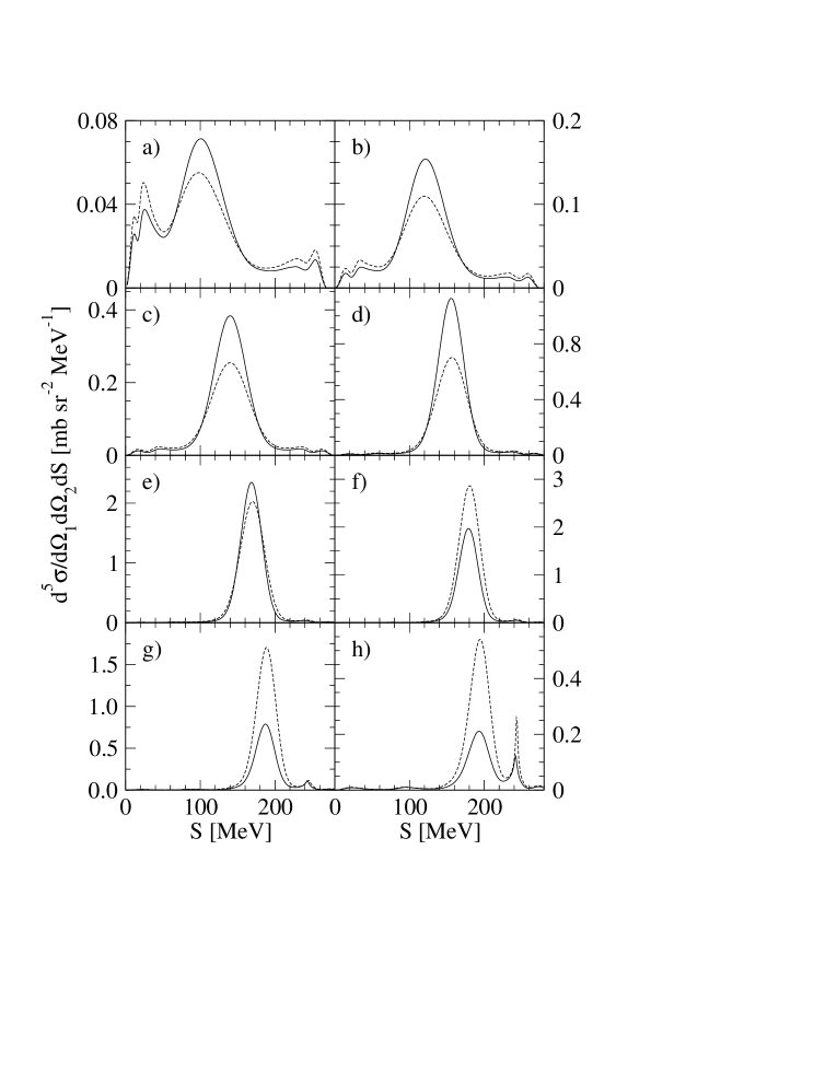
Figure 5: The five-fold cross section ${d^{5}\sigma\over{d\Omega_{1}d\Omega_{2}dS}}$ for $d(n,n_{1}n_{2})p$ breakup reaction at $E_{n}^{lab}=200$ MeV at fixed $\theta_{2}=37.5^{\circ}$, $\phi_{12}=180^{\circ}$ and varying $\theta_{1}$: a) $\theta_{1}=27.5^{\circ}$, b) $\theta_{1}=32.5^{\circ}$, c) $\theta_{1}=37.5^{\circ}$, d) $\theta_{1}=42.5^{\circ}$, e) $\theta_{1}=47.5^{\circ}$, f) $\theta_{1}=52.5^{\circ}$, g) $\theta_{1}=57.5^{\circ}$, h) $\theta_{1}=62.5^{\circ}$. The nonrelativistic and relativistic cross sections are shown by dashed and solid lines, respectively. The calculations are based on the CD Bonn potential (see text).

Results of applying that procedure are shown in the first row of Figs. 1-2 for $E_{n}^{lab}=65$ MeV and of Figs. 3-4 for $200$ MeV, separately for positive (Figs. 1 and 3) and negative (Figs. 2 and 4) values of $\Delta$. Distinguishing between positive and negative $\Delta$’s allows us to locate regions of breakup phase-space where relativity increases or diminishes the nonrelativistic cross section. Our numbers are based on the CD Bonn potential. Since we use only gray tones we split the variation of the quantity $\Delta$ into four groups. Based on the meaning of the gray tones and using the first row of Figs. 1-4 one can proceed as follows. Choosing a region in the $\theta_{1}-\theta_{2}$ plane with a black tone we know that in the $\theta_{1}-\phi_{12}$ plane there must exist also black region for the same $\theta_{1}$. This allows to read off a certain value of $\phi_{12}$. Then the angular positions of the two detectors are fixed, which defines the S-curve in the $E_{1}-E_{2}$ plane. Along such an S-curve there must be again a black region, where one can read off the corresponding range of energies. Choosing for instance another combination of tones, like a black one in the $\theta_{1}-\theta_{2}$ plane, white one in the $\theta_{1}-\phi_{12}$ plane one knows that the S-curve in the $E_{1}-E_{2}$ plane lies in the white and maybe gray regions. This should explain the use of first row from Figs. 1-4. It is seen that relativity can act in both directions, increasing or decreasing the nonrelativistic cross section. The magnitude of relativistic effects increases with energy of the incoming neutron. Whereas at $65$ MeV they approach $\approx 14\%$ when relativity increases the nonrelativistic cross section and $\approx 25\%$ in the opposite case, at $200$ MeV the corresponding numbers are $\approx 55\%$ and $\approx 60\%$, respectively. The effects are distributed over the entire phase-space. It is seen in Figs. 1-4 that at both energies (however, at $200$ MeV more clearly) the large relativistic effects have a tendency to localize in phase-space regions with small value of the undetected proton energy and when momenta of the two neutrons are coplanar on opposite sides of the beam ($\phi_{12}\approx 180^{\circ}$). Those geometries are around a region of quasi-free-scattering (QFS) condition, where the undetected proton is exactly at rest in the lab. system. When relativity increases the nonrelativistic cross section ($\Delta>0$) large relativistic effects occur at positions of detectors $\theta_{1}$ and $\theta_{2}$ around $\theta_{1}+\theta_{2}\approx 75^{\circ}$. For $\Delta<0$ this region is shifted to $\theta_{1}+\theta_{2}\approx 100^{\circ}$ leading to the following pattern of the nonrelativistic cross section variation due to relativity. Starting e.g. at fixed $\theta_{2}$ from configuration where relativity increases the nonrelativistic cross section and increasing $\theta_{1}$ we are led to configurations with decreasing $\Delta$, resulting finally in geometries where relativity diminishes the nonrelativistic cross section. In Fig. 5 we show this pattern at $200$ MeV for a number of configurations along S-curve for a fixed angle $\theta_{2}$ and changing $\theta_{1}$. Of course the same is true when exchanging $\theta_{1}$ and $\theta_{2}$. This characteristic pattern can be looked for in experimental data.

In order to get insight into the origin of maximal deviations we show in the second and the third rows of Figs. 1-4 the values of $\Delta$ calculated from the dynamical and kinematical factor of the cross section, respectively. This is done only for configurations from the first row in those figures (geometries with maximal changes of nonrelativistic cross section by relativity). It is clearly seen that the effect is predominantly due to the dynamical change of the transition matrix element. For localized phase-space regions of the large $\Delta$ values mentioned above the nonrelativistic and relativistic kinematical factors are comparable.

IV.2 Comparison to exclusive breakup cross section data

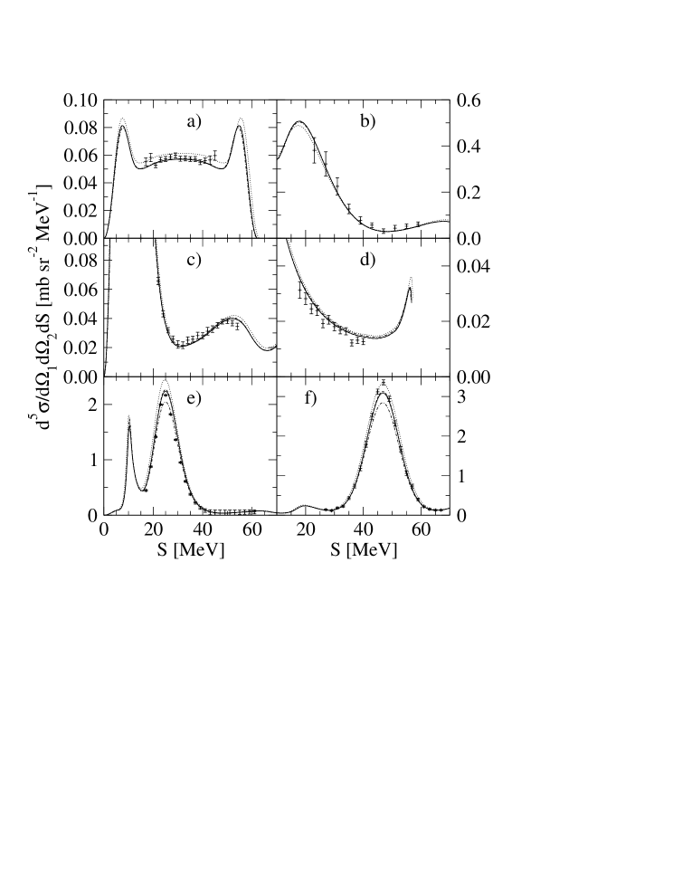
Figure 6: The five-fold cross section ${d^{5}\sigma\over{d\Omega_{1}d\Omega_{2}dS}}$ for $d(n,n_{1}n_{2})p$ breakup reaction at $E_{n}^{lab}=65$ MeV for the following positions of outgoing neutron detectors: a) $\theta_{1}=\theta_{2}=54^{\circ}$, $\phi_{12}=120^{\circ}$, b) $\theta_{1}=20^{\circ}$, $\theta_{2}=45^{\circ}$, $\phi_{12}=180^{\circ}$, c) $\theta_{1}=20^{\circ}$, $\theta_{2}=75.6^{\circ}$, $\phi_{12}=180^{\circ}$, d) $\theta_{1}=20^{\circ}$, $\theta_{2}=116.2^{\circ}$, $\phi_{12}=0^{\circ}$, e) $\theta_{1}=30^{\circ}$, $\theta_{2}=59.5^{\circ}$, $\phi_{12}=180^{\circ}$, f) $\theta_{1}=\theta_{2}=44^{\circ}$, $\phi_{12}=180^{\circ}$. The nonrelativistic and relativistic (full boost) cross sections are shown by dotted and solid lines, respectively. Neglecting the boost totally leads to dashed-dotted line. When boost is approximated by Eq.(18) results in dashed line. All calculations are based on the CD Bonn potential (see text). The $d(p,pp)n$ data are from:  zejma1997 a) ;  bodek2001a b), c) and d) ;  allet1996 e) and f).

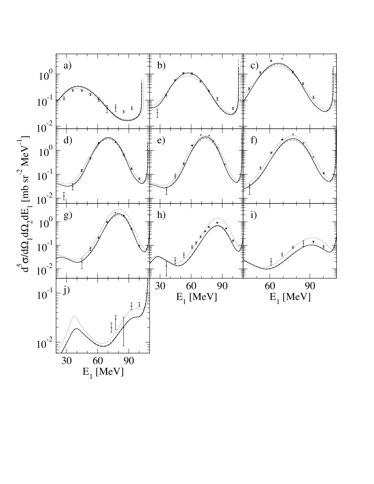
Figure 7: The five-fold cross section ${d^{5}\sigma\over{d\Omega_{1}d\Omega_{2}dE_{1}}}$ for $d(n,nn)p$ breakup reaction at $E_{n}^{lab}=156$ MeV at fixed position $\theta_{1}=45^{\circ}$, $\phi_{12}=180^{\circ}$, and varying $\theta_{2}$: a) $\theta_{2}=25^{\circ}$, b) $\theta_{2}=32.5^{\circ}$, c) $\theta_{2}=37.5^{\circ}$, d) $\theta_{2}=40^{\circ}$, e) $\theta_{2}=42.5^{\circ}$, f) $\theta_{2}=45^{\circ}$, g) $\theta_{2}=47.5^{\circ}$, h) $\theta_{2}=52.5^{\circ}$, i) $\theta_{2}=60^{\circ}$, j) $\theta_{2}=67.5^{\circ}$. Curves as in Fig.6. The $d(p,pp)n$ data are from br156 .

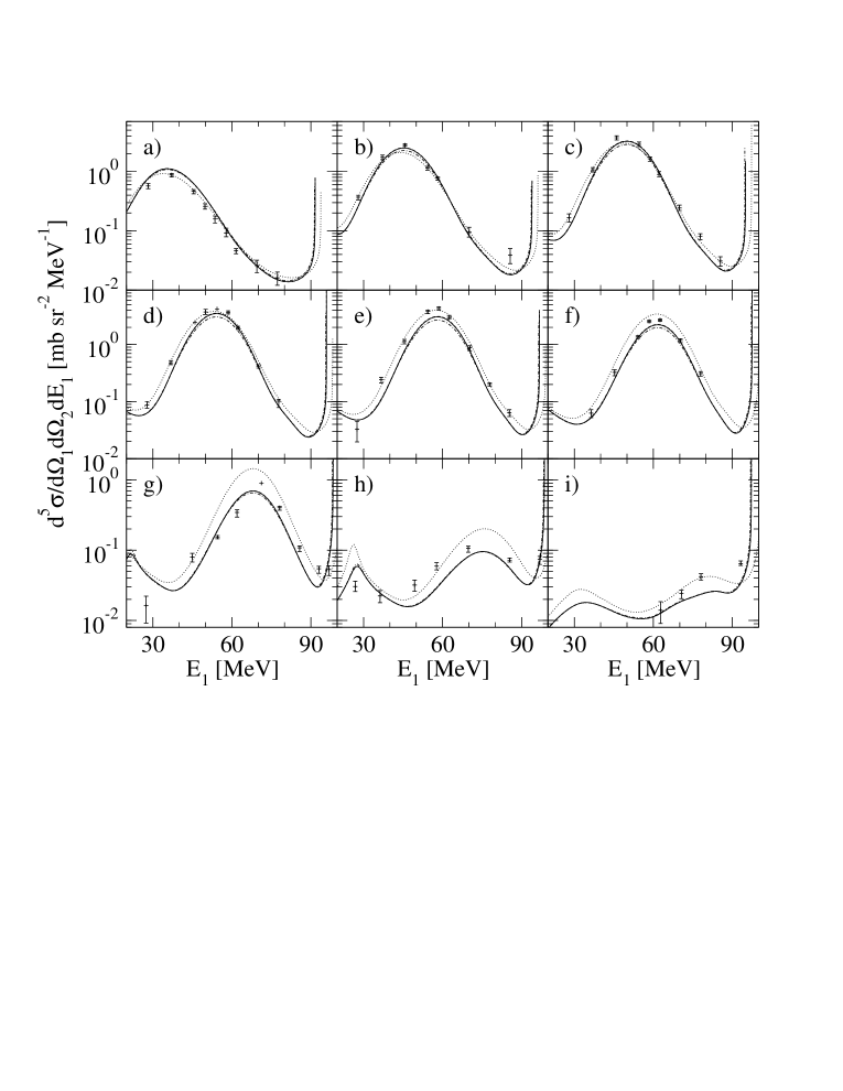
Figure 8: The same as in Fig.7 but at fixed position $\theta_{1}=52.5^{\circ}$, $\phi_{12}=180^{\circ}$, and varying $\theta_{2}$: a) $\theta_{2}=25^{\circ}$, b) $\theta_{2}=30^{\circ}$, c) $\theta_{2}=32.5^{\circ}$, d) $\theta_{2}=35^{\circ}$, e) $\theta_{2}=37.5^{\circ}$, f) $\theta_{2}=40^{\circ}$, g) $\theta_{2}=45^{\circ}$, h) $\theta_{2}=52.5^{\circ}$, i) $\theta_{2}=60^{\circ}$.

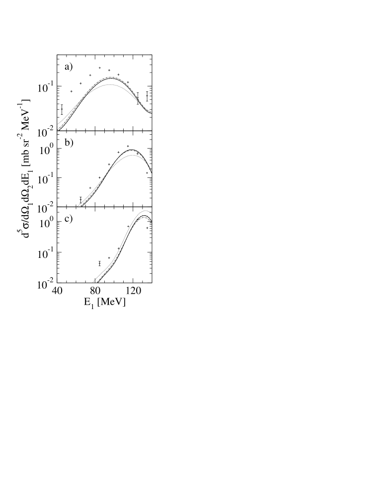
Figure 9: The five-fold cross section ${d^{5}\sigma\over{d\Omega_{1}d\Omega_{2}dE_{1}}}$ for $d(n,np)n$ breakup reaction at $E_{n}^{lab}=200$ MeV at fixed position $\theta_{1}=35^{\circ}$, $\phi_{12}=180^{\circ}$, and varying $\theta_{2}$: a) $\theta_{2}=35^{\circ}$, b) $\theta_{2}=45^{\circ}$, c) $\theta_{2}=55^{\circ}$. Curves as in Fig.6. The $d(p,pn)p$ data are from br200 .

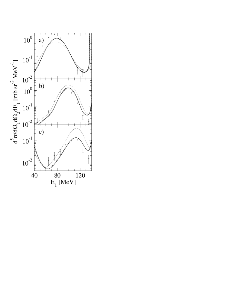
Figure 10: The same as in Fig.9 but at fixed position $\theta_{1}=45^{\circ}$, $\phi_{12}=180^{\circ}$, and varying $\theta_{2}$: a) $\theta_{2}=35^{\circ}$, b) $\theta_{2}=45^{\circ}$, c) $\theta_{2}=55^{\circ}$.

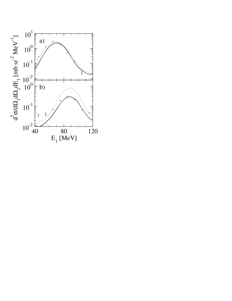
Figure 11: The same as in Fig.9 but at fixed position $\theta_{1}=52^{\circ}$, $\phi_{12}=180^{\circ}$, and varying $\theta_{2}$: a) $\theta_{2}=35^{\circ}$, b) $\theta_{2}=45^{\circ}$.

At higher energies the exclusive breakup cross sections have been measured below the pion production threshold at $65$ MeV allet1994 ; allet1996 ; zejma1997 ; bodek1998 ; bodek2001a ; kist2003b ; kist2005a , $156$ MeV br156 , and $200$ MeV br200 . In Figs. 6-11 we compare our predictions with the data taken at those energies for some complete geometries. In order to investigate importance of the boost we show for each geometry the nonrelativistic cross section (dotted line) together with three relativistic cross sections corresponding to different treatment of the boost. The first result is based on our most extensive approach to the boosted potential (approximation of Eq. (16): solid line), in the second the boost of the potential from the 2N c.m. to the 3N c.m. is totally neglected (approximation of Eq. (17): dashed-dotted line), and in the third the k-dependence of the first order relativistic boost correction is omitted (approximation of Eq. (18): dashed line).

For all presented configurations relativistic effects are clearly visible. Cases of increasing as well as diminishing the nonrelativistic cross section by relativity are represented. At $65$ MeV (see Fig.6) the smallest effects are for configurations b), c), and d) where both nonrelativistic and relativistic predictions provide a satisfactory description of data. The largest effects are for two QFS configurations e) and f), where the inclusion of relativity reduces the cross section by $\approx 9\%$, and for the symmetrical space star (SSS) configuration a) where this effect amounts to $\approx 7\%$. The SSS geometry corresponds to the situation where for the arc-length $S\approx 30$ MeV all three nucleons have equal momenta which in the 3N c.m. system lie in the plane perpendicular to the beam direction. Despite its smallness that relativistic effect leads to a better description of data for those three configurations than the nonrelativistic result. It seems to explain the small and up to now puzzling overestimation of the $65$ MeV SSS cross section data zejma1997 by modern nuclear forces and can account for the experimental width of these QFS peaks allet1994 . For QFS configurations e) and f) the boost effect is significant in the region of QFS peak. Neglecting boost decreases the relativistic cross section by $\approx 8\%$. However, approximating boost by Eq.(18) leads practically to the same result as for the full boost.

At $156$ MeV (see Figs.7 and 8) the relativistic effects are significantly larger than at $65$ MeV. Here among configurations shown there are cases where relativity increases the nonrelativistic cross section by up to $\approx 30\%$ and cases with diminished cross section by up to $\approx 50\%$. For those configurations there are regions of kinetic energies $E_{1}$ where relativity improves the description of data. One can even argue, that the pattern described in subsection IV.1 is supported by some of the presented data. Similarly to the situation at $65$ MeV importance of the boost depends on configuration and neglecting it changes the relativistic cross section up to $\approx 15\%$. It seems that the restriction to the approximation of Eq.(18) also here is sufficient for the boost treatment.

The largest relativistic effects are seen at $200$ MeV (see Figs.9-11). They can lead to changes of the nonrelativistic cross section increasing it even by up to $\approx 40\%$ or decreasing it by up to $\approx 60\%$, leading predominantly to a better description of data, which ,however , is not satisfactory in all configurations. Importance of the boost is similar to that at $156$ MeV. Also here the pattern described in subsection IV.1 is discernible. The data of ref. br200 shown in Figs.9-11 seem to be shifted in energy $E_{1}$ with respect to both nonrelativistic and relativistic predictions. Independent measurement providing cross sections with smaller error bars on the slope would be desirable.

V Summary and outlook

We numerically solved the 3N Faddeev equation for nd scattering including relativistic features such as the relativistic form of the free propagator and the change of the NN potential caused by the boost of the 2N subsystem. The calculations have been performed at the neutron lab. kinetic energies $E_{n}^{lab}=65$ MeV, $156$ MeV, and $200$ MeV. To construct the 3N momentum space basis we used the relative momentum of two nucleons in their 2N c.m. subsystem together with momentum of the spectator nucleon in the 3N c.m. system. Such a choice of momenta is adequate for relativistic kinematics and allows to generalize the nonrelativistic approach used to solve the nonrelativistic 3N Faddeev equation to the relativistic case in a more or less straightforward manner. That relative momentum in the two-nucleon subsystem is a generalisation of the standard nonrelativistic Jacobi momentum $\vec{p}$. We neglected the Wigner rotations of the nucleons spins when boosting the 2N c.m. subsystem to the 3N c.m. frame. As dynamical input we took the nonrelativistic NN potential CD Bonn and generated in the 2N c.m. system an exactly on-shell equivalent relativistic interaction $v$ using the analytical scale transformation of momenta. We checked that in our energy range the boost effects for this potential could be sufficiently well incorporated by restricting the exact expression to the leading order terms in a $q/\omega$ and $v/\omega$ expansion. At $65$ MeV and $200$ MeV we performed search for magnitudes and signs of relativistic effects on the exclusive nd breakup cross sections over the relevant parts of the breakup phase-space. We found, that depending on the phase-space region relativity can decrease as well as increase the nonrelativistic cross section. The magnitude of effects rises with the incoming neutron energy. While at $65$ MeV the effects are rather moderate ($\approx 20\%$) at $200$ MeV they can change the nonrelativistic cross section even by a factor of $\approx 2$. At that energy relativity leads to a characteristic pattern of the cross section variation with $\theta_{1}$ and $\theta_{2}$. Comparison to existing data seems to support this finding. At $65$ MeV the inclusion of relativity can explain some discrepancies found in the past between theory and data.

The selectivity of the nd breakup reaction provides opportunity to study different aspects of the 3N dynamics. Since higher energies seem to be more favorable to study properties of three-nucleon forces, precise higher energy exclusive breakup cross sections should be used as a very valuable tool to test stringently the incorporation of relativity. Especially, the configurations around the QFS breakup geometry due to their large cross sections and insensitivity to the details of nuclear forces seems to be favored for this purpose.

Figure 1: (Color online) The regions of the d(n,nn)p breakup phase-space at incoming neutron energy $E_{n}^{lab}=65$ MeV projected onto the $\theta_{1}-\theta_{2}$, $\theta_{1}-\phi_{12}$, and $E_{1}-E_{2}$ plains, carrying certain values of $\Delta$ from Eq.(39) as indicated in the boxes. In the first row the largest positive values of $\Delta$, which measure the largest increasing relativistic effect in the five-fold breakup cross section ${d^{5}\sigma\over{d\Omega_{1}d\Omega_{2}dS}}$, are shown based on the CD Bonn potential. The second and the third row shows the values of $\Delta$ obtained only with the dynamical and kinematical parts of the cross section, respectively, for configurations from the first row. The white area belongs either to phase-space regions not allowed kinematicaly or to regions rejected by our cuts on the cross sections or energies (see text).

Figure 2: (Color online) The same as in Fig. 1 but for the largest negative values of $\Delta$ at $E_{n}^{lab}=65$ MeV shown in the first row (the largest decreasing relativistic effect).

Figure 3: (Color online) The same as in Fig. 1 but for $E_{n}^{lab}=200$ MeV.

Figure 4: (Color online) The same as in Fig. 2 but for $E_{n}^{lab}=200$ MeV.

References

- (1) R.B. Wiringa, V.G.J. Stoks, R. Schiavilla, Phys. Rev. C51, 38 (1995).
- (2) R. Machleidt, F. Sammarruca, and Y. Song, Phys. Rev. C53, R1483 (1996).
- (3) V.G.J. Stoks, R.A.M. Klomp, C.P.F. Terheggen, J.J. de Swart, Phys. Rev. C49, 2950 (1994).
- (4) W. Glöckle, H.Witała, D.Hüber, H.Kamada, J.Golak, Phys.Rep. 274, 107 (1996).
- (5) H. Witała, W. Glöckle, D. Hüber, J. Golak, and H. Kamada, Phys. Rev. Lett. 81, 1183 (1998).
- (6) K. Sekiguchi et al., Phys. Rev. C65, 034003 (2002).
- (7) H. Witała, W. Glöckle, J. Golak, A. Nogga, H. Kamada, R. Skibiński, and J. Kuroś-Żołnierczuk, et al., Phys. Rev. C63, 024007 (2001).
- (8) W.P. Abfalterer et al., Phys. Rev. Lett. 81, 57 (1998).
- (9) H. Witała, H. Kamada, A. Nogga, W. Glöckle, Ch. Elster, and D. Hüber, Phys. Rev. C59, 3035 (1999).
- (10) K. Hatanaka et al., Phys. Rev. C66, 044002 (2002).
- (11) R.V. Cadman et al., Phys. Rev. Lett. 86, 967 (2001).
- (12) R. Bieber et al., Phys. Rev. Lett. 84, 606 (2000).
- (13) K. Ermisch et al., Phys. Rev. Lett. 86, 5862 (2001).
- (14) K. Ermisch et al., Phys. Rev. C68, 051001(R) (2003).
- (15) K. Ermisch et al., Phys. Rev. C71, 064004 (2005).
- (16) H. Witała, J. Golak, W. Glöckle, H. Kamada, Phys. Rev. C71, 054001 (2005).
- (17) H. Kamada, W. Glöckle, J. Golak, and Ch. Elster, Phys. Rev. C66, 044010 (2002).
- (18) H. Kamada, W. Glöckle, Phys. Rev. Lett. 80, 2547 (1998).
- (19) H. Witała, J. Golak, R. Skibiński, Phys. Lett. B634, 374 (2006).
- (20) H.Witała, T.Cornelius and W.Glöckle, Few-Body Syst. 3, 123 (1988).
- (21) W. Glöckle, T-S. H. Lee, and F. Coester, Phys. Rev. C33, 709 (1986).
- (22) F. Coester, Helv. Phys. Acta 38, 7 (1965).
- (23) W.Glöckle, The Quantum Mechanical Few-Body Problem, Springer-Verlag 1983.
- (24) M.Allet et al., Phys. Rev. C50, 602 (1994).
- (25) M.Allet et al., Few-Body Systems 20, 27 (1996).
- (26) J. Zejma et al, Phys. Rev. C55, 42 (1997).
- (27) K. Bodek et al., Nucl. Phys. A631, 687c (1998).
- (28) K. Bodek et al., Few-Body Systems 30, 65 (2001).
- (29) St. Kistryn et al., Phys. Rev. C68, 054004 (2003).
- (30) St. Kistryn et al., Phys. Rev. C72, 044006 (2005).
- (31) F. Takeutchi, T. Yuasa, K. Kuroda, and Y. Sakamoto, Nucl. Phys. A152, 434 (1970).
- (32) W. Pairsuwan, J.W. Watson, M. Ahmad, N.S. Chant, B.S. Flanders, R. Madey, P.J. Pella, and P.G. Roos, Phys. Rev. C52, 2552 (1995).