Diagrammatic calculation of thermodynamical quantities in nuclear matter

Abstract

In medium $T-$matrix calculations for symmetric nuclear matter at zero and finite temperatures are presented. The internal energy is calculated from the Galitskii-Koltun’s sum rule and from the summation of the diagrams for the interaction energy. The pressure at finite temperature is obtained from the generating functional form of the thermodynamic potential. The entropy at high temperature is estimated and compared to expressions corresponding to a quasiparticle gas.

I Introduction

The description of nuclear matter and its thermodynamic properties is an important issue for the modeling of hot neutron stars and intermediate energy heavy-ion collisions. A possible approach consists in trying to calculate the bulk properties of the many-body system, starting from a free N-N potential. Strong N-N interactions induce short range correlations in nuclear matter, which have to be treated consistently in the dense system. The effect of the short range interactions on the binding energy depends on the particular free N-N potential used; moreover it is known that, in order to reproduce the empirical saturation point in symmetric nuclear matter, three-body forces must be considered. In the present paper we present a study restricted to a model using the two-body CD-Bonn potential only, while three-body interactions will be included in a further publication.

A thermodynamically consistent approximation which resums the short range correlations can be constructed from a suitably chosen generating functional Baym and Kadanoff (1961); Baym (1962). For nuclear interactions the generating functional must at least include the sum of ladder type diagrams, this choice leads to the in medium $T-$matrix approximation Baym and Kadanoff (1961). This is the approximation scheme adopted in our study. At zero temperature it yields results for binding energy, pressure, and single particle-energy compatible with each other Bożek and Czerski (2001); Bożek (2002a). Thermodynamical relations are fulfilled, including the celebrated Hugenholz-Van Hove and Luttinger identities Hugenholz and Hove (1958); Luttinger (1960). The thermodynamically consistent in-medium $T-$matrix approach at zero temperature Bożek and Czerski (2003, 2002); Dewulf et al. (2002, 2003) yields results for the binding energy similar to extensive variational and Brueckner-Hartree-Fock approaches Akmal et al. (1998); Wiringa et al. (1988); Baldo and Burgio (2001); Baldo et al. (2002).

Much less studies are available at finite temperatures. Some nuclear matter calculations at finite temperature within the Brueckner-Hartree-Fock approach have been performed Baldo and Ferreira (1998); Zuo et al. (2006). The in medium $T-$matrix scheme based on finite-temperatures Green’s functions can be easily applied to calculate the internal energy or the single-particle properties Bożek (1999a, 2002b); Frick and Müther (2003); Frick et al. (2004, 2005), however no estimates for the pressure or the entropy of the interacting nucleon system with short range correlations are available within this approach. At zero temperature the pressure $P$ can be calculated from the binding energy per particle $E/N$ using the thermodynamic relations $P=\rho(\mu-E/N)$ or $P=\rho^{2}\frac{\partial(E/N)}{\partial\rho}$, where $\rho$ is the nuclear matter density and $\mu$ is the chemical potential Bożek and Czerski (2001). In principle, the thermodynamic identities

$$\left(\frac{\partial PV}{\partial T}\right)_{\mu,V}=\frac{E+PV-\mu N}{T}\ \ ;\ \ T\left(\frac{\partial S}{\partial T}\right)_{\mu,V}=\left(\frac{\partial(E-\mu N)}{\partial T}\right)_{\mu,V}$$ (1)

could be integrated in order to obtain the pressure or the entropy $S$ at non-zero temperatures ($V$ is the volume of the system). In practice, the above equations cannot be employed to estimate numerically the pressure since an inaccurate evaluation of the numerators yields uncontrollable errors for the entropy at small temperatures. The pressure can be calculated instead from the diagrammatic expansion of the thermodynamic potential. Through the relation

$$TS=E+PV-\mu N\ \>$$ (2)

the entropy can be reliably estimated for sufficiently large temperatures. In section II we discuss diagrammatic procedures for calculating the energy of the system and compare the result to the Galitskii-Koltun’s formula. By varying the strength of the interaction potential in the diagrammatic formula for the internal energy we obtain an expression for the pressure of the interacting system (section III). The entropy is also estimated and compared with a reduced formula and with the result for a free gas of Fermions with in-medium modified masses.

II Energy of the interacting system

The (total) internal energy per particle can be calculated as the expectation value of the Hamiltonian of the system $H=H_{kin}+H_{pot}$

$$\frac{E}{N}=\frac{1}{\rho}\left[\frac{\langle H_{kin}\rangle}{V}+\frac{\langle H_{pot}\rangle}{V}\right]\>.$$ (3)

When we evaluate the right hand side of (3) in momentum space we see that the kinetic part is

$$\langle H_{kin}\rangle=V\int\frac{d^{3}{p}}{(2\pi)^{3}}\frac{d\omega}{2\pi}\frac{\mathbf{p}^{2}}{2m}A(\mathbf{p},\omega)f(\omega)\>,$$ (4)

while the potential term takes the form

$$\langle H_{pot}\rangle=\displaystyle\frac{V}{2}\int\frac{d^{3}P}{(2\pi)^{3}}\frac{d^{3}{k}}{(2\pi)^{3}}\frac{d^{3}{k^{\prime}}}{(2\pi)^{3}}\frac{d\Omega}{2\pi}V(\mathbf{k},\mathbf{k^{\prime}})\langle\mathbf{k^{\prime}}|G_{2}^{<}(\mathbf{P},\Omega)|\mathbf{k}\rangle\ .$$ (5)

Here $A(\mathbf{p},\omega)$ is the spectral function, $f(\omega)$ is the Fermi distribution and $V(\mathbf{k},\mathbf{k^{\prime}})$ the interaction potential (we skip the spin and isospin indices in the notation). $\langle\mathbf{k^{\prime}}|G_{2}^{<}(\mathbf{P},\Omega)|\mathbf{k}\rangle$ is the two particle Green’s function with a common time for the incoming lines and a common time for the outgoing lines. The outgoing time is set to be larger than the incoming time (this corresponds to ^< ordering on the real-time contour) Keldysh (1964); Danielewicz (1984); after integration over the total energy of the pair $\Omega$, the incoming and outgoing times are set to the same value. The presence of the full two-particle propagator requires the use of diagrammatic calculation techniques, in particular the two-particle Green’s function must be calculated within the chosen approximation scheme. Alternatively, it is possible to determine the total energy in a simpler way through the Galitskii-Koltun’s sum rule Galitskii and Migdal (1958); Martin and Schwinger (1959); Koltun (1972)

$$\frac{E}{N}=\frac{1}{\rho}\int\frac{d^{3}{p}}{(2\pi)^{3}}\frac{d\omega}{2\pi}\left[\frac{\mathbf{p}^{2}}{2m}+\omega\right]A(\mathbf{p},\omega)f(\omega)\>.$$ (6)

For conserving approximations, as well as in case when the full (exact) solutions for the two-particle Green’s function and the spectral function are used, the expression for the energy of the system in the form of the above sum rule is equivalent to the direct calculation (3). On the other hand this does not remain valid when three-body forces are included: in that case the Galitskii-Koltun’s sum rule cannot be employed and the energy has to be evaluated directly from the expectation value of the Hamiltonian.

Let us first note that the simplest way of approximating a two-particle Green’s function consists in constructing a product of two single one-body propagators $G$. We shall call this simple approximation non correlated two-particle Green’s function and indicate it with $G_{2}^{nc}$ (we restrict our formulas to the case when the times of the two incoming as well as the two outgoing lines are the same):

$$\langle\mathbf{k^{\prime}}|{G_{2}^{nc\ <(>)}}(\mathbf{P},\Omega)|\mathbf{k}\rangle=$$

$$=\displaystyle i(2\pi)^{3}\delta(\mathbf{k}-\mathbf{k^{\prime}})\int\frac{d\omega^{\prime}}{2\pi}G^{<(>)}(\mathbf{P}/2+\mathbf{k},\Omega-\omega^{\prime})G^{<(>)}(\mathbf{P}/2-\mathbf{k},\omega^{\prime})\>.$$ (7)

The single-particle Green’s function $G$ denotes the in-medium dressed propagator, which includes the self-energy resummed in the chosen approximation. In the self-consistent $T-$matrix approximation the dressed propagator involves a nontrivial dispersive self-energy which leads to a broad spectral function Bożek (2002b). We then introduce the in-medium two-particle scattering matrix $T$, defined by

$$\langle\mathbf{k}|T^{R(A)}(\mathbf{P},\Omega)|\mathbf{k^{\prime}}\rangle=V(\mathbf{k},\mathbf{k^{\prime}})$$

$$+\displaystyle\int\frac{d^{3}{p}}{(2\pi)^{3}}\frac{d^{3}{q}}{(2\pi)^{3}}V(\mathbf{k},\mathbf{p})\langle\mathbf{p}|{G_{2}^{nc\ R(A)}}(\mathbf{P},\Omega)|\mathbf{q}\rangle\langle\mathbf{q}|T^{R(A)}(\mathbf{P},\Omega)|\mathbf{k^{\prime}}\rangle\>,$$ (8)

where we have used the non correlated two-particle Green’s function defined above, with the time ordering in the times of the incoming and outgoing lines changed to the retarded $G_{2}^{R}$ or advanced $G_{2}^{A}$ one (the same time ordering is chosen for the $T-$matrix) Danielewicz (1984). The self-consistent $T-$matrix approach is an iterative scheme involving the calculation of the $T-$matrix, the calculation of the self-energy Bożek (1999a)

$$\mbox{Im}\Sigma(\mathbf{p},\omega) = \int\frac{d^{3}{k}}{(2\pi)^{3}}\frac{d{\omega^{{}^{\prime}}}}{2\pi}\left[\mbox{Im}\langle(\mathbf{p-k})/2|T^{R}(\mathbf{p+k},\Omega)|(\mathbf{p-k})/2\rangle-\right.$$ (9)

$$\left.\mbox{Im}\langle(\mathbf{p-k})/2|T^{R}(\mathbf{p+k},\Omega)|(\mathbf{k-p})/2\rangle\right]\left[b(\omega+\omega^{{}^{\prime}})+f(\omega^{{}^{\prime}})\right]A(\mathbf{k},\omega^{{}^{\prime}})$$

and of the Dyson equation

$$G^{R(A)\ -1}(\mathbf{p},\omega)=\omega-\frac{p^{2}}{2m}-\Sigma^{R(A)}(\mathbf{p},\omega)\ .$$ (10)

The $T-$matrix approximation can be as well obtained from a generating functional $\Phi[G,V]$ which is a set of two-particle irreducible diagrams Baym (1962) obtained by closing two-particle ladder diagrams with a combinatorial factor $1/2n$, where $n$ is the number of interaction lines in the diagram.

Figure 1: Two-particle irreducible functional for the $T-$matrix approximation. The sum runs over the number of interaction lines $n$ in the two-particle ladders.

The functional $\Phi$ depends on the dressed propagators (lines in Fig. 1) and on the two-particle potential (wavy lines in Fig. 1). The self-energy is then given as a functional derivative $\displaystyle\Sigma=\frac{\delta\Phi}{\delta G}$.

An approximation for $G_{2}$, which we shall indicate with the italic character $\mathcal{G}_{2}$, can be written as follows

$$\langle\mathbf{k}|\mathcal{G}_{2}^{R(A)}(\mathbf{P},\Omega)|\mathbf{k^{\prime}}\rangle=\langle\mathbf{k}|{G_{2}^{nc\ R(A)}}(\mathbf{P},\Omega)|\mathbf{k^{\prime}}\rangle-\langle\mathbf{k}|{G_{2}^{nc\ R(A)}}(\mathbf{P},\Omega)|\mathbf{-k^{\prime}}\rangle$$

$$+\displaystyle\int\frac{d^{3}{p}}{(2\pi)^{3}}\frac{d^{3}{q}}{(2\pi)^{3}}\left\{\langle\mathbf{k}|{G_{2}^{nc\ R(A)}}(\mathbf{P},\Omega)|\mathbf{p}\rangle-\langle\mathbf{k}|{G_{2}^{nc\ R(A)}}(\mathbf{P},\Omega)|\mathbf{-p}\rangle\right\}$$

$$\times\displaystyle\langle\mathbf{p}|T^{R(A)}(\mathbf{P},\Omega)|\mathbf{q}\rangle\langle\mathbf{q}|{G_{2}^{nc\ R(A)}}(\mathbf{P},\Omega)|\mathbf{k^{\prime}}\rangle\>.$$ (11)

We insert this expression in (5) and we get

$$\langle H_{pot}\rangle = \frac{V}{2}\int\frac{d^{3}{P}}{(2\pi)^{3}}\frac{d^{3}{k}}{(2\pi)^{3}}\frac{d\Omega}{2\pi}\left[\langle\mathbf{k}|T(\mathbf{P},\Omega)|\mathbf{k}\rangle\right.$$ (12)

$$\left.\times\left(\langle\mathbf{k}|{G_{2}^{nc}}(\mathbf{P},\Omega)|\mathbf{k}\rangle-\langle\mathbf{k}|{G_{2}^{nc}}(\mathbf{P},\Omega)|\mathbf{-k}\rangle\right)\right]^{<}\>,$$

where the superscript ^< concerns the time ordering of the product $T\ G_{2}^{nc}$.

Figure 2: Diagrammatic expression for the expectation value of the potential energy. As in Fig. 1, the sum runs over the number of interaction lines $n$ in the diagram.

Figure 3: The internal energy per particle at zero temperature as a function of the density (in units of the empirical saturation density $\rho_{0}=0.16$ fm^-3). The solid line represents the expectation value of the Hamiltonian (3) and the dashed line is the result obtained from the Galitskii-Koltun’s sum rule (6).

Finally, the explicit formula with the retarded functions is

$$\langle H_{pot}\rangle=\frac{V}{2}\int\frac{d^{3}{P}}{(2\pi)^{3}}\frac{d^{3}{k}}{(2\pi)^{3}}\frac{d\Omega}{2\pi}\,b(\Omega)\,\displaystyle\mbox{Im}\left\{\left(\langle\mathbf{k}|T^{R}(\mathbf{P},\Omega)|\mathbf{k}\rangle-\langle\mathbf{k}|T^{R}(\mathbf{P},\Omega)|\mathbf{-k}\rangle\right)\,{G_{2}^{nc\ R}}(\mathbf{P},\mathbf{k},\Omega)\right\}\>,$$ (13)

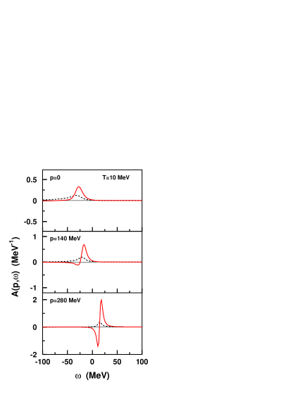
where $b(\Omega)$ is the Bose-Einstein distribution (Fig. 2). The same expression can be obtained equivalently in the imaginary time formalism.

We calculate the internal energy per particle with the use of the two methods:

1. from the Galitskii-Koltun’s sum rule (6);

2. from diagram summation, i.e. from eq. (3) together with (4) and (13).

Results for the symmetric nuclear matter at zero temperature with the CD Bonn potential are displayed in Fig. 3. The calculation are performed using a numerical procedure where the energy range is limited to an interval $[-\omega_{c},\omega_{c}]$. We have tested several values of the energy scale $\omega_{c}$ between $2\,\mbox{GeV}$ and $10\,\mbox{GeV}$, and we found that the Galitskii-Koltun’s sum rule expression for the energy shows some dependence on this value. On the other hand, the results obtained from the direct estimation of the interaction and kinetic energies are stable and independent on the energy range taken (up to an inaccuracy due to numerical discretization of about $0.5$ MeV). The result from the diagram summation can be compared to Galitskii-Koltun’s sum rule result extrapolated to infinite energy range (Fig. 3). The values obtained in two ways differ by about $0.9$ MeV at the saturation density. Besides the numerical inaccuracies another source of the difference between the internal energy from the Galitskii-Koltun’s sum rule and from the expression (3) can be attributed to the effect of the angular averaging of the two-particle propagator in the $T-$matrix calculation Schiller et al. (1999). Such a technical approximation is used in order to allow for a partial-wave expansion of the in-medium $T-$matrix. In the following we use for the internal energy either the Galitskii-Koltun’s sum rule result extrapolated to infinite energy range or the expression (3). We find differences of the same order using the two methods of calculating the internal energy also at finite temperatures (Table 1).

As stated in section I the calculation using only a two-body force are not complete, e.g. the saturation density is too large, and only the result of a study which includes three-nucleon interactions could be compared to an experimentally estimated equation of state of nuclear matter. Therefore in the following we restrict ourselves only to the empirical saturation density $\rho_{0}=0.16$ fm^-3 to illustrate the calculation of the pressure and entropy.

III Pressure and entropy

The pressure is related to the thermodynamical potential through

$$\Omega(T,\mu,V)=-PV\>.$$ (14)

It can be shown that $\Phi$ gives a contribution to the thermodynamical potential Fetter and Walecka (1971), and in particular that

$$\Omega=-\mbox{Tr}\{\ln[G^{-1}]\}-\mbox{Tr}\{\Sigma G\}+\Phi\>.$$ (15)

In the real-time formalism the trace involves the integration over energy and momenta, with the time ordering corresponding to ^<; however the equations are most easily derived in the imaginary time formalism, where the trace implies a summation over Matsubara frequencies together with an integration over momenta, and the Matsubara representation of the dressed single-particle Green’s function takes the form

$$G(\mathbf{p},i\omega_{n})=\int\frac{d\omega}{2\pi}\frac{A(\mathbf{p},\omega)}{i\omega_{n}-\omega}\ \ .$$ (16)

We write the pressure as a sum of two terms

$$P_{tot}=P_{I}+P_{II}\>,$$ (17)

where

$$P_{I}=\frac{1}{V}\left[\mbox{Tr}\{\ln[G^{-1}]\}+\mbox{Tr}\{\Sigma G\}\right]\>$$ (18)

and

$$P_{II}=-\frac{\Phi}{V}\>.$$ (19)

The two contributions in (18) give respectively

$$\displaystyle\mbox{Tr}\{\ln[G^{-1}]\} = VT\displaystyle\int\frac{d^{3}{p}}{(2\pi)^{3}}\frac{d\omega}{2\pi}\ln(1+e^{-\beta\omega})\left[A(\mathbf{p},\omega)+\right.$$ (20)

$$+ \displaystyle 2\,\frac{\partial\mbox{Re}\Sigma^{R}(\mathbf{p},\omega)}{\partial\omega}\mbox{Im}G^{R}(\mathbf{p},\omega)+2\,\frac{\partial\mbox{Im}\Sigma^{R}(\mathbf{p},\omega)}{\partial\omega}\mbox{Re}G^{R}(\mathbf{p},\omega)\left.\right]\>$$

and

$$\mbox{Tr}\{\Sigma G\} = \displaystyle VT\int\frac{d^{3}{p}}{(2\pi)^{3}}\frac{d\omega}{2\pi}\ln(1+e^{-\beta\omega})\left[\right.\frac{\partial A(\mathbf{p},\omega)}{\partial\omega}\mbox{Re}\Sigma^{R}(\mathbf{p},\omega)$$ (21)

$$+ \displaystyle A(\mathbf{p},\omega)\frac{\partial\mbox{Re}\Sigma^{R}(\mathbf{p},\omega)}{\partial\omega}-2\,\frac{\partial\mbox{Im}\Sigma^{R}(\mathbf{p},\omega)}{\partial\omega}\mbox{Re}G^{R}(\mathbf{p},\omega)$$

$$- 2\,\mbox{Im}\Sigma^{R}(\mathbf{p},\omega)\frac{\partial\mbox{Re}G^{R}(\mathbf{p},\omega)}{\partial\omega}\left.\right]\>,$$

so that

$$\displaystyle P_{I} = T\int\frac{d^{3}p}{(2\pi)^{3}}\frac{d\omega}{2\pi}\ln(1+e^{-\beta\omega})\left[\right.A(\mathbf{p},\omega)+$$ (22)

$$+ \displaystyle\frac{\partial A(\mathbf{p},\omega)}{\partial\omega}\mbox{Re}\Sigma^{R}(\mathbf{p},\omega)-2\mbox{Im}\Sigma^{R}(\mathbf{p},\omega)\frac{\partial\mbox{Re}G^{R}(\mathbf{p},\omega)}{\partial\omega}\left.\right]$$

$$= T\int\frac{d^{3}p}{(2\pi)^{3}}\frac{d\omega}{2\pi}\ln(1+e^{-\beta\omega})B(\mathbf{p},\omega)\>.$$

We introduce a new weight function $B(\mathbf{p},\omega)$ Weinhold et al. (1998); it is normalized similarly as the spectral function $A(\mathbf{p},\omega)$

$$\int\frac{d\omega}{2\pi}B(\mathbf{p},\omega)=1$$ (23)

but assumes negative as well as positive values. The spectral function at small temperature exhibits a sharp peak at momenta close to the Fermi momentum, causing difficulties in numerical calculations. In ref. Bożek (2002b) this problem was avoided by separating the spectral function into a smooth background part and an approximate $\delta$ function

$$A(\mathbf{p},\omega)=A_{bg}(\mathbf{p},\omega)+W_{p}\,2\pi\,\delta(\omega-\omega_{p})\ .$$ (24)

Figure 4: (Color online) The spectral function $A(\mathbf{p},\omega)$ (dashed line) and the function $B(\mathbf{p},\omega)$ (solid line) calculated for symmetric nuclear matter at $T=10$ MeV.

For the weight function $B(\mathbf{p},\omega)$ a similar separation is performed

$$B(\mathbf{p},\omega)=B_{bg}(\mathbf{p},\omega)+2\pi\,W_{p}\,\mbox{Re}\Sigma(\mathbf{p},\omega)\,\delta^{{}^{\prime}}(\omega-\omega_{p})+\frac{W_{p}\,\mbox{Im}\Sigma(\mathbf{p},\omega)}{(\omega-\omega_{p})^{2}}\ ,$$ (25)

which conserves the property (23).

$\;T\;$	$\;E_{GK}/N\;$	$\;E_{diag}/N\;$	$\;P_{I}/\rho\;$	$\;P_{II}/\rho\;$	$\;P_{tot}/\rho\;$	$\;P_{quasi}/\rho\;$	$\;P_{BF}/\rho\;$
$0$	$-15.80$	$-16.63$	$-40.19$	$32.50$	$-7.69$	$-0.85$	$-5.58$
$2$	$-15.15$	$-16.29$	$-38.40$	$32.54$	$-5.86$	$-0.78$	$-5.4$
$5$	$-14.40$	$-15.24$	$-37.83$	$32.35$	$-5.48$	$-0.74$	$-5.2$
$10$	$-11.15$	$-11.72$	$-34.02$	$31.36$	$-2.66$	$-0.49$	$-3.35$
$20$	$-1.29$	$-1.21$	$-24.43$	$30.92$	$\>\>6.49$	$\>\>0.17$	$4.74$

Table 1: Results (at $\rho=\rho_{0}$) of the internal energy and the pressure at zero and finite temperature (all values in MeVs) with the CD-Bonn interaction. The second and third colum represent the internal energy per particle obtained from the Galitskii-Koltun’s sum rule (6) and from the diagram summation (3). The other columns correspond to the partial results (18) and (19), to the sum (17) and to the quasiparticle expression (28) for the pressure. In the last column are quoted the results of Baldo and Ferreira Baldo and Ferreira (1998), obtained with the Argonne $v_{14}$ interaction.

The diagrams contributing to the $\Phi$ functional are summed in the following way. One notes that for the $T-$matrix approximation the expressions for the interaction energy and the functional $\Phi$ differ by the factor $1/n$ where $n$ is the number of interaction lines in the diagram (Figs. 1 and 2). In that case, the functional $\Phi$ can be obtained from the formula for the interaction energy

$$\Phi=\int_{0}^{1}\frac{d\lambda}{\lambda}<H_{pot}(\lambda V,G_{\lambda=1})>\ \ .$$ (26)

In the above formula the interaction potential is multiplied by the factor $\lambda$ but the propagator $G$ is the dressed nucleon propagator corresponding to the system with the full strength of interactions $(\lambda=1)$. The method for calculating the functional $\Phi$ that we use (26) should not be confused with the textbook expression for the pressure of an interacting system Baym (1962); Fetter and Walecka (1971)

$$PV=P_{0}V+\int_{0}^{1}\frac{d\lambda}{\lambda}<H_{pot}(\lambda V,G_{\lambda})>\ \ ,$$ (27)

where $P_{0}$ is the pressure of a noninteracting system and the average interaction $<H_{pot}>$ is calculated in a system with the potential reduced by a factor $\lambda$ and using the propagator $G_{\lambda}$ calculated self-consistently in the system with reduced interactions.

The results of the calculations, for different temperatures, are shown in table 1. We observe a steady increase of the pressure with the temperature. Only at the lowest temperatures some modifications of this behavior are visible, which may be due to changes in the single-particle properties close to the critical point for the pairing transition Alm et al. (1996); Schnell et al. (1999); Bożek (1999b, 2002c); Guttormsen et al. (2003); Dean and Hjorth-Jensen (2003). We compare our results with the pressure of a gas of quasiparticles in a mean-field potential

$$P_{qp}=\int\frac{d^{3}p}{(2\pi)^{3}}f(\omega_{p}-\mu)\left[\frac{{p}}{3}\frac{d\omega_{p}}{dp}+\frac{1}{2}\Sigma_{p}\right]\>,$$ (28)

with $\Sigma_{p}=\Sigma(p,\omega_{p})=\omega_{p}-p^{2}/2m+\mu$ . The expression (28) is the formula for the pressure in the mean-field approximation, with $\Sigma_{p}$ taken for the mean-field. The results are very different from the full calculation with dispersive self-energies and spectral functions. Hence we conclude that, using the CD-Bonn potential, the pressure cannot be obtained from the mean-field-like formula (28) around saturation density. At low densities or high temperatures the pressure in a interacting nucleon gas can be obtained in a model independent way from the elastic scattering phase shifts Beth and Uhlenbeck (1937); Pratt et al. (1987); Horowitz and Schwenk (2005). However at the saturation density (at low temperatures) the pressure cannot be reliably calculated from a viral expansion. The pressure in hot nuclear matter has been obtained using two-body Argonne $v_{14}$ interaction in the Bloch-De Dominicis approach Baldo and Ferreira (1998). The results are qualitatively similar, with a negative value of the pressure at $T=0$ and $\rho\simeq 0.16$ fm^-3. This shows the need to include three-body forces for a reliable description of the thermodynamics of the nuclear matter.

We compute the entropy through the thermodynamic relation

$$\frac{S}{N}=\frac{1}{T}\left[\frac{E}{N}+\frac{P_{tot}}{\rho}-\mu\right]\>.$$ (29)

The results are displayed in table 2.

$\;T\>\>(\mbox{MeV})\;$	$\;\;S_{GK}/N\;\;$	$\;\;S_{diag}/N\;\;$	$\;\;S_{free}/N\;\;$	$m^{\star}\>\>(\mbox{MeV})$	$\;\;S_{free^{\star}}/N\;\;$	$\;\;S_{DQ}/N\;\;$
$2$	$0.24$	$-0.37$	$0.27$	$873$	$0.24$	$0.28$
$5$	$0.53$	$0.35$	$0.66$	$853$	$0.60$	$0.58$
$10$	$1.04$	$0.98$	$1.22$	$802$	$1.07$	$1.05$
$20$	$1.76$	$1.76$	$2.02$	$745$	$1.74$	$1.70$

Table 2: Entropy per baryon. The results for the interacting system in the $T$-matrix approximation using the Galitskii-Koltun’s sum rule (6) and Eq. (3) expressions for for the internal energy are shown in columns $S_{GK}/N$ and $S_{diag}/N$ respectively. $S_{DQ}/N$ denotes the results of Rios et al. (2006) (Eq. 30). $S_{free}/N$ and $S_{free}^{\star}/N$ are the entropies per baryon in a free Fermi gas with the free and in medium masses respectively.

The error in the calculation of $TS$ at each temperature can be estimated by comparing the results obtained with the two expressions for the internal energy (3) and (6). The difference is of the order of $1$ MeV, also at zero temperature we find $|TS|\simeq 1\,\mbox{MeV}\neq 0$. The entropy can be estimated reliably only for $T\geq 5$ MeV, with the uncertainty shown as the hatched band in Fig. 5.

We compare these results with other methods of calculating the entropy:

1. The dynamical quasiparticle formula Carneiro and Pethick (1975)

   $$\frac{S_{DQ}}{N}=\frac{1}{\rho}\int\frac{d^{3}p}{(2\pi)^{3}}\frac{d\omega}{2\pi}\sigma(\omega)\left[A({\bf p},\omega)\left(1-\frac{\partial\mbox{Re}\Sigma^{R}(\mathbf{p},\omega)}{\partial\omega}\right)+\frac{\partial\mbox{Re}G^{R}(\mathbf{p},\omega)}{\partial\omega}\Gamma(\mathbf{p},\omega)\right]\ \ ,$$ (30)

   where

   $$\sigma(\omega)=-f(\omega)\ln[f(\omega)]-[1-f(\omega)]\ln[1-f(\omega)]\>.$$ (31)

   It has been shown that this one-body formula gives results close to the complete expression for the entropy Rios et al. (2006).

2. The entropy for a free Fermi gas

   $$\frac{S_{free}}{N}=\frac{1}{\rho}\int\frac{d^{3}p}{(2\pi)^{3}}\ \sigma\left(\frac{p^{2}}{2m}\right)\ \ .$$ (32)

3. The entropy calculated as for a free Fermi gas but using the effective mass $m^{*}$ instead of the rest mass $m$

   $$\frac{S_{{free}^{\star}}}{N}=\frac{1}{\rho}\int\frac{d^{3}p}{(2\pi)^{3}}\ \sigma\left(\frac{p^{2}}{2m^{\star}}\right)\ \ .$$ (33)

   The effective mass $m^{*}$ is determined at each temperature by

   $${\left(\frac{\partial{\omega}_{p}}{\partial p^{2}}\right)}_{p=p_{F}}=\frac{1}{2m^{\star}}\>.$$ (34)

Figure 5: (Color online) Entropy per baryon as a function of the temperature. The hatched band denotes our estimate of the entropy corresponding to the two values $S_{GK}$ and $S_{diag}$ from Table 2. The solid line denotes the result for the free Fermi gas with the in-medium effective mass and the dashed line represents the result of Rios et al. (2006) (Eq. 30).

Remarkably, we find that the expression for the entropy of the free Fermi gas is very similar to the result of the full calculation for the interacting system, if the change of the effective mass in the system is taken into account. The last observation simplifies significantly the modeling of the evolution of protoneutron stars Prakash et al. (1997), since relations between the entropy per baryon and the temperature derived in the case of a fermion gas can be used in hot nuclear matter. As observed in Rios et al. (2006) the quasiparticle expression (30) for the entropy Carneiro and Pethick (1975) follows closely the full result.

IV Discussion

We study the properties of nuclear matter with short range correlations at finite temperatures up to $T=20$ MeV. We calculate the internal energy, the pressure, and the entropy. It is to our knowledge the first calculation of the pressure and of the entropy in the thermodynamically consistent $T-$matrix approximation in nuclear matter. Besides the usually employed Galitskii-Koltun’s sum rule for the internal energy, we perform a summation of diagrams corresponding to the expectation value of the interaction energy. The two methods yield similar results, up to a difference of about $1$ MeV which can be attributed to numerical inaccuracies and to the angular averaging used in the partial wave expansion of the in medium $T-$matrix. The calculation of the pressure requires a summation of a different set of diagrams, due to different numerical factors. The result is most easily obtained by an integration over an artificial parameter $\lambda$ multiplying the interaction lines, while keeping the propagators dressed as in the fully correlated system. From the pressure and the internal energy we obtain the entropy per baryon at temperatures $T\geq 5$ MeV with an uncertainty that we estimate to be $1\,\mbox{MeV}/T$. The entropy of the free Fermi gas turns out to be close to the result of the full calculation if the change of the effective mass in the medium is taken into account.

References

- Baym and Kadanoff (1961) G. Baym and L. Kadanoff, Phys. Rev. 124, 287 (1961).
- Baym (1962) G. Baym, Phys. Rev. 127, 1392 (1962).
- Bożek and Czerski (2001) P. Bożek and P. Czerski, Eur. Phys. J. A11, 271 (2001), eprint [http://arXiv.org/abs]nucl-th/0102020.
- Bożek (2002a) P. Bożek, Eur. Phys. J. A15, 325 (2002a), eprint nucl-th/0204034.
- Hugenholz and Hove (1958) N. Hugenholz and L. V. Hove, Physica 24, 363 (1958).
- Luttinger (1960) J. M. Luttinger, Phys. Rev. 119, 1151 (1960).
- Bożek and Czerski (2003) P. Bożek and P. Czerski, Acta Phys. Polon. B34, 2759 (2003), eprint nucl-th/0212035.
- Bożek and Czerski (2002) P. Bożek and P. Czerski, Phys. Rev. C66, 027301 (2002), eprint nucl-th/0204012.
- Dewulf et al. (2002) Y. Dewulf, D. Van Neck, and M. Waroquier, Phys. Rev. C65, 054316 (2002).
- Dewulf et al. (2003) Y. Dewulf, W. H. Dickhoff, D. Van Neck, E. R. Stoddard, and M. Waroquier, Phys. Rev. Lett. 90, 152501 (2003), eprint nucl-th/0303047.
- Akmal et al. (1998) A. Akmal, V. R. Pandharipande, and D. G. Ravenhall, Phys. Rev. C 58, 1804 (1998).
- Wiringa et al. (1988) R. B. Wiringa, V. Fiks, and A. Fabrocini, Phys. Rev. C 38, 1010 (1988).
- Baldo and Burgio (2001) M. Baldo and G. F. Burgio, in Microscopic Theory of Nuclear Equation of State and Neutron Star Structure, edited by D. Blaschke, N. Glendenning, and A. Sedrakian (Springer, Heidelberg, 2001), vol. 578 of Lecture Notes in Physics, eprint [http://arXiv.org/abs]nucl-th/0012014.
- Baldo et al. (2002) M. Baldo, A. Fiasconaro, H. Q. Song, G. Giansiracusa, and U. Lombardo, Phys. Rev. C65, 017303 (2002).
- Baldo and Ferreira (1998) M. Baldo and L. S. Ferreira, Phys. Rev. C59, 682 (1998).
- Zuo et al. (2006) W. Zuo, Z. H. Li, U. Lombardo, G. C. Lu, and H. J. Schulze, Phys. Rev. C73, 035208 (2006).
- Bożek (1999a) P. Bożek, Phys. Rev. C59, 2619 (1999a), eprint [http://arXiv.org/abs]nucl-th/9811073.
- Bożek (2002b) P. Bożek, Phys. Rev. C65, 054306 (2002b), eprint [http://arXiv.org/abs]nucl-th/0201086.
- Frick and Müther (2003) T. Frick and H. Müther, Phys. Rev. C68, 034310 (2003), eprint nucl-th/0306009.
- Frick et al. (2004) T. Frick, H. Müther, and A. Polls (2004), eprint nucl-th/0401015.
- Frick et al. (2005) T. Frick, H. Müther, A. Rios, A. Polls, and A. Ramos, Phys. Rev. C71, 014313 (2005), eprint nucl-th/0409067.
- Keldysh (1964) L. V. Keldysh, Zh. Eksp. Teor. Fiz. 47, 1515 (1964).
- Danielewicz (1984) P. Danielewicz, Annals Phys. 152, 239 (1984).
- Galitskii and Migdal (1958) V. M. Galitskii and A. B. Migdal, Zh. Eksp. Teor. Fiz. 34, 139 (1958).
- Martin and Schwinger (1959) P. C. Martin and J. Schwinger, Phys. Rev. 115, 1342 (1959).
- Koltun (1972) D. S. Koltun, Phys. Rev. Lett. 28, 182 (1972).
- Schiller et al. (1999) E. Schiller, H. Muther, and P. Czerski, Phys. Rev. C59, 2934 (1999), eprint nucl-th/9812011.
- Fetter and Walecka (1971) A. L. Fetter and J. D. Walecka, Quantum theory of many particle system (McGraw-Hill, New York, 1971).
- Weinhold et al. (1998) W. Weinhold, B. Friman, and W. Norenberg, Phys. Lett. B433, 236 (1998), eprint nucl-th/9710014.
- Alm et al. (1996) T. Alm, G. Röpke, A. Schnell, N. H. Kwong, and H. S. Kohler, Phys. Rev. C53, 2181 (1996), eprint [http://arXiv.org/abs]nucl-th/9511039.
- Schnell et al. (1999) A. Schnell, G. Röpke, and P. Schuck, Phys. Rev. Lett. 83, 1926 (1999), eprint [http://arXiv.org/abs]nucl-th/9902038.
- Bożek (1999b) P. Bożek, Nucl. Phys. A657, 187 (1999b), eprint [http://arXiv.org/abs]nucl-th/9902019.
- Bożek (2002c) P. Bożek, Phys. Lett. B551, 93 (2002c), eprint [http://arXiv.org/abs]nucl-th/0202045.
- Guttormsen et al. (2003) M. Guttormsen et al., Phys. Rev. C68, 034311 (2003), eprint nucl-ex/0209013.
- Dean and Hjorth-Jensen (2003) D. J. Dean and M. Hjorth-Jensen, Rev. Mod. Phys. 75, 607 (2003), eprint nucl-th/0210033.
- Beth and Uhlenbeck (1937) U. Beth and G. E. Uhlenbeck, Physica 4, 915 (1937).
- Horowitz and Schwenk (2005) C. J. Horowitz and A. Schwenk (2005), eprint nucl-th/0507033.
- Pratt et al. (1987) S. Pratt, P. Siemens, and Q. N. Usmani, Phys. Lett. B 189, 1 (1987).
- Rios et al. (2006) A. Rios, A. Polls, A. Ramos, and H. Müther (2006), eprint nucl-th/0605080.
- Carneiro and Pethick (1975) G. Carneiro and C. Pethick, Phys. Rev D11, 1106 (1975).
- Prakash et al. (1997) M. Prakash et al., Phys. Rept. 280, 1 (1997), eprint nucl-th/9603042.