R. Glauber

Quantum Optics and Heavy Ion Physics

Abstract

I shall try to say a few words about two particular ways in which my own work has a certain relation to your work with heavy ions. My title is therefore quantum optics and heavy ion physics.

Some of this work deals with a form of nuclear scattering theory. The approach I shall talk about is really a nuclear diffraction theory [1]. It grows directly out of the ancient Fraunhofer form of optical diffraction theory, which in effect is a theory of small momentum transfer collisions. The “collisions” take place between a plane-wave and a screen of some sort with an aperture in it, or with a partially absorbing obstacle. These waves in effect describe small momentum transfer collisions because the deflections of the wave are usually small. Most of the scattered intensity is thereby cast near the forward direction.

There is of course always a requirement that the wave-length be small compared to the dimensions, whatever they may be, of the aperture or the obstacle. Now how does one apply this approach in nuclear physics? The most elementary and passive model of the nucleus is as a transparent sphere of some sort, perhaps a cloudy or partially absorbing one. That is the so-called optical model. The wave travelling through that sphere suffers changes both of amplitude and phase. Here in Fig. 1a we have such a phase-shift $\chi(b)$ at the impact parameter $b$. Now since deflections of the wave within the interaction region are negligible, all of the scattered intensity is thrust near the forward direction, and that happens to be where the approximation is a good one. In fact it is for that reason a unitary approximation, and it therefore possesses a certain self-consistency. In the case of elastic scattering, for example, you can calculate the same total cross-sections either by integrating the approximate intensity over angles, or by using the “optical theorem.”

a:

b:

Figure 1: Illustration of the optical model. Fig 1a: The wave travelling through the nucleus suffers changes of phase more than amplitude. Here the phase-shift is $\chi(b)$ at the impact parameter $b$. Fig 1b: The nucleus makes a transition from an initial state $|i\rangle$ to a final state $|f\rangle$. The energy change has to be small compared to the incident energy.

Now if we want to become a little bit more adventurous, we can introduce the transverse coordinates of the individual nucleons ${\bf s}_{j}(j=1\dots A)$ within the nucleus. Again, we must assume that the wavelength is small compared with all of the force ranges in question. But now we can let the nucleus be less passive. We can let it make a transition from an initial state $|i\rangle$ to a final state $|f\rangle$. (See Fig. 1b.) We have to require that the energy change be small compared to the incident energy, and in that case, what we do is to take a matrix element of the same phase-shift exponential $\exp\left[i\chi(b,\{{\bf s}\})\right]$ taking careful account of its dependence on the internal coordinates. If you do this in particular when the final state of the nucleus is the same as the initial state, then you are dealing with elastic scattering, and in that way you can actually derive the expressions for the optical model of the nucleus.

Now it may be, that the projectile particle has internal coordinates too. A deuteron projectile, for example, consists of two particles, and we can use the same scheme to treat transitions that take place within the deuteron as well. That is one of the things I want to tell you about. It is reasonable now to ask about the accuracy of this simple theory. The diffraction theory was found in the 1960’s to work really quite well. You can see in Fig. 2a for 19.3 GeV/$c$ protons incident on Cu a typical diffraction pattern for elastic scattering. It was also possible to calculate the inelastic scattering and add that to the elastic scattering to compare with the measured sum. The experimental points show the results found in that era by the Cocconi group at CERN. The theory seems to work well for all of the elements. Shown in Fig. 2b are the measurements on lead. Again, the inelastic and the elastic scattering are both represented well.

a:

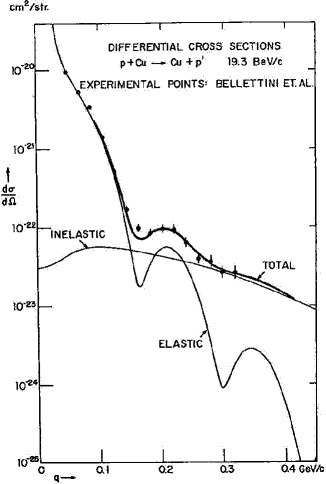
b:

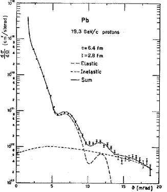
Figure 2: Elastic, inelastic and summed scattering calculated by Kofoed-Hansen for 19.3 GeV/$c$ protons incident on Cu (a) and by Matthiae for 19.3 GeV/$c$ protons incident on Pb (b). Experimental points from Bellettini et al [2].

I mention all of this because I want to tell you about another kind of application which is somewhat less elementary. Historically, however, it is a little bit older than the scattering measurements. When they began operating the 184” Berkeley cyclotron in 1947 they projected a beam of deuterons against a target of heavy nuclei. The first thing observed was, that when they sent in a beam of 180 MeV deuterons, they got out a forward travelling beam of 90 MeV neutrons. How did that happen? Well, Robert Serber gave a very simple explanation [3]. Here in Fig. 3a is the deuteron coming in, and as you see, it is just going to graze the edge of the nucleus. One must always assume that the intranuclear motions are slow, as indeed they are in the weakly bound deuteron. Now when the neutron and proton happen to be far apart,the proton is going to strike this opaque nucleus and be stripped away. What then will happen? Well, the neutron partner will be left alone and keep moving on. This is the process that Serber called stripping. (He actually named it after something that had been done in Los Alamos in a very different connection several years earlier.) There was something unknown at the time that Serber omitted from the calculation, and that is what has since become known as diffraction dissociation. Suppose the neutron and the proton happen at that moment of encounter to be closer together, as in Fig. 3b. Well, then nothing hits the nucleus, both the neutron and proton go forward, undeflected. But what is left, populated still by both the neutron and the proton, is a truncated version of the deuteron wave-function. Now the neutron-proton system has only one bound state, the deuteron ground state, so anything you do that chews away a part of the deuteron wave-function is going to leave a certain component of excited states present. As far as the excited state content of this funny wave-function is concerned, the neutron and proton will simply part company and separate. That describes the process of diffraction dissociation, and it was first noticed just 50 years ago [4], so we have now something of an anniversary. I should say that Good and Walker shortly after that, adopted this process as a kind of model for the behavior of the nucleons themselves at higher energies, and they gave it the name diffraction dissociation [5]. I too was thinking in those days about diffractive models for what neutrons and protons do when they produce small-angle sprays of particles in the forward direction. But if you are a theorist and try to say anything about this, you need a theory to back it up. Good and Walker were experimenters. They did not need any theory, they simply assumed that there is a process called diffraction dissociation, based on the analogy with the deuteron.

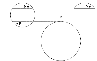
a: b:

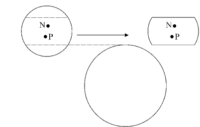
Figure 3: Illustration of a deuteron-nucleus collision. The deuteron is coming in from the left, grazing the edge of the nucleus. When the neutron and proton happen to be far apart (a), the proton strikes the nucleus and is stripped away. The neutron partner will be left alone and keep moving on. If the neutron and the proton are at the moment of encounter closer together (b), then nothing hits the nucleus, both the neutron and proton go forward, undeflected. A truncated version of the deuteron wave-function is left.

Now I’d like to persuade you that there are some things that go on in the diffraction theory that are not altogether obvious and have some relevance to work on heavy ion collisions. I am sorry to say, however, most of the things that are in this diffraction theory of nuclear collisions, are omitted from your heavy ion work, because you are ordinarily not very interested in small momentum transfer processes. Particle production processes, for example, typically involve large momentum transfers. So, after these omissions what is left is simply the geometrical substrate of diffraction theory, a kind of skeleton, and I find that my name is mentioned frequently in connection with an extremely nasty multiple integral that has to be done numerically. Well, this integral seems principally to take two different forms, I find in attending some of your lectures. One of these treats all collisions equally and simply sums up the total number of collisions that takes place. The other form was invented by some Polish friends of mine and I will talk about that in a moment.

Let us first talk about a single particle colliding inelastically with a nucleus having A constituents. We want to derive the cross section for all possible combinations of individual inelastic processes, whatever they may be:

$$\sigma_{\rm{part.prod.}}=\int\left\{1-(1-{\sigma_{\rm{in}}}t(b))^{A}\right\}d^{2}b\,.$$ (1)

Here ${\sigma_{\rm{in}}}$ is the relevant inelastic cross-section for nucleon-nucleon collisions. The function $t$ at the impact parameter $b$ is the effective thickness of a single nucleon and it is normalized to unity, $\int t(b)d^{2}b=1$. Now what is the probability $P_{n}$ that $n$ of these inelastic collisions take place? Well, you have to pick out a combination of $n$ nucleons from the $A$ of them. The number of ways you can do that is given by a familiar combinatorial coefficient, with the result that:

$$P_{n}={\left(\begin{array}[]{c}A\\ n\end{array}\right)}({\sigma_{\rm{in}}}t)^{n}(1-{\sigma_{\rm{in}}}t)^{A-n}\,.$$ (2)

Here you have the expression ${\sigma_{\rm{in}}}t$ raised to the $n$^th power, that is the probability for $n$ particular collisions to take place with $n$ nucleons. Then for the remaining $A-n$ nucleons such collisions must not happen. Eq. (2) simply counts all the ways these events can take place.

Now I want to generalize this model in a way that may interest you. I am going to assume that there is a number $\mu$ which is a kind of efficiency in a single collision for doing whatever process interests us. So let us say, the first collision, on a virgin nucleon produces one unit of whatever we are looking for. The second one only produces a fraction of that, a fraction we shall call $\mu$. The third one produces $\mu^{2}$, and so on. My Polish friends, when $\mu=0$, called this the wounded nucleon model [6]. I do not know what to call this more general model, but I think that by analogy with the way “pre-owned” cars are traded in America, this might be called the “used nucleon model.” If you ask what is the number of particles that get produced in these $n$ collisions, well, you have a finite geometrical series to sum, and here is the answer:

$$1+\mu+\dots+\mu^{n-1}=\frac{1-\mu^{n}}{1-\mu}\,.$$ (3)

Now let us put the pieces together. It is convenient to abbreviate the cross-section times the thickness function, by calling it $x={\sigma_{\rm{in}}}t(b)$. The average multiplicity of the event weights that finite geometrical sum with the probabilities we derived a moment ago. Now the steps that follow are just uninteresting algebra, but the result is very simple. What it does is to multiply the individual cross-sections by the number $1-\mu$, and then it renormalizes the entire expression by a factor of $1/\left(1-\mu\right)$.

Av. multiplicity $$= \Sigma_{n}P_{n}\frac{1-\mu^{n}}{1-\mu}$$ (4)

$$= \frac{1}{1-\mu}\Sigma{\left(\begin{array}[]{c}A\\ n\end{array}\right)}x^{n}(1-x)^{A-n}(1-\mu^{n})$$

$$= \frac{1}{1-\mu}\left\{(x+1-x)^{A}-(\mu x+1-x)^{A}\right\}$$

$$= \frac{1}{1-\mu}\left\{1-\left[1-(1-\mu)x\right]^{A}\right\}.$$

There are two limits for this expression. The one extreme, $\mu=0$, is pretty dramatic. It corresponds to a kind of automobile we once had in America called the Yugo. One collision and it is gone. In that case, the average multiplicity is just the same as the probability of at least one collision. And what you have there is the wounded nucleon model of my friends Bialas, Bleszinski, and Czyz [6]. On the other hand, if you take $\mu=1$ or, more correctly, let $\mu$ approach one as a limiting process, then the average multiplicity turns out to be $Ax$. It is just the average number of collisions in which you count all of them with equal weighting.

Now what does this mean when you have two nuclei colliding with one another? It yields a somewhat longer formula, but that is just the formula you have seen before for the wounded nucleon model except that it has some factors of $1-\mu$ inserted:

$$\langle\textrm{Mult}\rangle_{\mu} = \frac{A}{1-\mu}\int T_{A}(s)\left\{1-\left[1-(1-\mu){\sigma_{\rm{in}}}T_{B}(b-s)\right]^{B}\right\}d^{2}s$$ (8)

$$+ \frac{B}{1-\mu}\int T_{B}(s)\left\{1-\left[1-(1-\mu){\sigma_{\rm{in}}}T_{A}(b-s)\right]^{A}\right\}d^{2}s.$$

So the calculation is always very much the same as the one that has been done by each of the RHIC groups. However, there are the renormalizations by factors of $1-\mu$ involved, and in particular for $\mu=0$ the expression before us is just what has been called the number of participants, or in Poland the number of wounded nucleons. On the other hand when we let $\mu$ go to one, what it becomes is twice the total number of collisions. Not the number of collisions, but twice it, because every collision has two participants. It is the number of collided nucleons rather than the number of collisions. So this “used nucleon” model gives you a way of interpolating between the two limits that are discussed most, and it associates perhaps a new parameter $\mu$ with whatever sort of process interests you.

Now I want to change the subject altogether and begin to talk about quantum optics. For that, let me remind you of a famous sort of astronomical experiment first performed by two men trained as radio engineers, R. Hanbury Brown and R. Q. Twiss [7]. They used two radio antennas pointed at a radio source and chose to detect each signal separately to take away its high frequency component. They felt it would be much easier then to handle the remaining low frequency modulations that are present in such an astronomical signal. They sent those signals to a central point where they were multiplied together and averaged over time.

How does one analyze an experiment of that sort? It is very easy to show that there is an interference term present in the product of these two detected signals. That interference term is rather different from the interference terms one ordinarily encounters in 19^thcentury optics. Let us divide the field into two complex conjugate pieces, and talk then about the two complex fields that each oscillate with a single sign of the frequency:

$$E(r,t)=E^{(+)}(r,t)+E^{(-)}(r,t)\,\textrm{, and}$$ (9)

$$E^{(-)}(r,t)=\left\{E^{(+)}(r,t)\right\}^{*}\,.$$ (10)

Virtually all of traditional wave optics, that is essentially all of optics until the early 1950’s then can be discussed in terms of the lowest order field correlation function, which is an averaged product only quadratic in the field strengths:

$$G^{(1)}\equiv\langle E^{(-)}(r,t)E^{(+)}(r^{\prime},t^{\prime})\rangle\,.$$ (11)

But Hanbury Brown and Twiss were telling us that you have to deal with a quartic expression, because you have two detected signals each of which is quadratic in the field strengths:

$$G^{(2)}\equiv\langle E^{(-)}(r,t)E^{(-)}(r^{\prime},t^{\prime})E^{(+)}(r^{\prime},t^{\prime})E^{(+)}(r,t)\rangle\,.$$ (12)

That led them, I’m afraid, to a terrible dilemma. They were eager to perform the same interferometry with visible light as they had with the radiofrequency fields that they regarded as classical, but for a time fell victims to a great confusion about the quantum theory which has not entirely disappeared. To do the same sort of experiment with light quanta, they realized you obviously need to annihilate two quanta, one at each detector. When you read the first chapter of Dirac’s famous textbook in quantum mechanics [8], however, you are confronted with a very clear statement that rings in everyone’s memory. Dirac is talking about the intensity fringes in the Michelson interferometer, and he says,

Every photon then interferes only with itself. Interference between two different photons never occurs.

Now that simple statement, which has been treated as scripture, is absolute nonsense. First of all, the things that interfere are not the photons themselves, they are the probability amplitudes associated with different possible histories. You can obviously have different histories that involve more than one photon at a time. The intensity interferometry of Hanbury Brown and Twiss was indeed exploiting the interference of pairs of photons. But they were not completely persuaded, and I am not sure they were ever fully persuaded. Instead they chose to resolve the dilemma by doing another experiment that was both cleverer and more revolutionary than the experiments on determining the angular sizes of radiofrequency sources. Here, in Fig. 4 is their experimental setup [9]. Their light source is an extremely monochromatic discharge tube. The light from that goes to a half-silvered mirror, which sends beams to two separate photo-detectors. The random signals coming from those two detectors are multiplied together, as they were in their radiofrequency experiments and then averaged. What they found was a slight tendency for both of these photodetectors to go off together as they varied the position of one of them and thus the time delay between them. It was only a slight tendency toward correlation because in fact the effect was spread out over time by the rather poor resolution time of their detection equipment. The experiment was later repeated somewhat more accurately by Pound and Rebka [10]. Subsequent repetitions of this experiment have indicated that if you have very high resolving power in your counters, you can detect something approaching an increase of a factor of two in the coincidence rates for very short time delays.

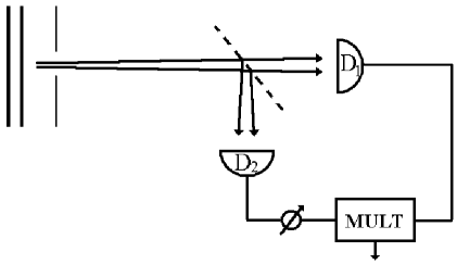
Figure 4: Setup of the Hanbury Brown – Twiss experiment. Light from an extremely monochromatic discharge tube goes to a half-silvered mirror, which sends beams to two separate photo-detectors. The random signals coming from those two detectors are multiplied together and then averaged.

Some nonsensical things were initially said about the interpretation of this experiment, but a correct interpretation was soon given by Purcell[11] on the basis of semi-classical reasoning and a classical formula for noise power he had quoted from the Radiation Laboratory Handbook. But there were other papers published that still misinterpreted the effect. One said that because of the very narrow linewidth and coherence characteristic of a laser beam, there should be a very dramatic Hanbury Brown – Twiss correlation in such a beam. I was very puzzled by that claim and published a brief note saying no, there will be absolutely no such effect at all in a laser beam, in fact no photon correlations whatever. But then that led back to the question, what is coherence? Optical coherence as it is usually construed deals only with the first or lowest order correlation function of Eq. (11), which is quadratic in the fields. You can define higher orders of coherence, in which the higher order correlation functions such as given by Eq. (12) will factorize. When they do factorize it wipes out the effect of photon bunching. The Hanbury Brown – Twiss correlation effect disappears completely. Well, all of the $G^{(n)}$’s can factorize, and in that case you can speak of full coherence. That holds in particular for what I have called the coherent states because they are eigenstates of the photon annihilation operators. When you annihilate a photon in those states the state doesn’t change. The annihilation operator just multiplies the state by a constant so that the correlation functions of all orders just factorize.

I had been able to show back in the early 50’s [13], that any classical or pre-determined current will radiate coherent states. That raises the question then, what is the effective current for a laser? The answer is, that in a laser there is a strongly oscillating transverse polarization current that radiates its beam. It is a very powerful current, but the electric charge does not go anywhere. It remains bound in the gas atoms. That in a nutshell is why a laser beam does not have a Hanbury Brown – Twiss correlation for its photons.

There is a fair-sized field that developed since then, which we now call quantum optics. In a sense it is really the study of time-dependent photon statistics. I would like to show you now in a minute or two that photon statistics can have something to say about heavy ion collisions. There is a very close parallel in some ways between the statistical analysis you do for emitted bosons, and the problems of quantum optics.

Let us suppose we are presented with a pure signal, which is represented by a coherent state $|\beta\rangle$. If you try counting the number of photons in that state for any length of time, you will always obtain a Poisson-distribution about the mean value $|\beta|^{2}$ :

$$p(n)=\frac{|\beta|^{2n}}{n!}\textrm{e}^{-|\beta|^{2}}\,.$$ (13)

Suppose, on the other hand, you are presented with a signal that consists of pure noise. That is to say you have a Gaussian distribution

$$P(\alpha)=\frac{1}{\pi\langle n\rangle}\textrm{e}^{-\frac{|\alpha|^{2}}{\langle n\rangle}}$$ (14)

of the amplitudes of coherent states. For that case you obtain a famous geometrical distribution for the number of photons that you count:

$$p(n)=\frac{1}{1+\langle n\rangle}\left(\frac{\langle n\rangle}{1+\langle n\rangle}\right)^{n}\,.$$ (15)

What happens when you superpose noise and signal? Well in the coherent state language it is very simple. You just displace the Gaussian distribution function by $\beta$. But when you do the calculation of the $n$-quantum probabilities, the distribution of the number of quanta you find is no longer so simple:

$$p(n)=\left(\frac{\langle n\rangle}{1+\langle n\rangle}\right)^{n}L_{n}\left(-\frac{|\beta|^{2}}{\langle n\rangle(1+\langle n\rangle)}\right)\textrm{e}^{-\frac{|\beta|^{2}}{1+\langle n\rangle}}\,.$$ (16)

There is nothing obvious about this result at all. The $L_{n}$ in it happens to be the $n$^th Laguerre-polynomial. Figure 5 shows you what that distribution looks like if the average number of quanta counted is 20. If the signal is purely coherent, you have the familiar Poisson distribution E. If it is pure noise on the other hand, you have the geometrical distribution, given by curve A. Curve B corresponds to half signal and half noise, and it still looks a great deal like the noise distribution. Curve D corresponds to corrupting the signal with only two quanta on the average. You have an average of 18 quanta from the coherent signal, and just two quanta of noise. A little noise goes a long way toward changing the distribution.

Let me now ask, can there be any coherence present in the heavy-ion output of pions, for example? Aren’t the violent collisions you study just about the most incoherent things you could possibly imagine? Well, let us consider the example of the simplest of all meson theories. We take the interaction to be that between a meson field $\phi(r,t)$ and a fixed source $\rho(r)$:

$$H_{\textrm{int}}=\int\rho(r)\phi(r,t)d^{3}r\,.$$ (17)

The ground state in that theory is in fact a coherent state, $\Pi_{k}|\alpha_{k}\rangle$. It happens to be a bound one; the pions can’t go anywhere. The amplitudes are as follows:

$$\alpha_{k}\propto\frac{\int\rho\textrm{e}^{-ikr}d^{3}r}{E(k)}\,,$$ (18)

where $E(k)$ is the energy for the $k$^th mode. Now if you were suddenly to wipe out this source density, that is to set it instantly equal to zero, what would happen? Of course you would have to supply energy to the field to do that. The coherent excitation would suddenly be set free, and you would have a coherent state of free pions, with no momentum correlation at all between them. Now suppose we don’t do anything so drastic as to wipe out the source $\rho$ but instead we replace $\rho$ suddenly by a wildly random source instead of a smooth source of any sort. That random source is going to produce random mode excitations, and the density operator that describes the field is going to be some sort of a distribution over a set of random amplitudes $\gamma_{k}$. The random excitations superposed upon the initially coherent state will lead to a density operator

$$\int P(\left\{\gamma_{k}\right\})\Pi_{k}|\alpha_{k}+\gamma_{k}\rangle\langle\alpha_{k}+\gamma_{k}|d^{2}\gamma_{k}.$$ (19)

Now the coherent excitation remains, and you can’t get rid of it. It remains there, but its contribution could be altogether swamped by the vast amount of noise an energetic collision adds to the field. The answer is nonetheless: Yes, you can indeed have some coherence present in this extremely incoherent output. It could be one of several reasons why the measured correlation functions for like pions do not rise to the value 2 for vanishing relative pion momenta.

Figure 5: Photon count distributions which would be measured in various superpositions of coherent (signal) and chaotic (noise) fields. Curve A represents the distribution for a pure noise field. The other curves represent the distribution for fields in which the noise and signal components would separately contribute the following average numbers: Curve B, 10 from noise and 10 from the signal; Curve C, 5 and 15; Curve D, 2 and 18; Curve E, 0 and 20, respectively.

References

-
[1]
R. J. Glauber, High Energy Collision Theory, in: Lectures in
Theoretical Physics, Vol I, ed. W. E. Brittin et al.
(Interscience
Publishers, New York, 1955), p. 315
R. J. Glauber, in: High Energy Physics and Nuclear Structure, ed. G. Alexander (North Holland Publishing Co., Amsterdam, 1967), p. 311;
R. J. Glauber, in: High Energy Physics and Nuclear Structure, ed. S. Devons (Plenum Press, New York, 1970), p. 207;
R. J. Glauber and G. Matthiae, Nucl. Phys. B 21, 135 (1970) - [2] G. Bellettini et al, Nucl. Phys. 79, 609 (1966)
- [3] R. Serber, Phys. Rev. 72, 1008 (1947)
- [4] R. J. Glauber, Phys. Rev. 99, 1515 (1955)
- [5] M. L. Good and W. D. Walker, Phys. Rev. 120, 1855 and 1857 (1960)
- [6] A. Bialas, M. Bleszynski and W. Czyz, Nucl. Phys. B 111, 461 (1976)
- [7] R. Hanbury Brown and R. Q. Twiss, Phil. Mag. 45, 663 (1954)
- [8] P. A. M. Dirac, The Principles of Quantum Mechanics. Third edition (Oxford University Press, Oxford, 1947), p. 9
- [9] R. Hanbury Brown and R. Q. Twiss, Nature 177, 27 (1956), Proc. Roy. Soc. (London) A242, 300 (1951), Proc. Roy. Soc. (London) A243, 291 (1957)
- [10] G. A. Rebka and R. V. Pound, Nature 180, 1035 (1957)
- [11] E. M. Purcell, Nature 178, 1449 (1956)
-
[12]
R. J. Glauber, Phys. Rev. Lett 10, 84 (1963);
R. J. Glauber, Phys. Rev. 130, 2529 (1963);
R. J. Glauber, Phys. Rev. 131, 2766 (1963);
R. J. Glauber, in: Quantum Optics and Electronics, ed. C. de Witt et al (Gordon and Breach, Inc., New York, 1965), p. 63 - [13] R. J. Glauber, Phys. Rev. 84, 395 (1951)