Beyond mean-field study of excited states: Analysis within the Lipkin model

Abstract

Beyond mean-field methods based on restoration of symmetries and configuration mixing by the generator coordinate method (GCM) enable to calculate on the same footing correlations in the ground state and the properties of excited states. Excitation energies are often largely overestimated, especially in nuclei close to magicity, even when transition probabilities are well-described. We analyse here the origin of this failure. The first part of the paper compares realistic projected GCM and QRPA calculations for selected Sn isotopes performed with the same effective Skyrme interaction. Although it is difficult to perform RPA and GCM calculations under exactly the same conditions, this comparison shows that the projected GCM overestimates the RPA results. In the second part of this paper, we compare GCM and RPA in the framework of the exactly solvable Lipkin-Meshkov-Glick model. We show that the discretized GCM works quite well and permits to obtain nearly exact results with a small number of discretization points. This analysis indicates also that to break more symmetries of the nuclear Hamiltonian in the construction of the GCM basis is probably the best way to improve the description of excited states by the GCM.

I Introduction

Self-consistent mean-field methods are one of the standard microscopic approaches in nuclear structure theory RMP . At present, they are the only available microscopic method that can be systematically applied on a large scale for medium and heavy nuclei. The full model space of occupied states can be used, which removes any distinction between core and valence particles and the need for effective charges. This allows the use of a universal effective interaction, universal in the sense that it can be applied for all nuclei throughout the periodic chart.

Despite its successes, the self-consistent mean-field method has a number of well-known limitations. From a conceptual point of view, the mean-field approach is designed to describe mainly ground-state properties, and gives very limited access to excited states. This is in contrast to the microscopic methods that are available for light nuclei, like the no-core shell model and the shell-model Monte-Carlo, which also describe excitation spectra. A systematic way to resolve these problems is offered by symmetry restoration and configuration mixing. Several groups now develop methods going beyond a mean-field approach based on the generator coordinate method (GCM), either with non-relativistic Skyrme Val00a ; BH03 or Gogny Rod00a interactions, or with relativistic Lagrangians Nik06a , see also Egi04a ; enam and references given therein. The aim is to obtain a global description of ground states, including collective correlations which cannot be included in a mean-field approach, even at the effective interaction level, and of excited states of all nuclei in a single, unified method.

An introduction to the method that we develop along these lines can be found in Ref. enam . First applications have demonstrated that such a method permits to describe the energies of low-lying collective excitations and electric transition probabilities, in-band and out-of-bands. However, in many cases it has also been found that whenever states can be grouped into rotational bands, the spectra obtained with the GCM are too spread and that the excitation energies are too high. For spherical nuclei, in particular those close to doubly-magic ones, the low-energy collective spectra are only qualitatively in agreement with the data. This feature is well illustrated by a detailed study of the quadrupole and octupole modes of nuclei around ²⁰⁸Pb in Ref. Hee01 : the excitation energies of the first $3^{-}$ and $2^{+}$ states are overestimated by more than 1 MeV. On the other hand, the energies of giant resonances were found to be more realistic, as was also shown in Ref. SH96 .

The origin of this problem is not obvious and it cannot be expected to be unique. A possible source of error could be the inadequacies of effective interactions to describe spectra. It is certainly an appealing feature of the projected GCM that the same effective interaction can be used to generate the mean-field states and to perform their mixing. However, existing interactions are still far from describing all nuclei with a similar high quality Gor02a ; Ber05a ; Ben06a . Furthermore, they have been adjusted exclusively at the level of the mean-field approximation and on ground state properties, with at most constraints on the values of global parameters, like the effective masses or the compressibility, deduced from the systematics of excited states. There is no guarantee that such effective interactions will correctly predict spectra, although, up to now, GCM results are encouraging, and, in most cases, in good qualitative agreement with available data. Another source of uncertainty of the GCM comes from the choice of the variational space in which the configuration mixing is performed. It is usually constructed by introducing constraints on one or a few collective variables related to the shape of the nuclear density in the mean-field equations. Such a choice may be more appropriate to describe the properties of ground states than those of excited states, for which additional degrees of freedom might have to be included.

Up to now, these problems have not been addressed in a systematic way, with the exception of the detailed study of ²⁰⁸Pb and its isotopes mentioned above but which did not include the restoration of rotational symmetry. Rather than to repeat the same kind of analysis as in Ref. Hee01 , we will adopt here another strategy. We will first compare results obtained with the same effective interaction using either the GCM or the random phase approximation (RPA). The RPA is an alternative microscopic method to calculate collective excitations, relying also on the existence of a nuclear mean field. The RPA is very well adapted to the description of collective excitations in spherical nuclei. This will enable us to separate the problems related to the effective interactions from those related to the method. We will make this comparison for two Sn isotopes, the doubly magic ¹³²Sn and ¹²⁰Sn, performing the GCM and RPA calculations under conditions as close as possible. We will see that the results differ in a manner that raises questions about the degrees of freedom that are explicitly included in the GCM. However, significant differences between both methods cannot be easily eliminated and the comparison between both models cannot be fully conclusive.

One therefore needs a view on the problem from another perspective. Exactly solvable models constitute a very fruitful ground for the test of and comparison between many-body methods. They also permit to explore new developments at a very limited cost. For this purpose, we need a model where collective variables similar to deformations can be introduced and where a discretized version of the GCM can be defined in a way similar to that of the realistic applications. The Lipkin-Meshkov-Glick (LMG) model, introduced in Ref. LMG65 , has the required properties. Depending upon the strength of the interaction, two different kinds of solutions are obtained at the Hartree-Fock (HF) level RingSchuck : ”spherical” ones at low values of the strength, and ”deformed” ones beyond a critical strength. The second part of the paper is devoted to a detailed discussion of the LMG model.

II Comparison between the QRPA and projected GCM on Sn isotopes

II.1 Technical aspects

Our beyond mean-field method has already been presented in details and applied to a large number of nuclei Val00a ; BH03 ; BFH03 ; DBBH03 ; BHB04 ; BBH05 ; BBH06 . Let us here summarize those of its features which are essential for a critical comparison with the RPA.

The starting point of the method is a set of constrained mean-field calculations, with the axial quadrupole moment as a constraining operator. The wave functions obtained for a discrete set of quadrupole moments are projected on good particle numbers and on angular momentum. For each value of the angular momentum, the projected wave functions are mixed with respect to the quadrupole moment by the generator coordinate method (GCM), leading for each angular momentum to a collective wave function spread over a range of deformations.

The same effective interactions, the Skyrme SLy4 sly4 in the mean-field (particle-hole) channel and a density-dependent zero-range force pairing in the pairing (particle-particle) channel with a strength of $-1250$ MeV fm³ are used for the construction of the mean-field wave functions and for the calculation of the GCM matrix elements. The BCS subspace is limited to an energy range of 5 MeV above and below the Fermi level.

Pairing correlations are a necessary ingredient of a GCM calculation: the Hartree-Fock Slater determinants corresponding to two deformations, for which the number of occupied single-particle states of a given symmetry is different, are orthogonal. This feature makes a GCM calculation numerically unstable. The problem is cured by the partial occupation of single-particle levels due to pairing. As BCS pairing correlations collapse whenever the density of single-particle levels around the Fermi surface is low, we use the Lipkin-Nogami (LN) method to ensure that pairing correlations are present for all values of the quadrupole moment.

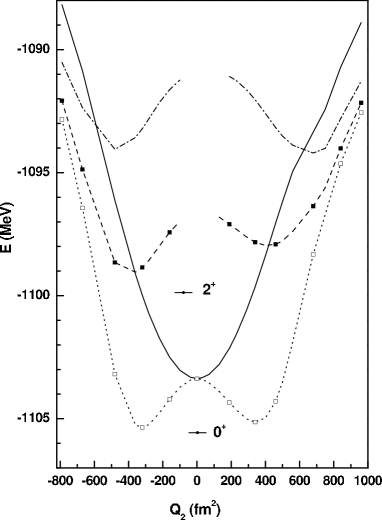
Figure 1: Projected energy curves as a function of the quadrupole moment for ¹³²Sn. The particle-number projected mean-field deformation energy is represented by a solid line, while dotted, dashed and dash-dotted lines correspond to projected mean-field energies for $J=0$, 2, and 4, respectively.

II.2 Results for Sn isotopes

Let us first compare GCM and RPA predictions for the first excited $2^{+}$ state in a doubly magic nucleus, ¹³²Sn, which has already been extensively studied by the RPA TENS02 ; colo03 ; giam03 .

In Fig. 1, the mean-field energy curve is shown together with the $J=0$ to 4 projected energy curves as a function of the quadrupole moment. As usual, the projected states are labelled by the deformation of the mean-field state which is projected. The topography of the projected curves is typical for nuclei which have a well defined spherical mean-field ground state BBH06 . After projection, there are two nearly degenerate $J=0$ minima corresponding to two slightly deformed mean-field configurations, oblate and prolate. The energy gain is moderate, of the order of 2 MeV, with a marginal extra gain of 210 keV due to configuration mixing. The collective GCM wave functions are plotted in Fig. 2 for $J=0$ and 2.

In Table 1, we compare the energies and $B(E2)$ values obtained in projected GCM and RPA calculations based on the same effective interaction colo03 ; colo04 with the experimental data ram01 ; rad05 . The excitation energy of the $2^{+}$ state is overestimated by both methods. Within the RPA framework, one can show that, for Sn isotopes, the inclusion of phonon couplings decreases the excitation energy of the $2^{+}$ state and reduces the $B(E2)$ transition probability, although this decrease is less pronounced in ¹³²Sn than in lighter isotopes SVG04 . Note also that the energy centroid of the isoscalar giant quadrupole resonance is predicted correctly by the GCM at 12.45 MeV, close to the value given by the empirical systematics $63$ $A^{-1/3}$ MeV.

We have performed a similar calculation for ¹²⁰Sn for which neutron pairing correlations are present in the ground state and for all deformations. Results are compared in Table 2 with a RPA calculation colo04 and with experiment ram01 . Again, we find a discrepancy between the RPA and GCM predictions for the excitation energy of the low-lying $2^{+}$ state, whose energy is significantly larger in the GCM calculation than in RPA. The $B(E2)$ value obtained within GCM is closer to the experimental value than the RPA value. This result is consistent with our findings for other systems that transition moments are in most cases much better described than excitation energies, and suggests that also for nuclei that are spherical at the mean-field level the geometrical properties of excited states are better described by the GCM than their excitation energies. This may be related to the fact that the components of the $2^{+}$ states corresponding to two-quasi-particle excitations breaking time reversal invariance are completely missing from the GCM model space and that these components have a larger contribution to energies than to transition probabilities.

Table 1: Excitaion energy (in MeV) and $B(E2)$ value (in e² fm⁴) for up transition to the first $2^{+}$ state in ¹³²Sn.

Method	Energy (MeV)	B(E2$\uparrow$)
GCM	5.69	630
Particle-hole RPA	5.13	1370
Experiment	4.04	1100$\pm$300

Table 2: Excitation energy (in MeV) and $B(E2)$ value (in e² fm⁴) for up transition to the first $2^{+}$ state in ¹²⁰Sn

Method	Energy (MeV)	B(E2$\uparrow$)
GCM	2.40	1350
Quasiparticle RPA	1.44	440
Experiment	1.17	2020$\pm$40

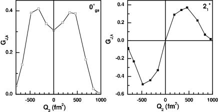
Figure 2: Collective GCM wave functions for the ground state and the first $2^{+}$ state of ¹³²Sn.

Since neither RPA nor GCM do satisfactorily reproduce the experimental energies and transition probabilities for both Sn isotopes, it is tempting to conclude that the Skyrme effective interaction is not fully adequate to describe low energy excitations in this mass region.

Besides this problem of interaction, a direct comparison between RPA and GCM results shows a discrepancy and a suspicion that the GCM variational subspace as defined in actual applications is not as rich as the RPA one, in particular, at small deformations, where two-quasi-particle excitations breaking time-reversal invariance are not included in our GCM. Unfortunately, there are several differences between both calculations, which might affect their comparison, some of them being hard to eliminate.

In both cases, the same effective interaction is used in the mean-field channel. However, since ¹³²Sn is a doubly-magic nucleus, there are no pairing correlations in the spherical ground state with either a BCS or a Bogoliubov treatment of pairing. Therefore, there is no pairing at all in an RPA approach, in contrast to the GCM. As soon as the quadrupole deformation of the constrained mean-field state is sufficiently large (in this case, 500 fm²), pairing correlations are present also in the BCS method. As already mentioned above, the GCM requires generating wave functions which vary smoothly along the collective path, which is enforced using of the LN prescription; hence, in our GCM pairing correlations are present in all states, even in the spherical mean-field configuration of ¹³²Sn.

Another difference between the RPA calculation of colo04 and our GCM calculation is that the Coulomb and the spin-orbit residual interactions are not included in the RPA, but are always present in the GCM. The effect of these terms has been very recently studied by Terasaki et al. ter05 and Péru et al. Per05a . The inclusion of the Coulomb residual interaction raises the $2^{+}$ excitation energy by 200 to 300 keV.

Some recent studies have also pointed out that the RPA has shortcomings which are usually forgotten. As shown by Johnson and Stetcu, the QRPA does not restore symmetries exactly Ste03a . Moreover, in some cases, the RPA predicts poorly the ground state correlation energies Ste02a , the excitation energies Joh02a and $B(E2)$ values Ste03a .

Still, it seems clear that the GCM overestimates excitation energies in spherical nuclei close to magicity. On the other hand, since it looks difficult to remove all the differences between GCM and RPA calculations, the use of a model that can be exactly solved seems to be the most appropriate way to deepen the present analysis.

III Excited states in the Lipkin-Meshkov-Glick model

III.1 The model

Lipkin, Meshkov, and Glick introduced an exactly solvable model LMG65 , usually called ”Lipkin model” or ”LMG model” in the literature, that has been widely used to test methods of approximation for the nuclear many-body problem.

The model consists of $N$ fermions distributed in two $N$-fold degenerate shells separated by an energy $\varepsilon$. In their original paper, two different Hamiltonians were proposed. The one which is the most usually studied contains a monopole-monopole interaction and is given by:

$$\hat{H}=\varepsilon J_{0}-\frac{1}{2}V(\hat{J}_{+}\hat{J}_{+}+\hat{J}_{-}\hat{J}_{-}),$$ (1)

where $V$ is the interaction strength and $\hat{J}_{0}$, $\hat{J}_{\pm}$ are quasi-spin operators LMG65 ; ho73 ; RingSchuck

$$\hat{J}_{0} = \frac{1}{2}\sum_{p=1}^{N}(\hat{c}_{+p}^{\dagger}\hat{c}_{+p}-\hat{c}_{-p}^{\dagger}\hat{c}_{-p}),$$

$$\hat{J}_{+} = \sum_{p=1}^{N}\hat{c}_{+p}^{\dagger}\hat{c}_{-p},$$

$$\hat{J}_{-} = \hat{J}_{+}^{\dagger}.$$ (2)

with the algebra

$$[\hat{J}_{+},\hat{J}_{-}]=2\hat{J}_{0},\qquad[\hat{J}_{0},\hat{J}_{\pm}]=\pm\hat{J}_{\pm}.$$ (3)

The operators $\hat{c}_{+p}^{\dagger}$ and $\hat{c}_{-p}^{\dagger}$ create a particle in the upper or lower shells, respectively, where $p$ labels the $N$ degenerate levels within the shells. The operator $\hat{J}_{0}$ measures half of the difference between the number of particles in the upper and the lower levels.

The exact wave functions are eigenstates of two operators, the total quasispin operator $\hat{J}^{2}=\frac{1}{2}(\hat{J}_{+}\hat{J}_{-}+\hat{J}_{-}\hat{J}_{+})+\hat{J}_{0}^{2}$ with eigenvalue $J(J+1)$, and a signature operator $e^{i\pi\hat{J}_{0}}$, which, for an even number of particles, has two eigenvalues equal to $\pm 1$. Therefore, as discussed in detail in Ref. LMG65 , the interaction does not mix states which have different eigenvalues of $\hat{J}^{2}$ and $e^{i\pi\hat{J}_{0}}$ and the Hamiltonian matrix splits into blocks, which are multiplets in $J$ of order $2J+1$. The multiplets separate further into blocks of size of $J$ and $J+1$ corresponding to the two values for the signature.

To understand the connection between the LMG model and realistic nuclear models, it is interesting to identify the structure of its eigenstates WN . In the limit of vanishing interaction strength $V=0$, the exact ground state corresponds to an independent particle state with all the lower single-particle levels occupied, while the exact first excited state is given by a 1p-1h excitation on top of the ground state, the second excited state by 2p-2h excitations, etc.

As the Hamiltonian does not mix states which different $J$ values, the exact wave functions are linear combinations of the $2J+1$ eigenfunctions of the operator $\hat{J}_{0}$ within a multiplet of given $J$ LMG65 . There is one state of each possible $n$p-$n$h content in each multiplet. The non-interacting ground state has $J_{0}=-N/2$, and belongs to the multiplet with maximum $J$, i.e. $J=N/2$. The first non-interacting excited state is a 1p-1h state which has $J_{0}=-N/2+1$. Pure 1p-1h states are admixtures of states from the $J=N/2$ and $J=N/2-1$ multiplets, while pure 2p-2h states are admixtures of states within the $J=N/2$, $J=N/2-1$ and $J=N/2-2$ multiplets, etc for higher $n$p-$n$h excitations until $n=N$.

For small values of the interaction strength $V$, the mixing within the multiplets should be small and low-lying levels should have a similar structure as the non-interacting ones. By contrast, for large values of $V$, the eigenstates will exhibit a complicate mixing of many p-h excitations. Thus, the model exhibits a transition between shell-model-like states and collective states.

III.2 Mean-Field Approximation

In mean-field, or Hartree-Fock (HF), approximation, the many-body wave function $|\alpha,\varphi\rangle$ is given by a Slater determinant

$$|\alpha,\varphi\rangle=\prod_{p=1}^{N}\hat{a}_{0p}^{\dagger}|-\rangle,$$ (4)

characterized by two real degrees of freedom $\alpha$ and $\varphi$, that will be specified below. The particle- and hole-creation operators of the corresponding HF single particle basis are given by a unitary transformation among the operators corresponding to the non-interacting basis RingSchuck ; ho73 :

$$\left(\begin{array}[]{c}\hat{a}_{1p}^{\dagger}\\ \hat{a}_{0p}^{\dagger}\end{array}\right)=\left(\begin{array}[]{cc}\cos(\alpha)&-\sin(\alpha)\,e^{-i\varphi}\\ \sin(\alpha)\,e^{i\varphi}&\cos(\alpha)\end{array}\right)\left(\begin{array}[]{l}\hat{c}_{+p}^{\dagger}\\ \hat{c}_{-p}^{\dagger}\end{array}\right).$$ (5)

The subscripts 0 and 1 denote hole and particle states, respectively. The variables $\alpha$ and $\varphi$ vary both in the interval $[-\pi/2,\pi/2]$. They can be identified as constraints, that, due to the low dimensionality of the LMG model, map the entire space of mean-field states. New quasi-spin operators corresponding to the states with finite $\alpha$ and $\varphi$ can be easily constructed, as described, for example, in ho73 . An alternative manner to write the constrained HF states will be useful in the context of the GCM. Using the Thouless theorem T60 , the normalized constrained HF states $|\alpha,\varphi\rangle$ can be obtained from the non-interacting ground state, that corresponds to $\alpha=\varphi=0$, as

$$|\alpha,\varphi\rangle=\cos^{N}(\alpha)\exp\left[\tan(\alpha)\exp(i\varphi)\hat{J}_{+}\right]|\alpha=0,\varphi=0\rangle.$$ (6)

A pointed out by Bhaumik et al. Bha81a , the constrained HF states of the LMG model can also be formulated in the language of coherent states, which allows to make use of generating functional techniques to calculate matrix elements Zha90a .

The constrained HF ground-state energy is a function of the variables $\alpha$ and $\varphi$:

$$E_{gs}^{\text{HF}}(\alpha,\varphi)=-\frac{\varepsilon N}{2}\left[\cos(2\alpha)+\frac{1}{2}\chi\sin^{2}(2\alpha)\cos(2\varphi)\right],$$ (7)

where

$$\chi=\frac{\left(N-1\right)V}{\varepsilon}.$$ (8)

Note that, for a given value of $\alpha$, the lowest HF state always corresponds to $\varphi=0$. The eigenvalues of the single-particle Hamiltonian, usually called single-particle energies, depend on $\alpha$ only for any mean-field state $|\alpha,\varphi\rangle$.

One can identify the variable $\alpha$ as a deformation parameter. There is a phase transition at $\chi=1$ from a spherical ($\alpha=\varphi=0$) to a ”deformed” ground state. In the latter case, the value of $\alpha$ is obtained by solving the equation $\chi\cos(2\alpha)=1$. The phase transition and the properties of exact and approximated ground states in this regime were first discussed by Agassi et al. Aga66a .

While the HF states remain eigenstates of $\hat{J}^{2}$, ”deformed” HF states break the signature symmetry of the exact solutions (which is often called ”parity” in the literature) for any non-zero value of $\alpha$. The HF states mix the $n$p-$n$h states with even and odd $n$ within a given $J$ multiplet. As a consequence, the constrained HF states for non-zero interaction strength contain 0p-0h, 1p-1h, 2p-2h, 3p-3h etc states. The $n$p-$n$h components with even and odd $n$ can be separated with a projection operator Aga66a ; Rob92a . Due to the simple structure of the LMG model with one relevant coordinate only, minimization of the energy obtained by projection after variation is equivalent to projection before variation Rob92a .

The signature symmetry is a discrete symmetry, in contrast to the continuous rotational symmetry broken in nuclei with a quadrupole deformation. Li et al. Li70a have introduced a generalization of the LMG model that can been used to test techniques for approximate angular-momentum projection, see Hag00a and references therein. The structure of the original LMG model is closer to parity projection in octupole-deformed nuclei Rob92a .

The interpretation of the $\varphi$ degree of freedom is less intuitive. It enters the HF states as a phase. It is explored by time-dependent HF (TDHF) states, hence a necessary ingredient of any dynamical model KLDG80 ; Kri77a . Using the variables $\alpha$ and $\varphi$, one can form a set of two canonically conjugate variables with which, for example, the time-dependent HF equations can be transformed to classical equations of motion KLDG80 .

III.3 Random phase approximation

The RPA of the LMG model was formulated for the first time in Ref. LMG65 . The RPA is usually constructed on top of the ”spherical” HF state $|\alpha=0,\varphi=0\rangle$, which is the ground state for $\chi<1$. In this regime, the RPA phonon creation operator, defined as a superposition of all possible 1p-1h excitations, is given by

$$\hat{Q}^{\dagger}=\frac{1}{\sqrt{N}}(X\hat{J}_{+}-Y\hat{J}_{-}).$$ (9)

One assumes that the ground state is the RPA phonon vacuum $|0\rangle$, i.e. $\hat{Q}|0\rangle=0$. The first excited state is given by $\hat{Q}^{\dagger}|0\rangle$ with the normalization condition:

$$\langle 0|[\hat{Q},\hat{Q}^{\dagger}]|0\rangle=X^{2}-Y^{2}=1.$$ (10)

Profiting from the simplicity of the LMG model, the authors of LMG65 have solved $\hat{Q}|0\rangle=0$ exactly. The usual way is to solve the RPA equations in the space of 1p-1h excitations by linearization. Making use of the equation-of-motion approach Row68a ; R70 :

$$\langle 0|[\delta\hat{Q},[\hat{H},\hat{Q}^{\dagger}]]|0\rangle=(E-E_{0})\langle 0|[\delta\hat{Q},\hat{Q}^{\dagger}]|0\rangle,$$ (11)

where $E$ is the absoute energy of the RPA state, and $E_{0}$ the energy of the RPA ground state, one obtains the RPA equations:

$$\left(\begin{array}[]{cc}\mathcal{A}&\mathcal{B}\\ -\mathcal{B}&-\mathcal{A}\end{array}\right)\left(\begin{array}[]{c}X\\ Y\end{array}\right)=(E-E_{0})\,\left(\begin{array}[]{c}X\\ Y\end{array}\right),$$ (12)

where $\mathcal{A}=\varepsilon$ and $\mathcal{B}=-(N-1)\,V=-\varepsilon\chi$.

From these equations, the excitation energy of the first excited state of the Hamiltonian (1) within the RPA is found to be

$$E-E_{0}=\varepsilon\sqrt{1-\chi^{2}}.$$ (13)

This energy is equal to zero for $\chi=1$, where the system undergoes a phase transition, and becomes imaginary for even larger values of $\chi$.

The RPA is explicitly constructed as a superposition of 1p-1h states; hence, it automatically contains the right physics of the lowest excited state in the limit $\chi\to 0$ and should be accurate in the limit of small $\chi$.

The RPA correlation energy RingSchuck in the ground state is given by:

$$E_{gs}=-\frac{\varepsilon N}{2}+\frac{1}{2}(\omega-\varepsilon).$$ (14)

III.4 Generator coordinate method

III.4.1 Continous GCM

Most applications of the GCM to the LMG model are restricted to a study of the GCM ground state and test the correlations in the ground-state Par68a . In such cases, one can take the “deformation” $\alpha$ as a single generator coordinate. We are here also interested in the description of excited states and will also introduce $\varphi$ as a generator coordinate.

One can write the $N$-particle GCM wave functions as a linear combination of the constrained HF states $|\alpha,\varphi\rangle$ (6) with an unknown weight function $f_{k}\left(\alpha,\varphi\right)$

$$|\Psi_{k}\rangle=\int_{-\frac{\pi}{2}}^{\frac{\pi}{2}}d\alpha\int_{-\frac{\pi}{2}}^{\frac{\pi}{2}}d\varphi\;f_{k}(\alpha,\varphi)\;|\alpha,\varphi\rangle.$$ (15)

Variation of the energy yields the so-called Hill-Wheeler-Griffin (HWG) equation Hil53a , an integral equation for $f_{k}(\alpha,\varphi)$

$$\int_{-\frac{\pi}{2}}^{\frac{\pi}{2}}d\alpha\int_{-\frac{\pi}{2}}^{\frac{\pi}{2}}d\varphi\;\left(\langle\alpha^{\prime},\varphi^{\prime}|\hat{H}|\alpha,\varphi\rangle-E_{k}\langle\alpha^{\prime},\varphi^{\prime}|\alpha,\varphi\rangle\right)\,f_{k}\left(\alpha,\varphi\right)=0.$$ (16)

The two kernels entering Eq. (16) are the norm kernel

$$\langle\alpha^{\prime},\varphi^{\prime}|\alpha,\varphi\rangle=\left[\cos(\alpha)\cos(\alpha^{\prime})+\sin(\alpha)\sin(\alpha^{\prime})e^{i(\varphi-\varphi^{\prime})}\right]^{N},$$ (17)

and the Hamiltonian kernel

$$\langle\alpha^{\prime},\varphi^{\prime}|\hat{H}|\alpha,\varphi\rangle = -\frac{\varepsilon N}{2}\langle\alpha^{\prime},\varphi^{\prime}|\alpha,\varphi\rangle$$

$$\times\frac{\cos^{2}(\alpha)\cos^{2}(\alpha^{\prime})-\sin^{2}(\alpha)\sin^{2}(\alpha^{\prime})e^{2i(\varphi-\varphi^{\prime})}+\chi\left[\sin^{2}(\alpha)\cos^{2}(\alpha^{\prime})e^{2i\varphi}+\cos^{2}(\alpha)\sin^{2}(\alpha^{\prime})e^{-2i\varphi^{\prime}}\right]}{\left[\cos(\alpha)\cos(\alpha^{\prime})+\sin(\alpha)\sin(\alpha^{\prime})\;e^{i(\varphi-\varphi^{\prime})}\right]^{2}}.$$

A set of orthonormal collective wave functions are obtained by an integral transformation of $f_{k}$

$$G_{k}(\alpha^{\prime},\varphi^{\prime})=\int_{-\frac{\pi}{2}}^{\frac{\pi}{2}}d\alpha\int_{-\frac{\pi}{2}}^{\frac{\pi}{2}}d\varphi\,\langle\alpha^{\prime},\varphi^{\prime}|\alpha,\varphi\rangle^{\frac{1}{2}}f_{k}(\alpha,\varphi).$$ (18)

The HWG integral equation can be solved exactly RingSchuck . Thanks to the simplicity of the LMG model, the GCM with a single generator coordinate $\alpha$ gives already the exact solutions of the model. The GCM is build on signature-symmetry breaking constrained HF states; hence, a priori the GCM wave function mixes 0p-0h, 1p-1h, 2p-2h, 3p-3h etc states. However, one can easily see that the signature symmetry is restored by mixing of HF wave functions corresponding to $\pm\alpha$ with weights equal in modulus, which comes out automatically from Eqn. (15). This situation is similar to realistic applications of the GCM when a discrete symmetry, like parity, is broken at the mean-field level but not for continuous symmetries like rotations.

III.4.2 Discretized GCM

In realistic calculations Val00a ; BH03 ; Rod00a ; Nik06a , the HWG equation is solved by discretization of the collective variables

$$|\Psi_{k}\rangle=\sum_{\alpha}\sum_{\varphi}f_{k}(\alpha,\varphi)\;|\alpha,\varphi\rangle.$$ (19)

The discretized GCM equations are obtained by replacing all integrals in Eqns. (15-18) by sums over discretization points. The integral equation (16) becomes a matrix equation which can be solved by diagonalization.

As our aim is to understand why the GCM overestimates excitation energies in realistic applications, we will solve the HWG equation of the LMG model by discretization. Since the continuous GCM permits to find the exact eigenstates of the LMG Hamiltonian, the number of discretization points must be small enough to avoid a trivial reproduction of the exact solution.

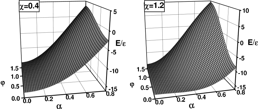
Figure 3: Mean-field potentials for two values of the interaction strength, $\chi=0.4$ and $\chi=1.2$, for $N=30$ particles.

We have solved the LMG model for 30 and 50 particles, with a discretization on meshes symmetric around $0$ in $\alpha$ and $\varphi$ and with an odd number of points. The meshes in $\alpha$ and $\varphi$ have been limited to the region in which the collective wave function has a sizable amplitude, typically less than half the total range of variation of $\alpha$. The mean-field potentials that are obtained for two values of $\chi$, above and below the phase transition, are plotted in Fig. 3. The mean-field ground state corresponds to $\alpha$ and $\varphi$ equal to zero when $\chi$ is smaller than 1, and to a non-zero value of $\alpha$ otherwise. The energy surface is very flat for small values of $\varphi$; it is only when $\alpha$ is large that the energy increases rapidly with $\varphi$. Such a topography is representative of the deformation energy curve that is obtained for spherical nuclei ($\chi<1$) and for nuclei soft as a function of deformation ($\chi>1$).

Figure 4: Comparison between the exact and GCM energies of the first three states of the LMG model for 30 particles. The solid lines are the exact result, while the dashed and dotted lines represent the GCM solutions obtained with the two different meshes (see text) with seven points in $\alpha$. The HF results are indicated by a dash-dotted line.

In Fig. 4, the exact and GCM energies for the ground state and for the first two excited states are plotted as a function of the two-body interaction strength $\chi$ for a system of 30 particles. We have used $\alpha$ as the only generator coordinate. The GCM equations are solved with 7 equidistant discretization points chosen in the region where the collective wave functions have a sizeable amplitude. In realistic applications of the GCM, the overlap kernel is used to define the mesh, the requirement being that the overlap between two adjacent points is of the order of 0.8. However, in the LMG model, this kernel does not depend on the two-body interaction strength. Since we want to be as close as possible to realistic applications, where the exact solutions are not known, we have taken the same mesh for all interaction strengths. From the collective wave function obtained for a value of $\chi$ around 0.5, we have chosen points in the interval ($-0.707$, $+0.707$). Since the wave functions of the model are either even or odd with respect to $\alpha$, only four discretization points are significant.

For $\chi<1$, the HF ground-state energy does not depend on $\chi$, as the ground state is always ”spherical”. The correlations beyond mean-field significantly improve the HF result for the ground state and bring it very close to the exact value for all values of the interaction strength. The situation is less satisfactory for excited states: in particular, their excitation energies are far from the exact values when the interaction is switched off, while the HF method gives the exact energies. The discretized GCM becomes more accurate than HF only for $\chi$ larger than 0.25 for the second excited state and than 0.45 for the first one.

To understand this surprising result, let us analyse in more details how the continuous GCM works in the $\chi=0$ limit. Let us first note that, while the exact ground state wave function, corresponding to $\alpha$ and $\varphi$ equal to zero, is included in the generating functions $|\alpha,\varphi\rangle$, the first excited states corresponding to pure 1p-1h and 2p-2h excitations are not. One can easily verify that the weight functions that permit to extract the exact eigenstates are the Dirac $\delta(\alpha)$ distribution for the ground state, its first derivative for the first excited state and combination of $\delta(\alpha)$ and its derivatives for higher excitations. The collective wave functions, given by equation (18), are regular functions but with rather sharp peaks. One of them is located at $\alpha$ equal to 0 for even signature states, while the odd signature states vanish at 0. Moreover, for very small values of $\chi$, the collective wave-functions have very small amplitudes at the most extreme mesh points, leaving only a very small number of significant discretization points.

Replacing one of the mesh points by a point close to the extrema of the wave functions of the first and second excited state for $\chi$ equal to zero, the discretized GCM results become very close to the exact values for the three first states and for low interaction strengths. For the first excited state, which has a node at the origin, this discretization is superior to the one based on the $\chi=0.5$ ground state wave function up to $\chi=0.75$.

Figure 5: Comparison between the exact and GCM energies of the first three states of the LMG model for a system with $N=50$. Two generator coordinates, $\alpha$ and $\varphi$ are used in the GCM. The exact result are represented by solid lines. The dotted and dashed lines lines are GCM results with 7 and 9 points in $\alpha$; the dash-dotted lines are results of calculations with 7 points in $\alpha$ and 3 points in $\varphi$.

III.4.3 The role of the second generator coordinate

The influence of a second generator coordinate is shown in figure 5, where are plotted the energies of the first three states of a system with 50 particles. The calculations are performed with 7 and 9 points in $\alpha$, and 1 or 3 points in $\varphi$. For the mesh in $\alpha$ we choose equidistant points in the interval ($-0.660$, $+0.660$). Since the mesh in $\varphi$ is symmetric and $\varphi=0$ is always a mesh point, there is in practice one active point in $\varphi$. All discretizations give accurate results for the ground state. With a mesh in $\alpha$ only, the energies of the first excited state are inaccurate, for all interaction strengths with 7 points, and below $\chi$ equal to 0.4 for a 9 point discretization. The second excited state is slightly better described although the accuracy is still limited for small interaction strengths. Adding points in $\varphi$ to the calculation with 7 points in $\alpha$ corrects the behavior near the origin and leads to very accurate results for the ground state and the second excited state. The energy of the first excited state is also improved although there still remains a small discrepancy for small interaction strengths. The combination of nine points in $\alpha$ and three points in $\varphi$ leads to results indistinguishable from the exact ones.

Figure 6: Excitation energies of the first two excited states as a function of the interaction strength $\chi$. Exact results are given by solid lines, the RPA results by dotted lines. The dashed and dash-dotted lines correspond to GCM calculations with the same choices of points as in figure 4.

III.4.4 Comparison between the GCM and the RPA

The RPA permits to determine excited states but also correlation energies in the ground state. The correlations that are given by Eqn. (14) are very accurate and makes the RPA ground state energies very close to the exact values up to interaction strength equal to 0.9. Beyond this value, the GCM with 7 discretization points is more accurate than the RPA.

The GCM and RPA results for the excitation energies of the first two excited states are compared to the exact values in Fig. 6. It is the accuracy of this energy difference which is the most interesting in usual applications of the GCM. The use of a mesh adjusted for an intermediate interaction strength ($\chi=0.5$) and on the ground state gives values for the energies of the second excited state close to the exact ones when the interaction strength is large but it fails for weak interactions. The situation is even worse for the first excited state which does not have the same symmetry as the ground state. In this case, results are close to the exact ones only beyond $\chi$ equal to 0.75, the error being as large as 60$\%$ for $\chi$ close to zero. The results are by far better when the mesh is adapted for low-$\chi$ values, as discussed above. Then, even for a small number of mesh points, the exact results for both excited states are correctly reproduced by a discretized GCM calculation. The RPA results have a very different behavior. They reproduce the exact results quite well for small interaction strengths. The first excited state becomes inaccurate above $\chi$ equal to 0.7; the second one deteriorates more quickly and is worse than the blind GCM discretization above $\chi$ around 0.5.

IV Conclusions

In this paper, we have analyzed possible causes of the inaccuracy on energies of excited states that are predicted in GCM calculations. The study of Sn isotopes has shown that part of the overestimation of excitation energies can be due to the effective interaction: RPA results obtained with the same Skyrme interaction for (¹³²Sn) are also in disagreement with the experimental data. Although it is not easy to perform fully equivalent RPA and GCM calculations, it seems clear that the GCM fails to reproduce RPA results for spherical nuclei and that at least part of the energy overestimation obtained in previous works is due to the way we use the GCM.

The use of a schematic model does not allow to draw final conclusions on the origin of the problems encountered in realistic GCM applications, but it can give some hints on it. To the best of our knowledge, we have analyzed for the first time the application of the discretized GCM to the LMG model. To summarize our results, one can say first that the discretized version of the GCM works remarkably well and permits to reproduce the exact results with a very limited number of points. Of course, the dimension of the LMG model is very limited but nearly exact results are obtained for the three first states using only approximately $1\%$ of the total number of independent vectors of the LMG space. A second result is that correlations in the ground state are better described than correlations in excited state. We have also seen that results are closer for the second excited state which has the same symmetry as the ground state than for the first one. The fact that an appropriate choice of a small number of discretization points permit to obtain excellent results, better than the RPA, seems to be an artefact of the LMG model, hard to transpose on realistic cases. On the other hand, it seems encouraging that the excited states are well described by the GCM when the collectivity due to the generator coordinate is large. Finally, the introduction of a second generator coordinate, conjugate to the first one, also improves the GCM results and seem to make them more independent on the way the discretization is performed.

How to transpose the LMG results on realistic cases is not trivial. The fact that the LMG mean-field states break all symmetries of the interaction certainly reinforces the assumption that to break more symmetries of the nuclear Hamiltonian will improve the GCM description of excited states, in particular by introducing states breaking time reversal invariance. This could be done in several ways. The most sophisticate one would be to introduce collective variables conjugate to the deformation modes of the nucleus, as in the adiabatic time-dependent HF formalism of Villars Vil77a , Goeke and Reinhard Rei78a , or of Baranger and Vénéroni Bar78a . A more economic way to proceed along similar lines is to introduce a few states breaking time-reversal invariance which are guessed to enlarge strongly the variational space: cranking constraint or specific two-quasi-particle excitations. Work along these lines is in progress.

References

- (1) M. Bender, P.-H. Heenen, P.-G. Reinhard, Rev. Mod. Phys. 75, 121 (2003).
- (2) A. Valor, P.-H. Heenen, and P. Bonche, Nucl. Phys. A671, 145 (2000).
- (3) M. Bender and P.-H. Heenen, Nucl. Phys. A713, 390 (2003).
- (4) R. Rodriguez-Guzman, J. L. Egido, and L. M. Robledo, Phys. Lett. B474, 15 (2000).
- (5) T. Niksic, D. Vretenar, and P. Ring, Phys. Rev. C 73, 034308 (2006).
- (6) J. L. Egido and L.M. Robledo, in Extended Density Functionals in Nuclear Physics, G. A. Lalazissis, P. Ring, D. Vretenar [edts.], Lecture Notes in Physics No. 641 (Springer, Berlin, 2004), p. 269.
- (7) M. Bender, P.-H. Heenen, Proceedings of ENAM’04, C. J. Gross, W. Nazarewicz, K. P. Rykaczewski [edts.] Eur. Phys. J. A 25 s01, 519 (2005).
- (8) P.-H. Heenen, A. Valor, M. Bender, P. Bonche, and H. Flocard, Eur. Phys. J. A11, 393 (2001).
- (9) J. Skalski and P.-H. Heenen, Phys. Lett. B 381, 12 (1996).
- (10) S. Goriely, M. Samyn, P.-H. Heenen, J. M. Pearson, and F. Tondeur, Phys. Rev. C 66, 024326 (2002).
- (11) G. F. Bertsch, B. Sabbey, and M. Uusnäkki, Phys. Rev. C 71, 054311 (2005).
- (12) M. Bender, G. F. Bertsch, and P.-H. Heenen, Phys. Rev. C (in press).
- (13) H. J. Lipkin, N. Meshkov and A. J. Glick, Nucl. Phys. 62, 75 (1965).
- (14) P. Ring and P. Schuck, The Nuclear Many Body Problem (Springer, Berlin, 1980).
- (15) M. Bender, H. Flocard, and P.-H. Heenen, Phys. Rev. C 68, 044321 (2003).
- (16) T. Duguet, M. Bender, P. Bonche, and P.-H. Heenen, Phys. Lett. B559, 201 (2003).
- (17) M. Bender, P.-H. Heenen, and P. Bonche, Phys. Rev. C 70, 054304 (2004).
- (18) M. Bender, G. F. Bertsch, and P.-H. Heenen, Phys. Rev. Lett. 94, 102503 (2005).
- (19) M. Bender, G. F. Bertsch, and P.-H. Heenen, Phys. Rev. C, in press (2006).
- (20) E. Chabanat, P. Bonche, P. Haensel, J. Meyer and R. Schaeffer, Nucl. Phys. A635, 231 (1998); A643, 441(E) (1998).
- (21) C. Rigollet, P. Bonche, H. Flocard, and P.-H. Heenen, Phys. Rev. C 59, 3120 (1999).
- (22) J. Terasaki, J. Engel, W. Nazarewicz, and M. Stoitsov, Phys. Rev. C 66, 054313 (2002).
- (23) G. Giambrone S. Scheit, F. Barranco, P. F. Bortignon, G. Colò, D. Sarchi and E. Vigezzi, Nucl. Phys. A726, 3 (2003).
- (24) G. Colò, P. F. Bortignon, D. Sarchi, D. T. Khoa, E. Khan, and Nguyen Van Giai, Nucl. Phys. A722, 111c (2003).
- (25) G. Colò, private communication.
- (26) S. Raman, C. W. Nestor Jr. and P. Tikkanen, Atom. Data and Nucl. Data Tables 78, 1 (2001).
- (27) D. C. Radford, C. Baktash, C. J. Barton, J. Batchelder, J. R. Beene, C. R. Bingham, M. A. Caprio, M. Danchev, B. Fuentes, A. Galindo-Uribarri, J. Gomez del Campo, C. J. Gross, M. L. Halbert, D. J. Hartley, P. Hausladen, J. K. Hwang, W. Krolas, Y. Larochelle, J. F. Liang, P. E. Mueller, E. Padilla, J. Pavan, A. Piechaczek, D. Shapira, D. W. Stracener, R. L. Varner, A. Woehr, C.-H. Yu and N. V. Zamfir, Nucl. Phys. A752, 264c (2005).
- (28) A. P. Severyukhin, V. V. Voronov and Nguyen Van Giai, Eur. Phys. J. A22, 397 (2004).
- (29) J. Terasaki, J. Engel, M. Bender, J. Dobaczewski, W. Nazarewicz, and M. Stoitsov, Phys. Rev. C 71, 034310 (2005).
- (30) S. Péru, J.-F. Berger, and P. F. Bortignon, Eur. Phys. J. A26, 25 (2005).
- (31) I. Stetcu and C. W. Johnson, Phys. Rev. C 67, 044315 (2003).
- (32) I. Stetcu and C. W. Johnson, Phys. Rev. C 66, 034301 (2002).
- (33) C. W. Johnson and I. Stetcu, Phys. Rev. C 66, 064304 (2002).
- (34) G. Holzwarth, Nucl. Phys. A207, 545 (1973).
- (35) W. Nazarewicz, lecture notes (unpublished).
- (36) D. J. Thouless, Nucl. Phys. 21, 225 (1960).
- (37) D. Bhaumik, A. Choudhury, M. De, and B. D. Roy, J. Math. Phys. 22, 508 (1981).
- (38) W.-M. Zhang, D. H. Feng, and R. Gilmore, Rev. Mod. Phys. 62, 868 (1990).
- (39) D. Agassi, H. J. Lipkin, and N. Meshkov, Nucl. Phys. 86, 321 (1966).
- (40) L. M. Robledo, Phys. Rev. C 46, 238 (1992).
- (41) S. Y. Li, A. Klein, and R. M. Dreizler, J. Math, Phys. 11, 975 (1970).
- (42) K. Hagino and G. F. Bertsch, Phys. Rev. C 61, 024307 (2000).
- (43) K. K. Kan, P. C. Lichtner, M. Dworzecka, and J. J. Griffin, Phys. Rev. C 21, 1098 (1980).
- (44) S. J. Krieger, Nucl. Phys. A276, 12 (1977).
- (45) D. J. Rowe, Rev. Mod. Phys. 40, 153 (1968).
- (46) D. J. Rowe, Nuclear Collective Motion, Models and Theory (Methuen, London) 1970.
- (47) J. C. Parikh and D. J. Rowe, Phys. Rev. 175, 1293 (1968).
- (48) D. L. Hill and J. A. Wheeler, Phys. Rev. 89, 1102 (1953); J. J. Griffin and J. A. Wheeler, Phys. Rev. 108, 311 (1957).
- (49) F. Villars, Nucl. Phys. A285, 269 (1977).
- (50) K. Goeke and P.-G. Reinhard, Ann. Phys. (N.Y.) 112, 324 (1978); ibid 124, 249 (1980).
- (51) M. Baranger and M. Vénéroni, Ann. Phys. (N.Y.) 114, 123 (1978).