Simple models for shell-model configuration densities

Abstract

We consider the secular behavior of shell-model configuration (partial) densities. When configuration densities are characterized by their moments, one often finds large third moments, which can make suitable parameterization of the secular behavior problematic. We review several parameterizations or models, and consider in depth three specific models: Cornish-Fisher, binomial, and modified Breit-Wigner distributions. Of these three the modified Breit-Wigner provides the best secular approximation to exact numerical configuration densities computed via full diagonalization from realistic interactions.

I Introduction and Motivation

Neutron-capture rates onto compound nuclear states are usually computed using the statistical Hauser-Feshbach formalismHauser and Feshbach (1952). One important, and uncertain, input into Hauser-Feshbach calculations is the density of excited states, or level densityT. Rauscher, F.-K. Thielemann and K.-L. Kratz (1997); in addition to the total level density one also would like the exciton (particle-hole) density for pre-equilibrium emission Griffin (1966); B. Strohmaier, M. Fassbender and S. M. Qaim (1997); H. Feshbach, A. K. Kerman and S. E. Koonin (1980); Dean and Koonin (1999).

The nuclear level density is not trivial to extract experimentally, and there has recently been increasing theoretical efforts to compute and characterize the level density; it is beyond the scope of this paper to characterize all approaches, although some recent references are B. Pichon (1994); Goriely (1996); P. Demetriou and S. Goriely (2001); Ormand (1997); Nakada and Alhassid (1997, 1998); Y. Alhassid, G. F. Bertsch, and L. Fang (2003); S. Hilaire (2004); M. Horoi, M. Ghita, and V. Zelevinsky (2004); H. Nakamura and T. Fukahori (2005). Instead we focus on microscopic models, and in particular on the interacting shell model, which accurately describes low-lying spectra and transitions for a broad range of nuclides. On the other hand, to extract levels densities from traditional shell model codes requires full diagonalization of the Hamiltonian, a computationally forbidding requirement. An alternative to diagonalization is the Monte Carlo path integral technique C. W. Johnson, S. E. Koonin, G. H. Lang and W. E. Ormand (1995), which is well suited to thermal observables D. J. Dean, S. E. Koonin, K. Langanke, P. B. Radha and Y. Alhassid (1995); Ormand (1997); Nakada and Alhassid (1997). Although reasonable successful, path integral methods are limited to interactions that are free of the “sign problem” G. H. Lang, C. W. Johnson, S. E. Koonin, and W. E. Ormand (1993); Y. Alhassid, D. J. Dean, S. E. Koonin, G. Lang, and W. E. Ormand (1994); S. E. Koonin, D. J. Dean, and K. Langanke (1997). Therefore we feel motivated to consider an alternate method based on spectral distribution theory (also known as statistical spectroscopy) K. K. Mon and J. B. French (1975); Wong (1986).

Spectral distribution theory computes the moments of the shell-model Hamiltonian. One must then invert the moments to find the level density. Note that most other methods to compute the level density also require inversions, such as inverse Laplace transform through the saddle-point approximationNakada and Alhassid (1997, 1998) or maximum entropy methodsOrmand (1997); in those approaches, as here, the success of the inversion depends upon the validity of explicit and implicit assumptions about the level density. For moment methods one must choose a parameterized “model” for the secular behavior, and then adjust the parameters to fit the calculated moments; the choice of model implicitly makes assumptions about the higher moments which were not fitted.

One can model the total density of states as a sum of partial or configuration densities V. K. B. Kota, V. Potbhare and P. Shenoy (1986); Horoi et al. (2003). It is more efficient and tractable to compute the low moments of many configurations (subspaces), which one can do directly from the two-body matrix elementsJ. B. French and K. F. Ratcliff (1971); S. Ayik and J.N. Ginocchio (1974); Wong (1986), rather than many moments of the entire space. A further advantage is that one automatically gets out the particle-hole (exciton) density needed for calculating pre-equilibrium emission.

The success of a moments-method approach to the level density depends in large part on using a suitable model parameterization for the configuration density. Early attempts to find a suitable model for the level density utilized Gram-Charlier and Edgeworth series representations in terms of derivatives of an asymptotic density F. S. Chang and A. Zuker (1972); in essence one starts with a GaussianK. K. Mon and J. B. French (1975) and expands about it using orthogonal polynomials. Fixed-J expansions methods have also been developed in terms of Gaussian shapes R. U. Haq and S. S. M. Wong (1979); M. R. Zirnbauer and D. M. Brink (1981); Agrawal and Kataria (1997).

Realistic configuration densities often have a large asymmetry, or third momentV. K. B. Kota, V. Potbhare and P. Shenoy (1986); Teran and Johnson (2006); an earlier study demonstrated that Gram-Charlier/Edgeworth expansions do poorly for large asymmetriesV. K. B. Kota, V. Potbhare and P. Shenoy (1986).

In this paper we first describe the desired features of any distribution used to to model the configuration level density. We then review several model parameterizations, focusing in particular on three: Cornish-Fisher, which had been shown superior to Gram-Charlier/Edgeworth in V. K. B. Kota, V. Potbhare and P. Shenoy (1986); binomial distributions Zuker (2001); and finally a new proposal, a modified Breit-Wigner distribution. After comparing strengths and weaknesses of these three models, we illustrate their performance against exact shell-model calculations, with realistic interactions, of partial densities with a range of different asymmetries. We conclude that the modified Breit-Wigner (MBW) has significant advantages over the other two distributions.

II Configuration moments

Spectral distribution theory, or nuclear statistical spectroscopy, analyzes many nuclear properties through low-lying moments of the Hamiltonian K. K. Mon and J. B. French (1975); Wong (1986). In this section we review the needed definitions; a somewhat more detail discussion is found in Teran and Johnson (2006). We work in a finite model space ${\cal M}$ wherein the number of protons and neutrons is fixed. If in ${\cal M}$ we represent the Hamiltonian as a matrix $\mathbf{H}$, then all the moments can be written in terms of traces. The total dimension of the space is $D=\mathrm{tr\,}\mathbf{1}$, and the average is $\langle\mathbf{O}\rangle=D^{-1}\mathrm{tr\,}\mathbf{O}.$ The first moment, or centroid, of the Hamiltonian is $\bar{E}=\langle\mathbf{H}\rangle;$ all other moments are central moments, computed relative to the centroid:

$$\mu^{(n)}=\langle(\mathbf{H}-\bar{E})^{n}\rangle\;\;,\;\;n>2\;\;.$$ (1)

The width $\sigma=\sqrt{\mu^{(2)}}$, and one scales the higher moments by the width:

$$m^{(n)}=\frac{\mu^{(n)}}{\sigma^{n}}.$$ (2)

In addition to the centroid and the width, the next two moments have special names. The scaled third moment $m^{(3)}$ is the asymmetry, or the skewness; similarly, $m^{(4)}$-3 is the excess (hence a Gaussian has zero excess).

We use $\alpha,\beta,\gamma,\ldots$ to label subspaces. Let

$$P_{\alpha}=\sum_{i\in\alpha}\left|i\right\rangle\left\langle i\right|$$ (3)

be the projection operator for the $\alpha$-th subspace. In this paper we use spherical shell-model configurations to partition into subspaces; a configuration is all states of the form, e.g. $(1s_{1/2})_{\pi}^{2}(1s_{1/2})_{\nu}^{1}(0d_{3/2})_{\pi}^{2}(0d_{3/2})_{\nu}^{3}$, etc.. One could use other group-theoretical partitions but spherical configurations have been the most widely studied for moment methods.

Now one can introduce partial or configuration densities,

$$\rho_{\alpha}(E)=\mathrm{tr}\,P_{\alpha}\delta(E-\mathbf{H}).$$ (4)

The total density $\rho(E)$ is just the sum of the partial densities. (Incidentally, one can differentiate between state densities, which includes all $2J+1$ degeneracies in $J_{z}$, and level densities, which do not. Be aware, however, that both terms are sometimes used interchangeably. While our discussion here is germane to both state and level densities, all our specific numerical examples refer to state densities.)

With projection operators for subspaces $P_{\alpha}$ in hand, we define partial or configuration moments: the configuration dimension is $D_{\alpha}={\rm tr\,}P_{\alpha}$, the configuration centroid is $\bar{E}_{\alpha}=D_{\alpha}^{-1}{\rm tr\,}P_{\alpha}\mathbf{H},$ while the configuration width $\sigma_{\alpha}$ and configuration asymmetry $m_{\alpha}^{(3)}$ are defined in the obvious ways. An early study of typical configuration moments with realistic interactions was done in V. K. B. Kota, V. Potbhare and P. Shenoy (1986), while more recently we conducted a detailed investigationTeran and Johnson (2006).

One can compute the configuration moments directly from the many-body Hamiltonian, but that is computationally unfeasible for large systems. (For our examples herein, however, we do exactly that, generating the many-body Hamiltonian matrix via the shell-model code REDSTICKOrmand (2004).) Alternately, one can make use of the available ‘analytic’ formulae for configuration moments J. B. French and K. F. Ratcliff (1971); S. Ayik and J.N. Ginocchio (1974); Wong (1986); these still require nontrivial computational effort, especially for third and fourth moments, but because they do not require the intermediate step of computing the many-body matrix elements, for large systems they are still faster.

Finally, if one has the a secular density $\rho(E)$ (which may model either a total density or a configuration density), one can compute the moments through integrals rather than traces:

$$D = \int dE\,\rho(E),$$ (5)

$$\bar{E} = \frac{1}{D}\int dE\,E\rho(E),$$ (6)

$$\mu^{(2)} = \frac{1}{D}\int dE\,(E-\bar{E})^{2}\rho(E),$$ (7)

and so on. Formally these integrals are equivalent to the trace definitions. An important question in this paper is how accurately the model parameterizations actually reproduce the desired moments, which we will address through numerical integration.

III Models for secular behavior

We want a parameterized model $\rho_{\mathrm{model}}(E)$ for the secular behavior of the (configuration) density of states, with the parameters fixed by the low-lying moments of the density. That is, one finds the exact low-lying many-body configuration moments, the target moments, from the Hamiltonian and then finds the parameters of the secular model that, in principle, will reproduce those target moments. The ideal characteristics for secular behavior are

1. Non-negative densities. Negative-valued densities are of course unphysical.

2. Ease of deriving model parameters from target moments. This is important when one has thousands or even hundreds of thousands of configuration densities to construct. Furthermore, as discussed below, some ‘analytic’ expressions for moments of model functions are in fact not accurate.

3. Fixed start- and end-points. While not essential, finite endpoints are useful and reflect the finite range of densities in a finite model space.

Not all models will contain all of these desirable characteristics. We will discuss a total of five models. The first two models, Gram-Charlier/Edgeworth and exponential with polynomial argument (EPA), we discuss only briefly. The final three– Cornish-Fisher, binomial, and modified Breit-Wigner–we consider in detail.

Several of these models begin with a Gaussian with centroid $\bar{E}$ and width $\sigma$:

$$\rho(E)=\frac{1}{\sqrt{2\pi\sigma^{2}}}\exp\left(-\frac{1}{2}\left[\frac{E-\bar{E}}{\sigma}\right]^{2}\right).$$ (8)

The Gram-Charlier/Edgeworth distributions H. Cramer (1946) modify a Gaussian by multiplying it by a linear superposition of orthogonal Hermite polynomials. This intuitive approach has the highly desireable feature that, given the target moments, the parameters are trivial to determine. Unfortunately, these distributions can also have unphysical, non-negative densities, which are particularly severe for highly asymmetric distributions. In addition, a previous studyV. K. B. Kota, V. Potbhare and P. Shenoy (1986) showed such distributions simply do poorly in reproducing the secular behavior of realistic densities.

Another model which generalizes a Gaussian is the exponential with polynomial argument (EPA) distributionS. M. Grimes and T. N. Massey (1995), which takes the form $\rho(E)\sim\exp(aE+bE^{2}+cE^{3}+dE^{4})$. This distribution is positive definite, but has the problematic feature that the moments must be computed numerically. (In practice one uses a look-up table and interpolatesT. N. Massey ).

For this paper we focus on three models:

1. Cornish-Fisher. We use the representation found in Ref. V. K. B. Kota, V. Potbhare and P. Shenoy (1986), where it was studied and found to be superior to Gram-Charlier/Edgeworth distributions. We write it explicitly to show its connection to a Gaussian distribution:

$$\rho(E)=\frac{1}{\sqrt{(2\pi)}}\exp\left(-\frac{1}{2}\left[a+b\frac{E-\bar{E}}{\sigma}+c\left(\frac{E-\bar{E}}{\sigma}\right)^{2}+d\left(\frac{E-\bar{E}}{\sigma}\right)^{3}\right]^{2}\right)$$

$$\times\left|\alpha+\beta\frac{E-\bar{E}}{\sigma}+\gamma\left(\frac{E-\bar{E}}{\sigma}\right)^{2}\right|,$$ (9)

with the parameters

$$a\approx\frac{m^{(4)}-3}{6},$$

$$b\approx 1-\frac{1}{8}\left(m^{(4)}-3\right)-\frac{7}{36}\left(m^{(3)}\right)^{2},$$

$$c\approx-\frac{m^{(3)}}{3},$$

$$d\approx\frac{\left(m^{(3)}\right)^{2}}{9}+\frac{m^{(4)}-3}{24},$$

$$\alpha\approx 1-\frac{7\left(m^{(3)}\right)^{2}}{36}+\frac{m^{(4)}-3}{8},$$

$$\beta\approx-\frac{m^{(3)}}{3},$$

$$\gamma\approx\frac{\left(m^{(3)}\right)^{2}}{3}-\frac{m^{(4)}-3}{8}.$$ (10)

While the Cornish-Fisher distribution is positive definite, and was shown V. K. B. Kota, V. Potbhare and P. Shenoy (1986) to be superior to Gram-Charlier/Edgeworth distributions, it has some significant drawbacks. Most important is that the relations (10) between the Cornish-Fisher parameters and the target moments are approximate, derived assuming small deviations from a Gaussian.

We checked the consistency of the parameterization (10) by computing moments numerically. That is, given some target moments we used relations (10) to obtain the Cornish-Fisher parameters, and then obtained the numerical moments using (9). The lefthand side of Fig. 1 shows the discrepancy between target and numerical moments. Not only do significant deviations develop beyond $|m^{(3)}>0.5|$, the Cornish-Fisher distribution starts to develop unphysical bumps at the tails.

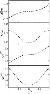
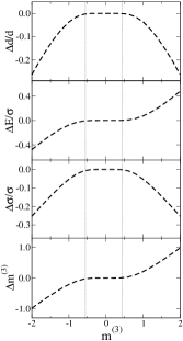
Figure 1: Moment discepancies in Cornish-Fisher (left) and continuous binomial (right) distributions. Each graph corresponds to the numerical moments compared with target moments, at different asymmetries $m^{(3)}$. The plots for Cornish-Fisher are with $m^{(4)}=3.0$ only; distributions with higher fourth moments show even larger discrepancies.

2. Binomial. The binomial distribution Zuker (2001) starts from the discrete expansion $(1+\lambda)^{N}=\sum{\lambda^{k}\left(\begin{array}[]{c}N\\ k\end{array}\right)}$. If the excitation energies come in discrete steps $\epsilon$, that is, $E_{x}=k\epsilon$, one can compute the moments for the discrete distribution exactly:

$$\bar{E}=\frac{N\epsilon\lambda}{1+\lambda}$$

$$\mu^{(2)}=\frac{N\epsilon^{2}\lambda}{(1+\lambda)^{2}}$$

$$m^{(3)}=\frac{1-\lambda}{\sqrt{N\lambda}}$$

$$m^{(4)}-3=\left(m^{(3)}\right)^{2}-\frac{2}{N}\;.$$ (11)

One can obtain a continuous distribution by using gamma functions:

$$\rho(E)=\lambda^{-E/\epsilon}\frac{\Gamma(E_{max}/\epsilon+1)}{\Gamma(E/\epsilon+1)\Gamma((E_{max}-E_{x})/\epsilon+1)}\;,$$ (12)

where $E_{\mathrm{max}}=N\epsilon$. The distribution can be shifted by adding a simple displacement $E_{\mathrm{min}}$ to the energy. The parameters $N,\lambda$ are fitted to the third moment and to either the total dimension $d=(1+\lambda)^{N}$ or, through rescaling, to the fourth moment.

In the limit of no asymmetry and $N\rightarrow\infty$ the binomial distribution goes to a Gaussian. The binomial distribution is positive-definite and has finite endpoints at ($E_{\mathrm{min}},N\epsilon+E_{\mathrm{min}}$). Unfortunately, once again, the relation between the parameters and the target moments, exact for the discrete distribution, is only approximate for the continuous distribution. We compared the discrepancy between target moments and numerical moment in the righthand side of Fig. 1. Once again, the approximate formulas (11) is restricted to $|m^{(3)}|<0.5$.

3. Modified Breit-Wigner (MBW). Given the problems with the previous models, we abandon generalizations of Gaussians and instead propose

$$\rho(E)=\frac{1}{W^{3}}\frac{(E-E_{min})^{2}(E_{max}-E)^{2}}{(E-E_{0})^{2}+W^{2}}$$ (13)

with endpoints given by $E_{\mathrm{min}},E_{\mathrm{max}}$. The first four moments can be computed analytically in terms of the four parameters; given target moments one can find the parameters by solving four nonlinear algebraic equations (plus an overall scale to match the correct dimension); we give the expressions in closed (but nontrivial) form in the Appendix. Unlike the Cornish-Fisher or binomial distributions, there is no discrepancy between the target and numerical moments.

The MBW distribution is applicable for

$$m^{(4)}-3>1.42\left(m^{(3)}\right)^{2}-0.52\;.$$ (14)

For third and fourth moments inside the allowed area, one can find real solutions for the MBW parameters. This region includes the numerically observed range for realistic interactions and model spaces Teran and Johnson (2006).

Table 1: Comparison of the moments reproduced by modified Breit-Wigner, Cornish-Fisher (C-F) and continuous binomial distributions. They are compared against exact calculations, all with GXPF1 interaction Honma et al. (2004) on pf-shell ⁴⁴Ti for the same three configurations shown in Fig. 2.

		target	C-F	Binomial
Part 100	E $\sigma$ $m^{(3)}$ $m^{(4)}$	-38.71 2.91 1.02 6.58	-38.76 2.87 1.26 6.87	-38.08 3.08 0.79 3.72
Part 079	E $\sigma$ $m^{(3)}$ $m^{(4)}$	-22.23 3.12 -0.70 5.43	-22.20 3.07 -0.61 3.59	-22.17 3.17 -0.62 3.36
Part 019	E $\sigma$ $m^{(3)}$ $m^{(4)}$	-27.39 3.30 -0.12 4.56	-27.39 3.30 -0.13 3.20	-27.39 3.30 -0.12 2.91

III.1 Direct comparison of model distributions

To facilitate comparison of the Cornish-Fisher, binomial, and MBW distributions, we make two side-by-side comparisons of these three models along with exact numerical configuration densities; specifically, we computed several partial densities for ⁴⁴Ti (2 protons and 2 neutrons in a $pf$-shell valence space) with the realistic interaction GXPF1 Honma et al. (2004), and chose to use three different configurations with different asymmetries $m^{(3)}$.

As discussed above, the “analytic” moments of the Cornish-Fisher and continuous binomial distribution are only approximate. Table 1 compares “exact” or target moments (shell-model calculations with REDSTICK code Ormand (2004)) and the numerical moments for the Cornish-Fisher and continuous binomial distributions. (The MBW numerical moments, as previously discussed, agree with the target moments.) The numerical Cornish-Fisher moments do well for centroids and widths, less well for $m^{(3)}$, and poorly for $m^{(4)}$; the continuous binomial has even larger errors.

One could in principle adjust the Cornish-Fisher or binomial parameters (with a different, or even an exact, parameterization) to get agreement between target and numerical moments, but this would have to be done numerically or through a look-up table. Furthermore, the binomial distribution has a much smaller region of applicability than the MBW distribution; one cannot find solutions for $|m^{(3)}|>0.5$.

In Fig. 2 we compare the MBW, Cornish-Fisher, and binomial distributions against realistic configuration densities from direct diagonalization using REDSTICK. Of the three models, the MBW appears to be better. Finally, we are able to compute the total level density with the MBW model for ⁴⁴Ti in the pf-shell with the GXPF1 interaction. Fig. 3 shows such calculation, and the exact calculation with the REDSTICK code, as well. In this example, the total level density is a sum of a 100 partial densities.

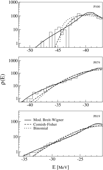
Figure 2: Representation of partial densities for three different configurations of ⁴⁴Ti in the pf-shell, with GXPF1 interaction. The modified Breit-Wigner, Cornish-Fisher and Binomial distributions are compared against the exact densities (solid plots with binned lines).

IV Summary

In order to invert configuration moments to get level densities, one must posit a model distribution whose parameters are fixed by the low-lying moments. An important consideration for modeling partial or configuration densities are model distributions that perform well for large asymmetries (third moments) which we have previously shown to be importantTeran and Johnson (2006). Continuing previous investigationV. K. B. Kota, V. Potbhare and P. Shenoy (1986), we have compared several distributions, in particular the Cornish-Fisher, continuous binomial, and a modified Breit-Wigner (MBW). We suggest that the MBW, or perhaps some variant, may be the most reliable for configuration densities, especially at large asymmetries.

V Acknowledgements

This work is supported by grant DE-FG52-03NA00082 from the Department of Energy.

Figure 3: Full ⁴⁴Ti level density in the pf-shell. The modeled level density (sum of MBW partial densities, broken line) is compared against the exact calculation (binned line).

*

Appendix A Moments expressions for the modified Breit-Wigner distribution

The modified Breit-Wigner distribution, with dimensions of [Energy]^-1, is

$$\rho(E)=\frac{1}{W^{3}}\frac{(E-E_{min})^{2}(E_{max}-E)^{2}}{(E-E_{0})^{2}+W^{2}},$$ (15)

defined on the interval $E_{\mathrm{min}}\leq E\leq E_{\mathrm{max}}$.

Define the dimensionless integrals

$$I_{0}(a,b)=\int_{a}^{b}\frac{1}{x^{2}+1}dx=\arctan b-\arctan a,$$ (16)

$$I_{1}(a,b)=\int_{a}^{b}\frac{x}{x^{2}+1}dx=\frac{1}{2}\ln\left(\frac{b^{2}+1}{a^{2}+1}\right).I_{n}(a,b)=\int_{a}^{b}\frac{x^{n}}{x^{2}+1}dx.$$ (17)

Also define the general integral (with an easily proved recursion relation),

$$I_{n}=\int_{a}^{b}\frac{x^{n}}{x^{2}+1}dx=\frac{1}{n-1}\left(b^{n-1}-a^{n-1}\right)-I_{n-2},$$ (18)

so that

$$I_{2n}=(-1)^{n}I_{0}+\sum_{k=1}^{n}\frac{(-1)^{n+k}}{2k-1}\left(b^{2k-1}-a^{2k-1}\right),$$ (19)

$$I_{2n+1}=(-1)^{n}I_{1}+\sum_{k=1}^{n}\frac{(-1)^{n+k}}{2k}\left(b^{2k}-a^{2k}\right).$$ (20)

Now introduce the convenient dimensionful integral

$$M_{n}=\int_{a}^{b}\left(E-E_{0}\right)^{n}\rho(E)dE.$$ (21)

We can write this in terms of the dimensionless integrals, using $a=(E_{\mathrm{min}}-E_{0})/W$ and $b=(E_{\mathrm{max}}-E_{0})/W$,

$$M_{n}=W^{n}\left(I_{n+4}-2(a+b)I_{n+3}+(a^{2}+4ab+b^{2})I_{n+2}-2(a+b)abI_{n+1}+a^{2}b^{2}I_{n}\right).$$ (22)

Finally, the moments in terms of the above expressions are

$$\text{dimension }D = \int_{a}^{b}\rho(E)dE=M_{0}$$ (23)

$$\text{centroid }\bar{E} = \int_{a}^{b}E\rho(E)dE=E_{0}+\frac{M_{1}}{M_{0}}=E_{0}+\Delta E$$ (24)

$$\text{variance }{\sigma}^{2} = \int_{a}^{b}(E-\bar{E})^{2}\rho(E)dE=\frac{1}{M_{0}}\left(M_{2}-2\Delta{E}M_{1}+\Delta{E}^{2}M_{0}\right)$$ (25)

$$m^{(3)} = \int_{a}^{b}(E-\bar{E})^{3}\rho(E)dE=\frac{1}{M_{0}{\sigma}^{3}}\left(M_{3}-3\Delta{E}M_{2}+3\Delta{E}^{2}M_{1}-\Delta{E}^{3}M_{0}\right)$$ (26)

$$m^{(4)} = \int_{a}^{b}(E-\bar{E})^{4}\rho(E)dE=\frac{1}{M_{0}{\sigma}^{4}}\left(M_{4}-4\Delta{E}M_{3}+6\Delta{E}^{2}M_{2}-4\Delta{E}^{3}M_{1}+\Delta{E}^{4}M_{0}\right).$$ (27)

References

- Hauser and Feshbach (1952) W. Hauser and H. Feshbach, Phys. Rev. 87, 366 (1952).
- T. Rauscher, F.-K. Thielemann and K.-L. Kratz (1997) T. Rauscher, F.-K. Thielemann and K.-L. Kratz, Phys. Rev. C 56, 1613 (1997).
- Griffin (1966) J. J. Griffin, Phys. Rev. Lett. 17, 478 (1966).
- B. Strohmaier, M. Fassbender and S. M. Qaim (1997) B. Strohmaier, M. Fassbender and S. M. Qaim, Phys. Rev. C 56, 2654 (1997).
- H. Feshbach, A. K. Kerman and S. E. Koonin (1980) H. Feshbach, A. K. Kerman and S. E. Koonin, Ann. Phys. 125, 429 (1980).
- Dean and Koonin (1999) D. J. Dean and S. E. Koonin, Phys. Rev. C 60, 054306 (1999).
- Ormand (1997) W. E. Ormand, Phys. Rev. C 56, R1678 (1997).
- B. Pichon (1994) B. Pichon, Nucl. Phys. A 568, 553 (1994).
- Goriely (1996) S. Goriely, Nucl. Phys. A 605, 28 (1996).
- P. Demetriou and S. Goriely (2001) P. Demetriou and S. Goriely, Nucl. Phys. A 695, 95 (2001).
- Nakada and Alhassid (1998) H. Nakada and Y. Alhassid, Phys. Lett. B 436, 231 (1998).
- Nakada and Alhassid (1997) H. Nakada and Y. Alhassid, Phys. Rev. Lett. 79, 2939 (1997).
- S. Hilaire (2004) S. Hilaire, Phys. Lett. B 583, 264 (2004).
- Y. Alhassid, G. F. Bertsch, and L. Fang (2003) Y. Alhassid, G. F. Bertsch, and L. Fang, Phys. Rev. C 68, 044322 (2003).
- M. Horoi, M. Ghita, and V. Zelevinsky (2004) M. Horoi, M. Ghita, and V. Zelevinsky, Phys. Rev. C 69, 041307 (2004).
- H. Nakamura and T. Fukahori (2005) H. Nakamura and T. Fukahori, Phys. Rev. C 72, 064329 (2005).
- C. W. Johnson, S. E. Koonin, G. H. Lang and W. E. Ormand (1995) C. W. Johnson, S. E. Koonin, G. H. Lang and W. E. Ormand, Phys. Rev. Lett. 69, 3157 (1995).
- D. J. Dean, S. E. Koonin, K. Langanke, P. B. Radha and Y. Alhassid (1995) D. J. Dean, S. E. Koonin, K. Langanke, P. B. Radha and Y. Alhassid, Phys. Rev. Lett. 74, 2909 (1995).
- G. H. Lang, C. W. Johnson, S. E. Koonin, and W. E. Ormand (1993) G. H. Lang, C. W. Johnson, S. E. Koonin, and W. E. Ormand, Phys. Rev. C 48, 1518 (1993).
- Y. Alhassid, D. J. Dean, S. E. Koonin, G. Lang, and W. E. Ormand (1994) Y. Alhassid, D. J. Dean, S. E. Koonin, G. Lang, and W. E. Ormand, Phys. Rev. Lett. 72, 613 (1994).
- S. E. Koonin, D. J. Dean, and K. Langanke (1997) S. E. Koonin, D. J. Dean, and K. Langanke, Phys. Rep. 278, 2 (1997).
- K. K. Mon and J. B. French (1975) K. K. Mon and J. B. French, Ann. Phys. 95, 90 (1975).
- Wong (1986) S. S. M. Wong, ed., Nuclear Statistical Spectroscopy (Oxford University Press, New York, 1986).
- V. K. B. Kota, V. Potbhare and P. Shenoy (1986) V. K. B. Kota, V. Potbhare and P. Shenoy, Phys. Rev. C 34, 2330 (1986).
- Horoi et al. (2003) M. Horoi, J. Kaiser, and V. Zelevinsky, Phys. Rev. C 67, 054309 (2003).
- J. B. French and K. F. Ratcliff (1971) J. B. French and K. F. Ratcliff, Phys. Rev. C 3, 94 (1971).
- S. Ayik and J.N. Ginocchio (1974) S. Ayik and J.N. Ginocchio, Nucl. Phys. A 221, 285 (1974).
- F. S. Chang and A. Zuker (1972) F. S. Chang and A. Zuker, Nucl. Phys. A p. 417 (1972).
- R. U. Haq and S. S. M. Wong (1979) R. U. Haq and S. S. M. Wong, Nucl. Phys. A 327, 314 (1979).
- M. R. Zirnbauer and D. M. Brink (1981) M. R. Zirnbauer and D. M. Brink, Z. Phys. A 301, 237 (1981).
- Agrawal and Kataria (1997) B. K. Agrawal and S. K. Kataria, Z. Phys. A 356, 369 (1997).
- Teran and Johnson (2006) E. Teran and C. W. Johnson, Phys. Rev. C 73, 024303 (2006).
- Zuker (2001) A. P. Zuker, Phys. Rev. C 64, 021303(R) (2001).
- Ormand (2004) W. E. Ormand (2004), private communication.
- H. Cramer (1946) H. Cramer, Mathematical Methods of Statistics (Princeton Univ. Press, Princeton, 1946).
- S. M. Grimes and T. N. Massey (1995) S. M. Grimes and T. N. Massey, Phys. Rev. C 51, 606 (1995).
- (37) T. N. Massey, private communication.
- Honma et al. (2004) M. Honma, T. Otsuka, B. A. Brown, and T. Mizusaki, Physical Review C 69, 034335 (2004).