Semileptonic Decays of Heavy Omega Baryons in a Quark Model

Abstract

JLAB-THY-06-480

I Introduction and Motivation

Semileptonic decay of hadrons are of interest for two basic reasons; they are the primary source of information for the extraction of the Cabbibo-Kobayashi-Maskawa (CKM) matrix elements of the Standard Model from experiment, and the study of the semileptonic decays of baryons provides information about their structure. In this manuscript, we present results of a calculation of the form factors and rates of the semileptonic decays of heavy $\Omega$ baryons ($\Omega_{Q}$) obtained using a constituent quark model. This work is similar to a recently published calculation of the semileptonic decays of heavy $\Lambda$ baryons MWS ($\Lambda_{Q}$) (hereinafter referred to as I). Although our motivation for the present work is similar, it is briefly recapitulated here for completeness.

The heavy quark effective theory (HQET) HQET has been a very powerful tool for the extraction of the CKM matrix elements from data on the semileptonic decay of mesons, especially for the decays of heavy mesons to heavy mesons where a number of relations that simplify this extraction are provided. For the semileptonic decays of a heavy baryon to another heavy baryon, HQET makes predictions that are analogous to those made for heavy-to-heavy meson decays: the six form factors that describe the decays to the ground-state heavy baryons are replaced by fewer form factors called Isgur-Wise functions; the normalization of at least one of these Isgur-Wise functions is known at the non-recoil point; corrections to this normalization first appear at order $1/m_{Q}^{2}$; and corrections can be systematically estimated in a $1/m_{Q}$ expansion. Note that for baryons, the number of Isgur-Wise functions needed at leading order depends on the flavor-spin structure of the parent and daughter baryons. For the semileptonic decays $\Omega_{Q}\to\Omega_{q}$, only two functions are required to describe the semileptonic decay in the heavy-quark limit. In the case of a heavy baryon decaying to a light baryon, HQET makes predictions that are not as powerful as in the heavy-to-heavy case. For example, for the semileptonic decays $\Omega_{Q}\to\Omega$, the leading-order HQET prediction is that the number of independent form factors decreases from six to four for a daughter $\Omega$ with spin 1/2.

While HQET has been tremendously successful and useful in treating the semileptonic decays of heavy hadrons, it has limitations. It is a limit of QCD that applies only to hadrons containing heavy quarks, and for the decays of such hadrons, it only predicts the relationships among form factors, not their kinematic dependence. In addition, the predictions of HQET are valid only as long as the energy of the daughter hadron is much smaller than the mass of the heavy quark. These limitations mean that the predictions of HQET must be augmented by information arising from other approaches to hadron structure.

While some work has been done in modeling the form factors for the semileptonic decays of heavy baryons, to the best of our knowledge little has been done in treating the decays to excited baryons. In I, the existing models of semileptonic decay in both meson and baryon sectors have been discussed. We have also outlined the procedure used to obtain the form factors and decay rates for semileptonic decay of $\Lambda_{Q}$ baryons using a non-relativistic quark model. Here we will focus only on the new aspects relevant to the semileptonic decay of $\Omega_{Q}$.

Very little theoretical or experimental work has been published to date on the semileptonic decay of $\Omega_{Q}$ baryons. Boyd and Brahm omegab1 have used HQET to show that the fourteen form factors that describe the decays $\Omega_{b}\to\Omega_{c}e\bar{\nu}$ and $\Omega_{b}\to\Omega_{c}^{*}(J^{P}=3/2^{+})e\bar{\nu}$ can be parametrized in terms of two nonperturbative functions at leading order, and in terms of five additional nonperturbative functions and one dimensional constant at order $1/m_{c}$. A $1/m_{c}$ expansion of the form factors for $\Omega_{b}\to\Omega_{c}^{(*)}$ has also been carried out by Sutherland omegab2 , who treated the effect of the $\Omega_{Q}^{*}-\Omega_{Q}$ mass splitting on the form factors evaluated at first order in $1/m_{c}$. A Bjorken sum rule for the semileptonic decays of $\Omega_{b}$ to the ground state and low-lying negative-parity excited-state charmed baryons has been derived by Xu omegab3 , again in the heavy quark limit. To the best of our knowledge, there are no calculations performed outside of the HQET framework, which motivates the present study.

There has recently been some progress in experiments dealing with these decays. The CLEO-c collaboration cleooc has published evidence for the observation of the decay $\Omega_{c}^{0}\to\Omega^{-}e^{+}\nu$, and have measured the product of the branching fraction and cross section to be $B(\Omega_{c}^{0}\to\Omega^{-}e^{+}\nu)\cdot\sigma(e^{+}e^{-}\to\Omega_{c}X)=42.2\pm 14.1\pm 11.9$ fb. The ARGUS argus and BELLE belle collaborations have also seen evidence for the $\Omega_{c}^{0}\to\Omega^{-}e^{+}\nu$ decay, but no quantitative value for the branching fraction has yet been published.

The procedure we follow here to calculate the form factors and rates for $\Omega_{Q}$ semileptonic decay is similar to that used for $\Lambda_{Q}$ decays in I. In a quark model context the flavor part of the $\Lambda_{Q}$ wave function is anti-symmetric under exchange of quarks 1 and 2, which comprise the light diquark system. This requires the spin-momentum part of the $\Lambda_{Q}$ wave function to be anti-symmetric under exchange of the two light quarks to maintain the appropriate Pauli exchange symmetry. On the other hand, $\Omega_{Q}$ baryons are described by a symmetric flavor wave function for the light diquark system. As a result, the spin-momentum part of the wave function has to be symmetric. This basic difference between the wave functions of $\Lambda_{Q}$ and $\Omega$ makes calculations of the form factors and the corresponding decay rates for their semileptonic decays significantly different.

This manuscript is organized as follows: in Section II we discuss the hadronic matrix elements and decay rates. Section III presents a brief outline of heavy quark effective theory as it relates to the $\Omega_{Q}$ decays that we discuss. In Section IV we describe the model we use to obtain the form factors, including some description of the Hamiltonian used to generate baryon wave functions. Our analytic results are discussed and compared to HQET results in Section V, our numerical results are given in Section VI, and Section VII presents our conclusions and an outlook. A number of details of the calculation, including the explicit expressions for the form factors, are shown in three Appendices.

II Matrix Elements and Decay Rates

The transition matrix element for the semileptonic decay $\Omega_{Q}\rightarrow\Omega_{q}\ell\nu_{\ell}$ is written

$$T=\frac{G_{F}}{\sqrt{2}}V_{Qq}\overline{u_{\ell}}\gamma^{\mu}(1-\gamma_{5})u_{\nu_{\ell}}\langle\Omega_{q}(p^{\prime},s^{\prime})|J_{\mu}|\Omega_{Q}(p,s)\rangle,$$ (1)

where $G_{F}/\sqrt{2}=g^{2}/(8M_{W}^{2})$ is the Fermi coupling constant, $M_{W}$ is the intermediate vector boson mass, $V_{Qq}$ is the CKM matrix element, $\overline{u_{\ell}}\gamma^{\mu}(1-\gamma_{5})u_{\nu_{\ell}}$ is the lepton current, and $J_{\mu}=\overline{q}\gamma_{\mu}(1-\gamma_{5})Q$ is the left handed current between quarks $Q$ and $q$. The hadronic matrix element of $J_{\mu}$ is described in terms of a number of form factors.

For transitions between ground state $(J^{P}=1/2^{+})$ baryons, the hadronic matrix elements of the vector ($V_{\mu}\equiv\overline{q}\gamma_{\mu}Q$) and axial ($A_{\mu}\equiv\overline{q}\gamma_{\mu}\gamma_{5}Q$) currents are

$$\langle B_{q}(p^{\prime},s^{\prime})|V_{\mu}|B_{Q}(p,s)\rangle=\overline{u}(p^{\prime},s^{\prime})\left(F_{1}(q^{2})\gamma_{\mu}+F_{2}(q^{2})\frac{p_{\mu}}{m_{B_{Q}}}+F_{3}(q^{2})\frac{p^{\prime}_{\mu}}{m_{B_{q}}}\right)u(p,s),$$ (2)

$$\langle B_{q}(p^{\prime},s^{\prime})|A_{\mu}|B_{Q}(p,s)\rangle=\overline{u}(p^{\prime},s^{\prime})\left(G_{1}(q^{2})\gamma_{\mu}+G_{2}(q^{2})\frac{p_{\mu}}{m_{B_{Q}}}+G_{3}(q^{2})\frac{p^{\prime}_{\mu}}{m_{B_{q}}}\right)\gamma_{5}u(p,s),$$ (3)

where the $F_{i}$ and $G_{i}$ are form factors which depend on the square of the momentum transfer $q=p-p^{\prime}$ between the initial and the final baryons. Similar expressions for transitions between $J^{P}=1/2^{+}$ ground states and final state baryons with other spins and parities are given in I. If $J\geq 3/2$ these expressions involve a fourth pair of form factors $F_{4}$ and $G_{4}$.

Expressions for the differential decay rates for semileptonic decays both including and ignoring the mass of the final leptons are given in I. These expressions can be integrated to yield the decay rates reported later in the present paper.

III Heavy Quark Effective Theory

In most applications of HQET, the aim has been to constrain the hadronic uncertainties in the extraction of CKM matrix elements such as $V_{ub}$ and $V_{cb}$. In this section, we take a different tack; we examine the predictions of HQET for decays of a heavy $\Omega$ into a number of the allowed excited heavy daughter baryons, with the aim of comparing these predictions with the form factors that we obtain in our model.

III.1 Structure of States and Parity Considerations

In a heavy excited baryon, the light quark system has some total angular momentum $j$, so that the total angular momentum of the baryon can be $J=j\pm 1/2$. These two states are degenerate because of the heavy quark spin symmetry. It is useful to show explicitly the representation we use for these two degenerate baryons. In the notation of Falk Falk , we write $u^{\mu_{1}\dots\mu_{j}}_{j+1/2}(v^{\prime})=u^{\mu_{1}\dots\mu_{j}}(v^{\prime})-u^{\mu_{1}\dots\mu_{j}}_{j-1/2}(v^{\prime})$, with

$$u^{\mu_{1}\dots\mu_{j}}(v^{\prime})=A^{\mu_{1}\dots\mu_{j}}(v^{\prime})u_{Q}(v^{\prime}).$$ (4)

Here, $u_{Q}(v)$ is the spinor of the heavy quark, with $v$ being the four-velocity and $A^{\mu_{1}\dots\mu_{j}}(v^{\prime})$ is a tensor that describes the spin-$j$ light quark system. This tensor is symmetric in all of its Lorentz indices, meaning that $u^{\mu_{1}\dots\mu_{j}}(v^{\prime})$ is also symmetric in all its Lorentz indices. Both $u^{\mu_{1}\dots\mu_{j}}_{j\pm 1/2}(v^{\prime})$ satisfy the conditions

$$v\hskip-5.0pt/^{\prime}u^{\mu_{1}\dots\mu_{j}}(v^{\prime}) = u^{\mu_{1}\dots\mu_{j}}(v^{\prime}),$$

$$v^{\prime}_{\mu_{i}}u^{\mu_{1}\dots\mu_{i}\dots\mu_{j}} = 0,\,\,g_{\mu_{k}\mu_{l}}{u}^{\mu_{1}\dots\mu_{j}}(v)=0,$$ (5)

where $\mu_{k}$ and $\mu_{l}$ indicate any pair of the indices $\mu_{1}\dots\mu_{j}$. The state with $J=j+1/2$ also satisfies

$$\gamma_{\mu_{i}}u^{\mu_{1}\dots\mu_{i}\dots\mu_{j}}_{j+1/2}=0.$$ (6)

Further details of the structure and properties of these tensors are given in Falk’s article Falk .

At this point, it is useful to discuss the parity of the states, which is determined by the parity of the light component. A spin-$j$ light quark component with parity $(-1)^{j}$ is said to have ‘natural’ parity, unnatural parity otherwise. The natural-parity light quark systems therefore have $j^{P}=(2n)^{+}$ or $j^{P}=(2n+1)^{-}$, with $n$ a positive integer or zero. The natural-parity light quark systems are represented by tensors, while those with unnatural parity are represented by pseudo-tensors. Since the parity of the baryon is that of the light quark system, we may refer to the baryons as being tensors or pseudo-tensors, with the understanding that this really refers to the light-quark component of the baryon. It is thus convenient to divide the decays we discuss into two classes, those in which the daughter baryons are tensors, and those in which they are pseudo-tensors.

III.2 Heavy to Heavy $\Omega$ Transitions

First, we note that the ground state of the $\Omega_{Q}$ has a symmetric flavor wave function for the light diquark, and so has a spin wave function that is also symmetric, corresponding to a total spin equal to one in the light quark component of the wave function. This state is therefore the spin-1/2 member of the lowest-lying $(1/2^{+},\,\,3/2^{+})$ multiplet. The Falk representation of this state is

$$\Omega_{\nu}(v)=\frac{1}{\sqrt{3}}\left(\gamma_{\nu}+v_{\nu}\right)\gamma_{5}u(v),$$ (7)

where $u(v)$ is a Dirac spinor. This state is a pseudotensor, and we begin with a discussion of decays to other pseudotensor states. We are interested in the matrix element

$${\cal A}=<\Omega_{c}^{(*)}(v^{\prime},j)|\bar{c}\Gamma b|\Omega_{b}(v)>,$$ (8)

where $c$ and $b$ are the heavy quark fields, and $\Gamma$ is an arbitrary combination of Dirac matrices. With the use of HQET, we may write this matrix element as

$$<\Omega_{c}^{(*)}(v^{\prime},j)|\bar{c}\Gamma b|\Omega_{b}(v)>=\bar{u}^{\mu_{1}\dots\mu_{j}}(v^{\prime})\Gamma\Omega^{\nu}M_{{\mu_{1}\dots\mu_{j}}\nu},$$ (9)

to leading order. Here, $M_{{\mu_{1}\dots\mu_{j}}\nu}$ is the most general tensor that we can construct, $\Omega^{\nu}$ is the Falk representation of Eq. (7), and $\bar{u}^{\mu_{1}\dots\mu_{j}}(v^{\prime})$ is the analogous representation of the daughter baryon. $M_{{\mu_{1}\dots\mu_{j}}\nu}$ may not contain any factors of $v^{\prime}_{\mu_{i}}$ or $g_{\mu_{i}\mu_{j}}$, and therefore takes the form

$$M_{{\mu_{1}\dots\mu_{j}}\nu}=\left(\eta_{1}^{(j)}g_{\mu_{1}\nu}+\eta_{2}^{(j)}v_{\mu_{1}}v^{\prime}_{\nu}\right)v_{\mu_{2}}\dots v_{\mu_{j}}.$$ (10)

Thus, two independent form factors, $\eta_{1,2}^{(j)}(v\cdot v^{\prime})$ are needed to this order, regardless of the spin of the final baryon.

Applying these results to the specific case of $j^{P}=0^{-}$, we find, for $J^{P}=1/2^{-}$

$$F_{1}=\frac{w-1}{\sqrt{3}}\eta^{(0)}_{2}(w),\,\,F_{2}=G_{2}=0,\,\,F_{3}=-G_{3}=\frac{2}{\sqrt{3}}\eta^{(0)}_{2}(w),\,\,G_{1}=\frac{w+1}{\sqrt{3}}\eta^{(0)}_{2}(w),$$ (11)

where $w=v\cdot v^{\prime}$. In this case, the daughter baryon is a singlet, and has no Lorentz indices. This means that the term in $g_{\mu\nu}$ is not present, and only the term in $\eta_{2}$ contributes to the matrix element.

When $j^{P}=1^{+}$, we find, for $J^{P}=1/2^{+},$

$$F_{1} = G_{1}=\frac{1}{3}\left[w\eta_{1}^{(1)}+\left(w^{2}-1\right)\eta_{2}^{(1)}\right],\,\,F_{2}=F_{3}=\frac{2}{3}\left[-\eta_{1}^{(1)}+\left(1-w\right)\eta_{2}^{(1)}\right],$$

$$G_{2} = -G_{3}=-\frac{2}{3}\left[\eta_{1}^{(1)}+\left(1+w\right)\eta_{2}^{(1)}\right],$$ (12)

and for $J^{P}=3/2^{+}$,

$$F_{1} = -\frac{1}{\sqrt{3}}\left[\eta_{1}^{(1)}+\left(w-1\right)\eta_{2}^{(1)}\right],\,\,F_{2}=G_{2}=0,\,\,F_{3}=-G_{3}=-\frac{2}{\sqrt{3}}\eta_{2}^{(1)},\,\,F_{4}=-G_{4}=-\frac{2}{\sqrt{3}}\eta_{1}^{(1)},$$

$$G_{1} = -\frac{1}{\sqrt{3}}\left[\eta_{1}^{(1)}+\left(w+1\right)\eta_{2}^{(1)}\right].$$ (13)

In these two sets of equations $\eta^{(1)}_{1,2}$ are two universal functions of the Isgur-Wise type. We note that there exist several multiplets that have the same quantum numbers as this ground state multiplet. The same is true in the case of $\Lambda_{Q}$ baryons, and these excited $\Lambda_{Q}$s were identified as radial excitations of the ground state. In the case of the $\Omega_{Q}$, such baryons are indeed excitations of the ground state, but they are not necessarily radial excitations. Some of these excitations are orbital excitations. However, independent of whether the daughter baryon belongs to the ground state $(1/2^{+},\,\,3/2^{+})$ or one of the excited multiplets, the expressions above for the form factors are valid. The explicit forms of the $\eta_{i}^{(1)}$ will depend on the details of the structure of the daughter baryon. For the ground state we know that at the non-recoil point, $\eta_{1}^{(1)}(v.v^{\prime}=1)=-1$, while the normalization of $\eta_{2}^{(1)}$ is not known. The negative sign of the normalization of $\eta_{1}^{(1)}$ arises because we have chosen a positive sign for the $g_{\mu_{1}\nu}$ term in Eq. (10).

For $j^{P}=2^{-}$, we find for $J^{P}=3/2^{-}$,

$$F_{1} = \frac{1}{\sqrt{30}}\left[(2w-1)\eta_{1}^{(2)}+2\left(w^{2}-1\right)\eta_{2}^{(2)}\right],\,\,F_{2}=-2\sqrt{\frac{2}{15}}\left[\eta_{1}^{(2)}+\left(w-1\right)\eta_{2}^{(2)}\right],$$

$$F_{3} = -\sqrt{\frac{2}{15}}\left[\eta_{1}^{(2)}+2\left(w-1\right)\eta_{2}^{(2)}\right],\,\,F_{4}=-\sqrt{\frac{2}{15}}(w-1)\eta_{1}^{(2)},$$

$$G_{1} = \frac{1}{\sqrt{30}}\left[(2w+1)\eta_{1}^{(2)}+2\left(w^{2}-1\right)\eta_{2}^{(2)}\right],\,\,G_{2}=-2\sqrt{\frac{2}{15}}\left[\eta_{1}^{(2)}+\left(w+1\right)\eta_{2}^{(2)}\right],$$

$$G_{3} = \sqrt{\frac{2}{15}}\left[\eta_{1}^{(2)}+2\left(w+1\right)\eta_{2}^{(2)}\right],\,\,G_{4}=\sqrt{\frac{2}{15}}(w+1)\eta_{1}^{(2)},$$ (14)

and for $J^{P}=5/2^{-}$,

$$F_{1} = -\frac{1}{\sqrt{3}}\left[\eta_{1}^{(2)}+\left(w-1\right)\eta_{2}^{(2)}\right],\,\,F_{2}=G_{2}=0,\,\,F_{3}=-G_{3}=-\frac{2}{\sqrt{3}}\eta_{2}^{(2)},\,\,F_{4}=-G4=-\frac{2}{\sqrt{3}}\eta_{1}^{(2)},$$

$$G_{1} = -\frac{1}{\sqrt{3}}\left[\eta_{1}^{(2)}+\left(w+1\right)\eta_{2}^{(2)}\right].$$ (15)

As with the previous example, the functions $\eta_{1,2}^{(2)}$ are Isgur-Wise form factors common to both decays.

For $j^{P}=3^{+}$, we find for $J^{P}=5/2^{+}$,

$$F_{1} = \frac{1}{3\sqrt{7}}\left[(3w-2)\eta_{1}^{(3)}+3\left(w^{2}-1\right)\eta_{2}^{(3)}\right],\,\,F_{2}=-2\sqrt{\frac{1}{7}}\left[\eta_{1}^{(3)}+\left(w-1\right)\eta_{2}^{(3)}\right],$$

$$F_{3} = -\frac{2}{3\sqrt{7}}\left[\eta_{1}^{(3)}+3\left(w-1\right)\eta_{2}^{(3)}\right],\,\,F_{4}=-\frac{4}{3\sqrt{7}}(w-1)\eta_{1}^{(3)},$$

$$G_{1} = \frac{1}{3\sqrt{7}}\left[(3w+2)\eta_{1}^{(3)}+3\left(w^{2}-1\right)\eta_{2}^{(3)}\right],\,\,G_{2}=-2\sqrt{\frac{1}{7}}\left[\eta_{1}^{(3)}+\left(w+1\right)\eta_{2}^{(3)}\right],$$

$$G_{3} = \frac{2}{3\sqrt{7}}\left[\eta_{1}^{(3)}+3\left(w+1\right)\eta_{2}^{(3)}\right],\,\,G_{4}=\frac{4}{3\sqrt{7}}(w+1)\eta_{1}^{(3)},$$ (16)

and for $J^{P}=7/2^{+}$,

$$F_{1} = -\frac{1}{\sqrt{3}}\left[\eta_{1}^{(3)}+\left(w-1\right)\eta_{2}^{(3)}\right],\,\,F_{2}=G_{2}=0,\,\,F_{3}=-G_{3}=-\frac{2}{\sqrt{3}}\eta_{2}^{(3)},\,\,F_{4}=-G_{4}=-\frac{2}{\sqrt{3}}\eta_{1}^{(3)},$$

$$G_{1} = -\frac{1}{\sqrt{3}}\left[\eta_{1}^{(3)}+\left(w+1\right)\eta_{2}^{(3)}\right]$$ (17)

The functions $\eta_{1,2}^{(3)}$ are Isgur-Wise form factors common to both decays. The normalizations of $\eta_{1,2}^{(2,3)}$ are not known.

For the tensor decays, the matrix element again takes the form shown in Eq. (9), but $M_{{\mu_{1}\dots\mu_{j}}\nu}$ must now be a pseudotensor. The only form that we can write is

$$M_{{\mu_{1}\dots\mu_{j}}\nu}=\tau^{(j)}(w)v_{\mu_{2}}\dots v_{\mu_{j}}\varepsilon_{\nu\mu_{1}\rho\lambda}v^{\rho}v^{\prime\lambda}.$$ (18)

When applied to the $1/2^{+}$ singlet daughter baryon, there is no way to create this pseudotensor, so such amplitudes vanish at leading order. For the other spin states, after some manipulation, we can express the form factors in terms of the set of Isgur-Wise functions $\tau^{(j)}(w)$.

For $j^{P}=1^{-}$, we find for the $1/2^{-}$ state

$$F_{1}=G_{1}=0,\,\,\,\,F_{2}=F_{3}=-G_{2}=G_{3}=-\frac{2}{3}\tau^{(1)},$$ (19)

while for $3/2^{-}$ state, the form factors are

$$F_{2}=G_{2}=0,\,G_{3}=-F_{3}=2F_{1}=-2G_{1}=-\frac{2}{\sqrt{3}}\tau^{(1)},\,F_{4}=-\frac{2}{\sqrt{3}}(w-1)\tau^{(1)},\,G_{4}=\frac{2}{\sqrt{3}}(w+1)\tau^{(1)}.$$ (20)

For $j^{P}=2^{+}$, starting with $3/2^{+}$, the form factors are

$$F_{1} = \frac{1}{\sqrt{30}}(1-w)\tau^{(2)},\,\,F_{2}=-G_{2}=-2\sqrt{\frac{2}{15}}\tau^{(2)},\,\,F_{3}=\sqrt{\frac{2}{15}}(w-2)\tau^{(2)},\,\,F_{4}=-G_{4}=\sqrt{\frac{2}{15}}(1-w^{2})\tau^{(2)},$$

$$G_{1} = \frac{1}{\sqrt{30}}(1+w)\tau^{(2)},\,\,G_{3}=-\sqrt{\frac{2}{15}}(w+2)\tau^{(2)}.$$ (21)

For the $5/2^{+}$ state, the form factors are

$$F_{2}=G_{2}=0,\,G_{3}=-F_{3}=2F_{1}=-2G_{1}=-\frac{2}{\sqrt{3}}\tau^{(2)},\,F_{4}=-\frac{2}{\sqrt{3}}(w-1)\tau^{(2)},\,G_{4}=\frac{2}{\sqrt{3}}(w+1)\tau^{(2)}.$$ (22)

The normalizations of none of the $\tau^{(i)}$ are known.

We do not present the predictions for the decays of $\Omega_{Q}$ to light $\Omega$ states, as the HQET predictions are not as useful as they are in the case of heavy to light $\Lambda_{Q}$ decays. For instance, the decays of the ground state $\Omega_{Q}$ to an $\Omega$ with $J^{P}=1/2^{+}$ are described in terms of four form factors in HQET, instead of six in general. While this small simplification is no doubt useful we do not pursue it here.

IV The Model

IV.1 Wave Function Components

In our model, a baryon state has the form

$$|A_{Q}({\bf p},s)\rangle = 3^{3/4}\int d^{3}p_{\rho}d^{3}p_{\lambda}C^{A}\Psi_{A_{Q}}^{S}|q_{1}({\bf p}_{1},s_{1})q_{2}({\bf p}_{2},s_{2})q_{3}({\bf p}_{3},s_{3})\rangle,$$

where ${\bf p}_{\rho}=\frac{1}{\sqrt{2}}({\bf p}_{1}-{\bf p}_{2})$ and ${\bf p}_{\lambda}=\frac{1}{\sqrt{6}}({\bf p}_{1}+{\bf p}_{2}-2{\bf p}_{3})$ are the Jacobi momenta, $C^{A}$ is the totally antisymmetric color wave function, and $\Psi_{A_{Q}}^{S}=\phi_{A_{Q}}\psi_{A_{Q}}\chi_{A_{Q}}$ is a symmetric combination of flavor, momentum and spin wave functions. The flavor wave functions of $\Omega_{Q}$ and $\Xi$ are

$$\phi_{\Omega_{Q}}=ssQ,\,\,\,\,\phi_{\Xi^{0}}=ssu,\,\,\,\,\phi_{\Xi^{-}}=ssd,$$

which are symmetric in quarks $1$ and $2$. The momentum-spin parts of the wave functions must therefore be symmetric in quarks $1$ and $2$ to keep the overall symmetry. The symmetric spin wave function $\chi_{3/2}^{S}$, and the mixed symmetric spin wave functions $\chi_{1/2}^{\rho}$, $\chi_{1/2}^{\lambda}$ are the usual eigenstates of total spin made of three spin-$1/2$ quarks.

The momentum wave function for total $L=\ell_{\rho}+\ell_{\lambda}$ is constructed from a Clebsch-Gordan sum of the wave functions of the two Jacobi momenta ${\bf p}_{\rho}$ and ${\bf p}_{\lambda}$, and takes the form

$$\psi_{LMn_{\rho}\ell_{\rho}n_{\lambda}\ell_{\lambda}}({\bf p}_{\rho},{\bf p}_{\lambda}) = \sum_{m}\langle LM|\ell_{\rho}m,\ell_{\lambda}M-m\rangle\psi_{n_{\rho}\ell_{\rho}m}({\bf p}_{\rho})\psi_{n_{\lambda}\ell_{\lambda}M-m}({\bf p}_{\lambda}).$$

The momentum and spin wave functions are then coupled to give symmetric wave functions corresponding to total spin $J$ and parity $(-1)^{(l_{\rho}+l_{\lambda})}$,

$$\Psi_{JM} = \sum_{M_{L}}\langle JM|LM_{L},SM-M_{L}\rangle\psi_{LM_{L}n_{\rho}\ell_{\rho}n_{\lambda}\ell_{\lambda}}({\bf p}_{\rho},{\bf p}_{\lambda})\chi_{S}(M-M_{L})$$ (23)

$$\equiv \left[\psi_{LM_{L}n_{\rho}\ell_{\rho}n_{\lambda}\ell_{\lambda}}({\bf p}_{\rho},{\bf p}_{\lambda})\chi_{S}(M-M_{L})\right]_{J,M}.$$

The full wave function for a state $A$ is built from a linear superposition of such components as

$$\Psi_{A,J^{P}M}=\phi_{A}\sum_{i}\eta_{i}^{A}\Psi_{JM}^{i}.$$ (24)

Here $\phi_{A}$ is the flavor wave function of the state $A$, and the $\eta_{i}^{A}$ are coefficients that are determined by diagonalizing a Hamiltonian in the basis of the $\Psi_{JM}^{i}$. For this calculation, we limit the expansion in the last equation to components that satisfy $N\leq 2$, where $N=2(n_{\rho}+n_{\lambda})+\ell_{\rho}+\ell_{\lambda}.$ Consistent with this is the fact that the states we discuss all correspond to $N\leq 2$.

The wave functions for $\Omega_{Q}$ with $J^{P}=1/2^{+}$ have the form

$$\Psi^{\Omega_{Q}}_{1/2^{+}M} = \phi_{\Omega_{Q}}\left(\vphantom{\sum_{i}}\left[\eta_{1}^{\Omega_{Q}}\psi_{000000}({\bf p}_{\rho},{\bf p}_{\lambda})+\eta_{2}^{\Omega_{Q}}\psi_{001000}({\bf p}_{\rho},{\bf p}_{\lambda})+\eta_{3}^{\Omega_{Q}}\psi_{000010}({\bf p}_{\rho},{\bf p}_{\lambda})\right]\chi_{1/2}^{\lambda}(M)\right.$$ (25)

$$+ \eta_{4}^{\Omega_{Q}}\psi_{000101}({\bf p}_{\rho},{\bf p}_{\lambda})\chi_{1/2}^{\rho}(M)+\eta_{5}^{\Omega_{Q}}\left[\psi_{1M_{L}0101}({\bf p}_{\rho},{\bf p}_{\lambda})\chi_{1/2}^{\rho}(M-M_{L})\right]_{1/2,M}$$

$$+ \eta_{6}^{\Omega_{Q}}\left[\psi_{2M_{L}0200}({\bf p}_{\rho},{\bf p}_{\lambda})\chi_{3/2}^{S}(M-M_{L})\right]_{1/2,M}$$

$$+ \left.\eta_{7}^{\Omega_{Q}}\left[\psi_{2M_{L}0002}({\bf p}_{\rho},{\bf p}_{\lambda})\chi_{3/2}^{S}(M-M_{L})\right]_{1/2,M}\right).$$

The complete expressions for $\Omega_{Q}$ wave functions of different spins and parities are given in Appendix A. A simplified version of the model would truncate the expansion of the wave functions, giving

$$\Psi_{\Omega_{Q},1/2^{+}M}=\phi_{\Omega}\psi_{000000}({\bf p}_{\rho},{\bf p}_{\lambda})\chi_{1/2}^{\lambda}(M)$$ (26)

for the ground state. There are a number of daughter baryons that have an overlap with the ground state $\Omega_{Q}$ (in the spectator approximation that we use), even when we limit the discussion to states with $N\leq 2$. There are three states with $J^{P}=1/2^{+}$, two with $J^{P}=1/2^{-}$, two with $J^{P}=3/2^{-}$, four with $J^{P}=3/2^{+}$, one with $J^{P}=5/2^{-}$, two with $J^{P}=5/2^{+}$, and one with $J^{P}=7/2^{+}$, all of which occur in the $N\leq 2$ bands. The single-component representations of these states are

$$\Psi_{\Omega_{Q},1/2^{+}M} = \phi_{\Omega}\psi_{000000}({\bf p}_{\rho},{\bf p}_{\lambda})\chi_{1/2}^{\lambda}(M),$$

$$\Psi_{\Omega_{Q},1/2^{+}_{1}M} = \phi_{\Omega}\psi_{000010}({\bf p}_{\rho},{\bf p}_{\lambda})\chi_{1/2}^{\lambda}(M),$$

$$\Psi_{\Omega_{Q},1/2^{+}_{2}M} = \phi_{\Omega}[\psi_{2M_{L}0002}({\bf p}_{\rho},{\bf p}_{\lambda})\chi_{3/2}^{S}(M-M_{L})]_{1/2,M},$$

$$\Psi_{\Omega_{Q},1/2^{-}M} = \phi_{\Omega}[\psi_{1M_{L}0001}({\bf p}_{\rho},{\bf p}_{\lambda})\chi_{1/2}^{\lambda}(M-M_{L})]_{1/2,M},$$

$$\Psi_{\Omega_{Q},1/2^{-}_{1}M} = \phi_{\Omega}[\psi_{1M_{L}0001}({\bf p}_{\rho},{\bf p}_{\lambda})\chi_{3/2}^{S}(M-M_{L})]_{1/2,M},$$

$$\Psi_{\Omega_{Q},3/2^{-}M} = \phi_{\Omega}[\psi_{1M_{L}0001}({\bf p}_{\rho},{\bf p}_{\lambda})\chi_{1/2}^{\lambda}(M-M_{L})]_{3/2,M},$$

$$\Psi_{\Omega_{Q},3/2^{-}_{1}M} = \phi_{\Omega}[\psi_{1M_{L}0001}({\bf p}_{\rho},{\bf p}_{\lambda})\chi_{3/2}^{S}(M-M_{L})]_{3/2,M},$$

$$\Psi_{\Omega_{Q},5/2^{-}M} = \phi_{\Omega}[\psi_{1M_{L}0001}({\bf p}_{\rho},{\bf p}_{\lambda})\chi_{3/2}^{S}(M-M_{L})]_{5/2,M},$$

$$\Psi_{\Omega_{Q},3/2^{+}M} = \phi_{\Omega}\psi_{000000}({\bf p}_{\rho},{\bf p}_{\lambda})\chi_{3/2}^{S}(M),$$

$$\Psi_{\Omega_{Q},3/2^{+}_{1}M} = \phi_{\Omega}\psi_{000010}({\bf p}_{\rho},{\bf p}_{\lambda})\chi_{3/2}^{S}(M),$$

$$\Psi_{\Omega_{Q},3/2^{+}_{2}M} = \phi_{\Omega}[\psi_{2M_{L}0002}({\bf p}_{\rho},{\bf p}_{\lambda})\chi_{3/2}^{S}(M-M_{L})]_{3/2,M},$$

$$\Psi_{\Omega_{Q},3/2^{+}_{3}M} = \phi_{\Omega}[\psi_{2M_{L}0002}({\bf p}_{\rho},{\bf p}_{\lambda})\chi_{1/2}^{\lambda}(M-M_{L})]_{3/2,M},$$

$$\Psi_{\Omega_{Q},5/2^{+}M} = \phi_{\Omega}[\psi_{2M_{L}0002}({\bf p}_{\rho},{\bf p}_{\lambda})\chi_{1/2}^{\lambda}(M-M_{L})]_{5/2,M},$$

$$\Psi_{\Omega_{Q},5/2^{+}_{1}M} = \phi_{\Omega}[\psi_{2M_{L}0002}({\bf p}_{\rho},{\bf p}_{\lambda})\chi_{3/2}^{S}(M-M_{L})]_{5/2,M},$$

$$\Psi_{\Omega_{Q},7/2^{+}M} = \phi_{\Omega}[\psi_{2M_{L}0002}({\bf p}_{\rho},{\bf p}_{\lambda})\chi_{3/2}^{S}(M-M_{L})]_{7/2,M}.$$ (27)

A common choice for constructing baryon wave function is the harmonic oscillator basis. One advantage of using this basis is that it facilitates calculation of the required matrix elements. However, it leads to form factors that fall off too rapidly at large values of momentum transfer. We therefore also use the so-called Sturmian basis KP . In this basis, form factors have multipole dependence on $q^{2}$, which is what is expected experimentally.

The explicit wave functions in momentum space are

$$\psi^{\rm h.o.}_{nLm}({\bf p}) = \left[\frac{2\,n!}{\left(n+L+{\textstyle{1\over 2}}\right)!}\right]^{{\textstyle{1\over 2}}}(i)^{L}(-1)^{n}\frac{1}{\alpha^{L+{\textstyle{3\over 2}}}}e^{-\frac{p^{2}}{(2\alpha^{2})}}L_{n}^{L+{\textstyle{1\over 2}}}(p^{2}/\alpha^{2}){\cal Y}_{Lm}({\bf p})$$ (28)

in the harmonic oscillator basis, and

$$\psi^{\rm St}_{nLm}({\bf p}) = {2\left[n!(n+2L+2)!\right]^{{\textstyle{1\over 2}}}\over\left(n+L+{\textstyle{1\over 2}}\right)!}(i)^{L}\frac{1}{\beta^{L+{\textstyle{3\over 2}}}}\frac{1}{\left(\frac{p^{2}}{\beta^{2}}+1\right)^{L+2}}P_{n}^{\left(L+{\textstyle{3\over 2}},L+{\textstyle{1\over 2}}\right)}\left(\frac{p^{2}-\beta^{2}}{p^{2}+\beta^{2}}\right){\cal Y}_{Lm}({\bf p})$$

in the Sturmian basis. The $L_{n}^{\nu}(x)$ are generalized Laguerre polynomials and the $P_{n}^{(\mu,\nu)}(y)$ are Jacobi polynomials, with $p=\left|{\bf p}\right|$.

IV.2 Hamiltonian

The phenomenological Hamiltonian we use has the form

$$H=\sum_{i=1}^{3}K_{i}+C_{qqq}+\sum_{i<j=1}^{3}\left({br_{ij}\over 2}-{2\alpha_{\rm Coul}\over 3r_{ij}}+{2\alpha_{\rm hyp}\over 3m_{i}m_{j}}{8\pi\over 3}{\bf S}_{i}\cdot{\bf S}_{j}\delta^{3}({\bf r}_{ij})\right),$$ (30)

with $r_{ij}=|{\bf r}_{i}-{\bf r}_{j}|$. The spin independent confining potential consists of a linear and a Coulomb component, and the spin-dependent part of the potential takes the form of a contact hyperfine interaction. Spin-orbit and tensor interactions are neglected. We note here that $\alpha_{\rm Coul}$, $\alpha_{\rm hyp}$, $b$, $C_{qqq}$, and $m_{i}$ are not fundamental, but are phenomenological parameters obtained from a fit to the spectrum of baryon states. In the sum $\sum_{i=1}^{3}K_{i}$ of the kinetic energies of the quarks, each term has either the usual non-relativistic form given by

$$K_{i}=\left(m_{i}+\frac{p_{i}^{2}}{2m_{i}}\right),$$ (31)

or a semi-relativistic form given by

$$K_{i}=\sqrt{p_{i}^{2}+m_{i}^{2}}.$$ (32)

IV.3 Obtaining the Form Factors

IV.3.1 $\Omega_{Q}\to\Omega_{q}$

Here, we illustrate the procedure we follow to obtain the form factors, using the decay of the $B_{Q}$ to the ground state $B_{q}$ as an example. We note here that $B_{Q}$ represents $\Omega_{Q}$ and $B_{q}$ refers to any of the $\Omega_{q}$ or $\Xi$ in their ground state. We show the procedure only for the vector current matrix element from Eq. (2), with the assumption that the parent $B_{Q}$ is at rest and the daughter $B_{q}$ has three momentum ${\bf p}$. The left-hand side of Eq. (2) is evaluated using the quark model, after the operator $V_{\mu}=\bar{q}\gamma_{\mu}Q$ has been reduced to its Pauli (non-relativistic) form. Specific values for the index $\mu$ are chosen, as well as specific values of $s$ and $s^{\prime}$. By making three sets of such choices, three equations for the $F_{i}$ in terms of the quark-model matrix elements of three operators are obtained. This system of equations is then solved to obtain the expressions for the form factors. In the specific case at hand, choosing $s=s^{\prime}=+1/2$ and $\mu=0$, for instance, leads to

$$\langle B_{q}({\bf p},+)|\bar{q}\gamma_{0}Q|B_{Q}(0,+)\rangle = \int d^{3}p^{\prime}_{\rho}d^{3}p^{\prime}_{\lambda}d^{3}p_{\rho}d^{3}p_{\lambda}C^{A*}C^{A}\Psi_{B_{q}}^{*S}(+)$$

$$\times \langle q^{\prime}_{1}q^{\prime}_{2}q|q^{\dagger}\gamma_{0}Q|q_{1}q_{2}Q\rangle\Psi_{B_{Q}}^{S}(+).$$

where

$$\langle q^{\prime}_{1}q^{\prime}_{2}q|q^{\dagger}\gamma_{0}Q|q_{1}q_{2}Q\rangle=\langle q^{\prime}_{1}q^{\prime}_{2}|q_{1}q_{2}\rangle\langle q|q^{\dagger}\gamma_{0}Q|Q\rangle.$$

The matrix element $\langle q^{\prime}_{1}q^{\prime}_{2}|q_{1}q_{2}\rangle$ gives $\delta$-functions in spin, momentum and flavor in the spectator approximation. Using the $\delta$-functions in momentum and flavor, the integral simplifies to

$$\left<B_{q}({\bf p},+)\left|{\cal O}_{0}\right|B_{Q}({\bf 0},+)\right> = \int d^{3}p_{\rho}d^{3}p_{\lambda}\psi_{B_{q}}^{*}({\bf p}^{\prime}_{\rho},{\bf p}^{\prime}_{\lambda}){\cal A}^{++}_{B_{Q}B_{q}}({\cal O}_{0})\psi_{B_{Q}}({\bf p}_{\rho},{\bf p}_{\lambda}),$$ (34)

with ${\bf p}^{\prime}_{\rho}={\bf p}_{\rho}$, ${\bf p}^{\prime}_{\lambda}={\bf p}_{\lambda}-2\sqrt{3/2}\,m_{\sigma}{\bf p}/m_{B_{q}}$, where $m_{\sigma}$ is the mass of the light quark and ${\cal O}_{0}=q^{\dagger}\gamma_{0}Q$. It is useful for us to define

$${\cal A}^{s^{\prime}s}_{B_{Q}B_{q}}({\cal O}_{\mu}) = \chi_{B_{q}}^{\dagger}(s^{\prime})\delta_{s^{\prime}_{1}s_{1}}\delta_{s^{\prime}_{2}s_{2}}\langle q({\bf p}^{\prime}_{3},s^{\prime}_{3})\left|{\cal O}_{\mu}\right|Q({\bf p}_{3},s_{3})\rangle\chi_{B_{Q}}(s).$$ (35)

where ${\bf p}^{\prime}_{3}={\bf p}-\sqrt{\frac{2}{3}}{\bf p}_{\lambda}$ and ${\bf p}_{3}=-\sqrt{\frac{2}{3}}{\bf p}_{\lambda}$. We have

$${\cal A}^{++}_{B_{Q}B_{q}}({\cal O}_{\mu})=\frac{1}{3}\langle q({\bf p}^{\prime}_{3},\uparrow)\left|{\cal O}_{\mu}\right|Q({\bf p}_{3},\uparrow)\rangle+\frac{2}{3}\langle q({\bf p}^{\prime}_{3},\downarrow)\left|{\cal O}_{\mu}\right|Q({\bf p}_{3},\downarrow)\rangle,$$ (36)

where both parent and daughter baryons are in the ground state.

After the spin matrix elements are evaluated, the momentum integrals are performed using both bases for the momentum wave functions shown earlier. The analytic results for the form factors for the $\Omega_{Q}\to\Omega_{q}$ decays, evaluated using the truncated basis of Eq. (IV.1), are given in Appendix B. For decays to excited states, the calculation of the form factors is a little more involved, but the basic idea is as outlined here.

IV.3.2 $\Omega_{c}\to\Omega^{(*)}$

The calculation of form factors for $\Omega_{c}\to\Omega^{(*)}$ decays is similar to that described above, up to a question of symmetry. The flavor wave functions of $\Omega_{c}$ and $\Omega$ are $\phi_{\Omega_{c}}=ssc$ and $\phi_{\Omega}=sss$. In a semileptonic decay process the charm quark of the $\Omega_{c}$ decays into an $s$ quark, which can be any of the three $s$ quarks of the $\Omega$. Thus, we need to evaluate

$$\frac{1}{\sqrt{3}}\left(\vphantom{\frac{1}{\sqrt{3}}}\langle\Omega({\bf p},+)|{\cal O}_{\mu}|\Omega_{Q}({\bf 0},+)\rangle+\langle\Omega({\bf p},+)|\{13\}{\cal O}_{\mu}|\Omega_{Q}({\bf 0},+)\rangle+\langle\Omega({\bf p},+)|\{23\}{\cal O}_{\mu}|\Omega_{Q}({\bf 0},+)\rangle\right).$$

The factor $\frac{1}{\sqrt{3}}$ comes from the normalization. The wave functions for the $\Omega$ states are fully symmetric under interchange of any of the quarks, so each of the permuted matrix elements reproduces the one without permutations. The result is that we must calculate

$$\sqrt{3}\langle\Omega({\bf p},+)|{\cal O}_{\mu}|\Omega_{Q}({\bf 0},+)\rangle,$$

to obtain the form factors for $\Omega_{c}\to\Omega$.

The procedure described in this subsection is relatively straightforward to implement in the harmonic oscillator basis, largely due to the fact that the Moshinsky rotations have been treated by a number of authors, and are also fairly simple to calculate. In particular, the fact that the ‘permuted’ wave function can be written in terms of a finite set of transformed wave function components is another feature that makes the harmonic oscillator basis attractive for calculations like these. In the Sturmian basis, however, the permutation of particles requires an infinite sum of transformed wave functions. This sum could be truncated at some point in a calculation such as this. However, at this point we do not examine decays to daughter $\Omega$’s in the Sturmian basis.

V Analytic Results and Comparison with HQET

The analytic expressions that we obtain for the form factors are shown in Appendix B, for both the Sturmian and harmonic oscillator bases. The results shown there are valid when the wave function for a particular state is written as a single component, in either expansion basis. As mentioned earlier, one of the advantages of the Sturmian basis is that it leads to form factors that behave like multipoles in the kinematic variable, and this is seen in the forms that we display.

At this point, it is instructive to compare, as far as possible, these analytic forms with the predictions of HQET. While HQET does not give the explicit forms of the form factors, a number of relationships among the form factors are expected, and any model should reproduce these relationships. In what follows, we restrict our comparison to the predictions that are valid at the non-recoil point, as we have ignored any kinematic dependence beyond the Gaussian or multipole factors shown in Appendix B. In addition, we focus on the predictions for heavy to heavy transitions.

The quark model states we use are constructed in the coupling scheme

$$|J^{P},L,S>=\left|\left[\left(\ell_{\rho}\ell_{\lambda}\right)_{L}\left(s_{12}s_{3}\right)_{S}\right]_{J}\right>,$$ (37)

where the notation $(ab)_{c}$ means angular momentum $c$ is formed by vector addition from angular momenta $a$ and $b$. The parity $P$ is $(-1)^{\ell_{\rho}+\ell_{\lambda}}$, the total spin of the two light quarks in the baryon is $s_{12}$, and $s_{3}$ is the spin of the third quark, taken to be the heavy quark.

The HQET states are assumed to have the coupling scheme

$$|J^{P},j>=\left|\left\{\left[\left(\ell_{\rho}\ell_{\lambda}\right)_{L}s_{12}\right]_{j}s_{3}\right\}_{J}\right>,$$ (38)

where $j$ is the total spin of the light component of the baryon, so that $J=j\pm 1/2$. The states of one coupling scheme are linear combinations of the states of the second. In particular, we find

$$\left|\left\{\left[\left(\ell_{\rho}\ell_{\lambda}\right)_{L}s_{12}\right]_{j}s_{3}\right\}_{J}\right>=(-1)^{1/2+s_{12}+L+J}\sqrt{2j+1}$$

$$\times\sum_{S}\sqrt{2S+1}\left\{\begin{array}[]{ccc}1/2&s_{12}&S\\ L&J&j\end{array}\right\}\left|\left[\left(\ell_{\rho}\ell_{\lambda}\right)_{L}\left(s_{12}s_{3}\right)_{S}\right]_{J}\right>,$$ (41)

where $\left\{\begin{array}[]{ccc}1/2&s_{12}&S\\ L&J&j\end{array}\right\}$ is a 6-J symbol.

For the states that we consider, the explicit expressions for the HQET states in terms of the quark model states are

$$\left|1/2^{-},j=1\right> = \sqrt{\frac{2}{3}}\left|1/2^{-},L=1,S=1/2\right>+\frac{1}{\sqrt{3}}\left|1/2^{-},L=1,S=3/2\right>,$$

$$\left|1/2^{-},j=0\right> = -\frac{1}{\sqrt{3}}\left|1/2^{-},L=1,S=1/2\right>+\sqrt{\frac{2}{3}}\left|1/2^{-},L=1,S=3/2\right>,$$

$$\left|3/2^{-},j=2\right> = \sqrt{\frac{5}{6}}\left|3/2^{-},L=1,S=1/2\right>+\frac{1}{\sqrt{6}}\left|3/2^{-},L=1,S=3/2\right>,$$

$$\left|3/2^{-},j=1\right> = -\frac{1}{\sqrt{6}}\left|3/2^{-},L=1,S=1/2\right>+\sqrt{\frac{5}{6}}\left|3/2^{-},L=1,S=3/2\right>,$$

$$\left|3/2^{+},j=2\right> = \frac{1}{\sqrt{2}}\left(\left|3/2^{+},L=2,S=1/2\right>+\left|3/2^{+},L=2,S=3/2\right>\right),$$

$$\left|3/2^{+},j=1\right> = \frac{1}{\sqrt{2}}\left(-\left|3/2^{+},L=2,S=1/2\right>+\left|3/2^{+},L=2,S=3/2\right>\right),$$

$$\left|5/2^{+},j=3\right> = \frac{\sqrt{7}}{3}\left|5/2^{+},L=2,S=1/2\right>+\frac{\sqrt{2}}{3}\left|5/2^{+},L=2,S=3/2\right>,$$

$$\left|5/2^{+},j=2\right> = -\frac{\sqrt{2}}{3}\left|5/2^{+},L=2,S=1/2\right>+\frac{\sqrt{7}}{3}\left|5/2^{+},L=2,S=3/2\right>.$$ (42)

For all of the quark model states shown on the r.h.s of these equations, $S=1/2$ corresponds to spin wave function of the $\chi^{\lambda}$ type. The form factors that describe transitions to these states are shown in Appendix C.

Other states not shown above are single component states in both representations, and these are

$$\left|1/2^{+},j=1\right> = \left|1/2^{+},L=0,S=1/2\right>,$$

$$\left|3/2^{+},j=1\right> = \left|3/2^{+},L=0,S=3/2\right>,$$

$$\left|1/2^{+}_{1},j=1\right> = \left|1/2^{+}_{1},L=0,S=1/2\right>,$$

$$\left|3/2^{+}_{1},j=1\right> = \left|3/2^{+}_{1},L=0,S=3/2\right>,$$

$$\left|1/2^{+}_{2},j=1\right> = \left|1/2^{+}_{2},L=2,S=3/2\right>,$$

$$\left|5/2^{-},j=2\right> = \left|5/2^{-},L=1,S=3/2\right>.$$ (43)

The subscripts ‘1’ denotes the first radially-excited copy of the ground state multiplet. The ‘2’ denotes an orbitally-excited state with $J^{P}=1/2^{+}$. This state forms a $j=1$ multiplet with the second $3/2^{+}$ state listed in Eq. (V).

We now examine the form factors of Appendix C, along with some of the form factors in Appendix B, and compare these with the predictions of HQET shown in Section III.2. We begin with a discussion of the decays to pseudotensor final states.

V.1 $1/2^{-}$

The HQET predictions for decays to this state are shown in Eq. (11), while the quark model form factors are shown in Section C.1. Noting that $w-1\approx{\cal O}\left(1/m_{q}\right)$, the leading order predictions are that $F_{1}=F_{2}=G_{2}=0$, and $F_{3}=-G_{3}=G_{1}$. The form factors of Section C.1 satisfy these relations, and allow us to identify

$$\eta_{2}^{(0)}=\frac{m_{\sigma}}{\alpha_{\lambda}}\left(\frac{\alpha_{\lambda}\alpha_{\lambda^{\prime}}}{\alpha_{\lambda\lambda^{\prime}}^{2}}\right)^{5/2}\exp\left(-\frac{3m^{2}_{\sigma}}{2m^{2}_{\Omega_{q}}}\frac{p^{2}}{\alpha_{\lambda\lambda^{\prime}}^{2}}\right),$$

in the harmonic oscillator models, or

$$\eta_{2}^{(0)}=\frac{m_{\sigma}}{\beta_{\lambda}}\sqrt{2}\frac{\left(\frac{\beta_{\lambda}\beta_{\lambda^{\prime}}}{\beta_{\lambda\lambda^{\prime}}^{2}}\right)^{5/2}}{\left[1+\frac{3}{2}\frac{m^{2}_{\sigma}}{m^{2}_{\Omega_{q}}}\frac{p^{2}}{\beta_{\lambda\lambda^{\prime}}^{2}}\right]^{3}}$$ (44)

in the Sturmian models. In these expressions, and in those that follow,

$$\alpha_{\lambda\lambda^{\prime}}^{2}=\frac{1}{2}(\alpha_{\lambda}^{2}+\alpha_{\lambda^{\prime}}^{2})$$ (45)

and

$$\beta_{\lambda\lambda^{\prime}}=\frac{1}{2}(\beta_{\lambda}+\beta_{\lambda}^{\prime}).$$ (46)

V.2 $(1/2^{+},\,\,3/2^{+})$

The HQET predictions for decays to this pair of states are shown in Eqs. (III.2) and (III.2). The three multiplets with these quantum numbers are discussed separately.

V.2.1 Ground State

The quark model form factors for the ground state doublet are shown in Sections B.1 and B.8. Comparison of these form factors with the predictions of HQET leads to

$$\eta_{2}^{(1)}=-\frac{1}{2}\eta_{1}^{(1)}$$ (47)

at the non-recoil point, and allows us to identify

$$\eta_{1}^{(1)}=-\left(\frac{\alpha_{\lambda}\alpha_{\lambda^{\prime}}}{\alpha_{\lambda\lambda^{\prime}}^{2}}\right)^{3/2}\exp\left(-\frac{3m^{2}_{\sigma}}{2m^{2}_{\Omega_{q}}}\frac{p^{2}}{\alpha_{\lambda\lambda^{\prime}}^{2}}\right),$$ (48)

in the harmonic oscillator models, or

$$\eta_{1}^{(1)}=-\frac{\left(\frac{\beta_{\lambda}\beta_{\lambda^{\prime}}}{\beta_{\lambda\lambda^{\prime}}^{2}}\right)^{3/2}}{\left[1+\frac{3}{2}\frac{m^{2}_{\sigma}}{m^{2}_{\Omega_{q}}}\frac{p^{2}}{\beta_{\lambda\lambda^{\prime}}^{2}}\right]^{3}}$$ (49)

in the Sturmian models. In the heavy quark limit, both forms yield the expected normalization at the non-recoil point, namely $\eta_{1}^{(1)}(w=1)=-1$. It must be emphasized that the relationship between $\eta_{1}^{(1)}$ and $\eta_{2}^{(1)}$ given above is one that arises only in the context of the quark model. In HQET, these two Isgur-Wise functions are a priori independent of each other. A more complete expression of the relationship between $\eta_{1}^{(1)}$ and $\eta_{2}^{(1)}$ can be obtained by noting that $G_{2}$ and $G_{3}$ for the $1/2^{+}$ final state both vanish at leading order in the quark model. This leads to

$$\eta_{1}^{(1)}(w)=-(1+w)\eta_{2}^{(1)}(w),$$ (50)

valid at leading order in the heavy quark expansion.

V.2.2 Radial Excitation

The form factors for decays to the radially excited $(1/2^{+},\,\,3/2^{+})$ multiplet are shown in Sections B.2 and B.9. Comparison of these form factors with the predictions of HQET again leads to

$$\eta_{2}^{(1)}=-\frac{1}{2}\eta_{1}^{(1)},$$ (51)

and allows us to identify

$$\eta_{1}^{(1)}=\sqrt{\frac{3}{8}}\frac{\alpha_{\lambda}^{2}-\alpha_{\lambda^{\prime}}^{2}}{\alpha_{\lambda}\alpha_{\lambda^{\prime}}}\left(\frac{\alpha_{\lambda}\alpha_{\lambda^{\prime}}}{\alpha_{\lambda\lambda^{\prime}}^{2}}\right)^{5/2}\exp\left(-\frac{3m^{2}_{\sigma}}{2m^{2}_{\Omega_{q}}}\frac{p^{2}}{\alpha_{\lambda\lambda^{\prime}}^{2}}\right),$$ (52)

in the harmonic oscillator models, or

$$\eta_{1}^{(1)}=\frac{\sqrt{3}}{4}\frac{\beta_{\lambda}^{2}-\beta_{\lambda^{\prime}}^{2}}{\beta_{\lambda}\beta_{\lambda^{\prime}}}\frac{\left(\frac{\beta_{\lambda}\beta_{\lambda^{\prime}}}{\beta_{\lambda\lambda^{\prime}}^{2}}\right)^{3/2}}{\left[1+\frac{3}{2}\frac{m^{2}_{\sigma}}{m^{2}_{\Omega_{q}}}\frac{p^{2}}{\beta_{\lambda\lambda^{\prime}}^{2}}\right]^{3}}$$ (53)

in the Sturmian models. As with decays to the ground state multiplet, the full relationship between $\eta_{1}^{(1)}$ and $\eta_{2}^{(1)}$ can be deduced to be

$$\eta_{1}^{(1)}(w)=-(1+w)\eta_{2}^{(1)}(w),$$ (54)

valid at leading order in the heavy quark expansion.

V.2.3 Orbital Excitation

The orbitally excited $(1/2^{+},\,\,3/2^{+})$ multiplet has a very different structure from either of the two multiplets discussed previously, and the form factors that are non-vanishing at leading order are different. For the ground state and radially excited multiplets, $F_{1}$, $F_{2}$, $F_{3}$ and $G_{1}$ are the non-vanishing form factors at leading order for the $1/2^{+}$ state, for instance, and this pattern is repeated with the radially excited multiplet [ignoring, for the moment, the fact that $\alpha_{\lambda}^{2}-\alpha_{\lambda^{\prime}}^{2}\approx{\cal O}(1/m_{q})$]. For the orbitally excited states, whose form factors are shown in Sections B.3 and C.3, the pattern is different, with $G_{2}$ and $G_{3}$ being the non-vanishing form factors for the $1/2^{+}$ state.

Comparing these quark model form factors with the leading order predictions of HQET allows us to deduce that

$$\eta_{1}^{(1)} = 0,$$

$$\eta_{2}^{(1)} = -\sqrt{\frac{27}{10}}\frac{m_{\sigma}^{2}}{\alpha_{\lambda}^{2}}\left(\frac{\alpha_{\lambda}\alpha_{\lambda^{\prime}}}{\alpha_{\lambda\lambda^{\prime}}^{2}}\right)^{7/2}\exp\left(-\frac{3m^{2}_{\sigma}}{2m^{2}_{\Omega_{q}}}\frac{p^{2}}{\alpha_{\lambda\lambda^{\prime}}^{2}}\right)$$ (55)

in the harmonic oscillator basis, or

$$\eta_{1}^{(1)} = 0,$$

$$\eta_{2}^{(1)} = -\frac{9}{\sqrt{5}}\frac{m_{\sigma}^{2}}{\beta_{\lambda}^{2}}\frac{\left(\frac{\beta_{\lambda}\beta_{\lambda^{\prime}}}{\beta_{\lambda\lambda^{\prime}}^{2}}\right)^{7/2}}{\left[1+\frac{3}{2}\frac{m^{2}_{\sigma}}{m^{2}_{\Omega_{q}}}\frac{p^{2}}{\beta_{\lambda\lambda^{\prime}}^{2}}\right]^{4}}$$ (56)

in the Sturmian basis.

V.3 $(3/2^{-},\,\,5/2^{-})$

The HQET predictions for this multiplet are shown in Eqs. (III.2) and (III.2), while the quark model predictions for these states are shown in Sections B.12 and C.6. Comparison of these two sets of equations yields

$$\eta_{1}^{(2)}(w)=-(1+w)\eta_{2}^{(2)}(w)=-\sqrt{3}\frac{m_{\sigma}}{\alpha_{\lambda}}\left(\frac{\alpha_{\lambda}\alpha_{\lambda^{\prime}}}{\alpha_{\lambda\lambda^{\prime}}^{2}}\right)^{5/2}\exp\left(-\frac{3m^{2}_{\sigma}}{2m^{2}_{\Omega_{q}}}\frac{p^{2}}{\alpha_{\lambda\lambda^{\prime}}^{2}}\right)$$ (57)

in the harmonic oscillator models, or

$$\eta_{1}^{(2)}(w)=-(1+w)\eta_{2}^{(2)}(w)=-\sqrt{6}\frac{m_{\sigma}}{\beta_{\lambda}}\frac{\left(\frac{\beta_{\lambda}\beta_{\lambda^{\prime}}}{\beta_{\lambda\lambda^{\prime}}^{2}}\right)^{5/2}}{\left[1+\frac{3}{2}\frac{m^{2}_{\sigma}}{m^{2}_{\Omega_{q}}}\frac{p^{2}}{\beta_{\lambda\lambda^{\prime}}^{2}}\right]^{3}}$$ (58)

in the Sturmian models.

V.4 $(5/2^{+},\,\,7/2^{+})$

The HQET predictions for this multiplet are shown in Eqs. (III.2) and (III.2), while the quark model predictions for the $5/2^{+}$ state are shown in Section C.8. We have not calculated the form factors for the $7/2^{+}$ state in our models. Comparison of the HQET predictions with the results of the quark model calculation yields

$$\eta_{1}^{(3)}(w)=-(1+w)\eta_{2}^{(3)}(w)=-\frac{3}{\sqrt{2}}\frac{m_{\sigma}^{2}}{\alpha_{\lambda}^{2}}\left(\frac{\alpha_{\lambda}\alpha_{\lambda^{\prime}}}{\alpha_{\lambda\lambda^{\prime}}^{2}}\right)^{7/2}\exp\left(-\frac{3m^{2}_{\sigma}}{2m^{2}_{\Omega_{q}}}\frac{p^{2}}{\alpha_{\lambda\lambda^{\prime}}^{2}}\right)$$ (59)

in the harmonic oscillator models, or

$$\eta_{1}^{(3)}(w)=-(1+w)\eta_{2}^{(3)}(w)=-3\sqrt{3}\frac{m_{\sigma}^{2}}{\beta_{\lambda}^{2}}\frac{\left(\frac{\beta_{\lambda}\beta_{\lambda^{\prime}}}{\beta_{\lambda\lambda^{\prime}}^{2}}\right)^{7/2}}{\left[1+\frac{3}{2}\frac{m^{2}_{\sigma}}{m^{2}_{\Omega_{q}}}\frac{p^{2}}{\beta_{\lambda\lambda^{\prime}}^{2}}\right]^{4}}$$ (60)

in the Sturmian models.

We now turn to a discussion of the decays to daughter baryons having tensor light diquark. We note, first that there exists a $1/2^{+},\,\,j=0$ singlet state. At leading order, the form factors for decays to such a state vanish in HQET. In the quark model, such a state can be constructed, but the overlap of its wave function with that of the decaying parent baryon is zero to the approximation to which we work, and is strongly suppressed beyond that. Thus we do not have form factors for such a state. For the remaining decays of the tensor type, there is a single Isgur-Wise type form factor.

V.5 $(1/2^{-},\,\,3/2^{-})$

The HQET predictions for this multiplet are shown in Eqs. (19) and (20), while the quark model predictions are shown in Sections C.2 and C.5. Comparison of these two sets yields

$$\tau^{(1)}=\sqrt{\frac{3}{2}}\frac{m_{\sigma}}{\alpha_{\lambda}}\left(\frac{\alpha_{\lambda}\alpha_{\lambda^{\prime}}}{\alpha_{\lambda\lambda^{\prime}}^{2}}\right)^{7/2}\exp\left(-\frac{3m^{2}_{\sigma}}{2m^{2}_{\Omega_{q}}}\frac{p^{2}}{\alpha_{\lambda\lambda^{\prime}}^{2}}\right)$$ (61)

in the harmonic oscillator models, or

$$\tau^{(1)}=\sqrt{3}\frac{m_{\sigma}}{\beta_{\lambda}}\frac{\left(\frac{\beta_{\lambda}\beta_{\lambda^{\prime}}}{\beta_{\lambda\lambda^{\prime}}^{2}}\right)^{5/2}}{\left[1+\frac{3}{2}\frac{m^{2}_{\sigma}}{m^{2}_{\Omega_{q}}}\frac{p^{2}}{\beta_{\lambda\lambda^{\prime}}^{2}}\right]^{3}}$$ (62)

in the Sturmian models.

V.6 $(3/2^{+},\,\,5/2^{+})$

The HQET predictions for this multiplet are shown in Eqs. (III.2) and (22), while the quark model predictions are shown in Sections C.4 and C.7. Comparison of these two sets yields

$$\tau^{(2)}=\sqrt{3}\frac{m_{\sigma}^{2}}{\alpha_{\lambda}^{2}}\left(\frac{\alpha_{\lambda}\alpha_{\lambda^{\prime}}}{\alpha_{\lambda\lambda^{\prime}}^{2}}\right)^{5/2}\exp\left(-\frac{3m^{2}_{\sigma}}{2m^{2}_{\Omega_{q}}}\frac{p^{2}}{\alpha_{\lambda\lambda^{\prime}}^{2}}\right)$$ (63)

in the harmonic oscillator models, or

$$\tau^{(2)}=3\sqrt{2}\frac{m_{\sigma}^{2}}{\beta_{\lambda}^{2}}\frac{\left(\frac{\beta_{\lambda}\beta_{\lambda^{\prime}}}{\beta_{\lambda\lambda^{\prime}}^{2}}\right)^{5/2}}{\left[1+\frac{3}{2}\frac{m^{2}_{\sigma}}{m^{2}_{\Omega_{q}}}\frac{p^{2}}{\beta_{\lambda\lambda^{\prime}}^{2}}\right]^{3}}$$ (64)

in the Sturmian models.

VI Numerical Results

VI.1 Model Parameters, Mass Spectra and Wave Functions

In Section IV.2, we introduced the two Hamiltonians we diagonalize to obtain the baryon spectrum. They differ only in the form chosen for the kinetic portion, one of which is non-relativistic (NR), while the other is semi-relativistic (SR). In addition, we use two different expansion bases to obtain the wave functions: the harmonic oscillator (HO) basis, and the Sturmian (ST) basis. In the following, the four spectra we obtain will be denoted HONR, HOSR, STNR and STSR, in what should be an obvious notation.

Table 1: Hamiltonian parameters obtained from the four fits. In the first column, HO refers to the harmonic oscillator basis, while ST refers to the Sturmian basis. In the same column, NR and SR indicate non-relativistic and semi-relativistic Hamiltonians, respectively. The form of these Hamiltonians is described in Section IV.2.

model	$m_{\sigma}$	$m_{s}$	$m_{c}$	$m_{b}$	$b$	$\alpha_{\rm Coul}$	$\alpha_{\rm hyp}$	$C_{qqq}$	$\kappa$
	(GeV)	(GeV)	(GeV)	(GeV)	(GeV2)			(GeV)
HONR	0.39	0.63	1.90	5.30	0.16	0.21	1.18	-1.50	0.73
HOSR	0.39	0.55	1.81	5.26	0.13	0.15	0.86	-1.11	0.70
STNR	0.41	0.63	1.90	5.30	0.13	0.23	0.34	-1.40	-
STSR	0.42	0.60	1.83	5.31	0.14	0.08	0.25	-1.40	-

There are eight free parameters (nine in HO models) to be obtained for each spectrum: four quark masses ($m_{u}=m_{d}$, $m_{s}$, $m_{c}$ and $m_{b}$), and four parameters of the potential ($\alpha_{\rm hyp}$, $\alpha_{\rm Coul}$, $b$ and $C_{qqq}$). These eight parameters are determined from a ‘variational diagonalization’ of the Hamiltonian. The variational parameters are the wave function size parameters $\alpha_{\rho}$ and $\alpha_{\lambda}$ of Eq. (28), or $\beta_{\rho}$ and $\beta_{\lambda}$ of Eq. (IV.1). This variational diagonalization is accompanied by a fit to the known spectrum. In this fit, the eight parameters mentioned before are varied. In addition, it is important to include any experimentally known information from semileptonic decay rates into the fit of these parameters. At present, this information is limited to the decay rate for $\Lambda_{c}^{+}\to\Lambda e^{+}\nu$. The rationale here is that the dynamics leading to the spectrum of states also play a crucial role in the semileptonic processes we are studying. By incorporating known semileptonic decay rates in our fit, we expect that predictions for as yet unmeasured rates will be more robust. The values we obtain for the Hamiltonian parameters are shown in Table 1.

In I, we presented the values obtained for the fit parameters. In the present manuscript, we have modified our variational diagonalization procedure somewhat, so it is appropriate for us to show the resulting values of the fit parameters again. The modification of this procedure is best explained with a concrete example, that of the $1/2^{+}$ baryons. The wave functions for such states are expanded in terms of the seven basis states of Eq. (25). When the Hamiltonian is diagonalized in this basis, we obtain wave functions for seven states with $J^{P}=1/2^{+}$. The variational part of the computation can be carried out by minimizing the energy of any of these seven states. In I, we used the energy of the lowest-lying state for this variation, and this led to the choices for $\alpha_{\lambda}$ and $\alpha_{\rho}$ (or $\beta_{\lambda}$ and $\beta_{\rho}$) reported there. In the present work, we no longer use the lowest-lying state for the variational calculation, but one of the excited states. This means that the values of the wave-function size parameters, as well as of the parameters in the Hamiltonian, in addition to the compositions of the states, are modified from their values in I, sometimes significantly so. In our current work we have chosen the third lowest-lying state for the variational procedure.

One consequence of including the decay rate for $\Lambda_{c}^{+}\to\Lambda e^{+}\nu$ in the fit is that the light ($u$ and $d$) quark masses we obtain are consistently larger than conventional values. Other quark masses do not differ significantly from those in our previous work. We also obtain somewhat different values for $\alpha_{\rm Coul}$ and $\alpha_{\rm hyp}$, and the strength of the hyperfine interaction in the two harmonic oscillator models is larger than we reported in I. As a result, the hyperfine splittings in the baryon spectrum are now quite well reproduced in the HONR and HOSR models. We also note that the values of $b$, the slope of the linear potential, remain similar to our previous results, which tend to be smaller than in most published studies of hadron spectra. However, recent work by Barnes, Godfrey and Swanson godfrey reports a value of $0.14$ for this parameter, obtained by fitting a similar Hamiltonian to the spectrum of heavy mesons.

In the two harmonic oscillator models we fit an additional parameter $\kappa$, which appears in the $\Lambda_{c}^{+}\to\Lambda e^{+}\nu$ form factors. We have discussed the origin of $\kappa$ in I. This parameter was introduced in an ad hoc manner in the model of Isgur, Scora, Grinstein and Wise (ISGW) ISGW ; ISGW1 to take into account “relativistic effects”. In the harmonic oscillator models, all form factors are proportional to the exponential factor

$$\exp\left(-\frac{3m^{2}_{\sigma}}{2m^{2}_{B_{q}}}\frac{p^{2}}{\alpha_{\lambda\lambda^{\prime}}^{2}}\right),$$

which ISGW modify to

$$\exp\left(-\frac{3m^{2}_{\sigma}}{2m^{2}_{B_{q}}}\frac{p^{2}}{\kappa^{2}\alpha_{\lambda\lambda^{\prime}}^{2}}\right).$$

We include this parameter in our calculation of the HO form factors and rates in part because the work we present is done in the same spirit as the the work of ISGW, and such a parameter was found to be necessary in Ref. ISGW . However, instead of choosing a particular value, as was done in Ref. ISGW , we treat $\kappa$ as a free parameter constrained to lie between 0.7 and 1.0. The values we obtain for $\kappa$ are shown in Table 1 for both HONR and HOSR models. We note, however, that we do not include this parameter in the form factors for the decays of heavy $\Omega_{Q}$ baryons. This parameter is meant to mimic relativistic effects in the spectator quarks in the decaying baryon, and such effects are expected to be smaller for $s$ quarks than they are for $u$ and $d$ quarks.

The effect of the parameter $\kappa<1$ is to soften the form factors. It has been established that nonrelativistic or semi-relativistic quark models using an oscillator basis tend to underestimate the charge radius of light-quark systems such as the proton, and that some part of this underestimation can be attributed to relativistic effects in the evaluation of the electromagnetic current Hayne:1981zy . A procedure similar to the inclusion of the parameter $\kappa$ by ISGW was used by Foster and Hughes Foster:1983kn to modify electromagnetic form factors of light-quark systems calculated in a nonrelativistic quark model.

Table 2: Wave function size parameters, $\alpha_{\rho}$ and $\alpha_{\lambda}$, for states of selected $J^{P}$ with spin-flavor symmetric light diquark, in different models. All values are in GeV.

$J^{P}$	model	$\Omega_{b}$	$\Omega_{c}$	$\Xi$	$\Omega$
		$\left(\alpha_{\lambda},\,\,\,\,\alpha_{\rho}\right)$	$\left(\alpha_{\lambda},\,\,\,\,\alpha_{\rho}\right)$	$\left(\alpha_{\lambda},\,\,\,\,\alpha_{\rho}\right)$	$\left(\alpha_{\lambda},\,\,\,\,\alpha_{\rho}\right)$
$1/2^{+}$	HONR	(0.54, 0.42)	(0.49, 0.42)	(0.39, 0.42)	0.42
$1/2^{+}$	HOSR	(0.51, 0.48)	(0.49, 0.47)	(0.42, 0.44)	0.42
$1/2^{+}$	STNR	(0.72, 0.42)	(0.67, 0.47)	(0.49, 0.65)	-
$1/2^{+}$	STSR	(0.72, 0.38)	(0.66, 0.44)	(0.63, 0.78)	-
$3/2^{+}$	HONR	-	(0.50, 0.42)	(0.37, 0.40)	0.40
$3/2^{+}$	HOSR	-	(0.48, 0.47)	(0.36, 0.41)	0.40
$3/2^{+}$	STNR	-	(0.74, 0.40)	(0.43, 0.71)	-
$3/2^{+}$	STSR	-	(0.67, 0.43)	(0.63, 0.78)	-
$1/2^{-}$	HONR	-	(0.51, 0.43)	(0.38, 0.41)	0.42
$1/2^{-}$	HOSR	-	(0.48, 0.47)	(0.40, 0.42)	0.42
$1/2^{-}$	STNR	-	(0.67, 0.47)	(0.61, 0.53)	-
$1/2^{-}$	STSR	-	(0.65, 0.45)	(0.60, 0.75)	-
$5/2^{-}$	HONR	-	(0.51, 0.43)	(0.37, 0.42)	0.42
$5/2^{-}$	HOSR	-	(0.48, 0.47)	(0.39, 0.42)	0.42
$5/2^{-}$	STNR	-	(0.67, 0.47)	(0.61, 0.53)	-
$5/2^{-}$	STSR	-	(0.65, 0.45)	(0.60, 0.75)	-

In carrying out our fits, we generally allow the values of $\alpha_{\rho}$ to be different from $\alpha_{\lambda}$, as in I. The exceptions occur in cases when the three quarks are identical, as they are in the nucleon or the $\Omega$. In such cases, the variational diagonalization automatically selects $\alpha_{\rho}=\alpha_{\lambda}$ in the HO bases. Table 2 shows some of the values we obtain for the size parameters. The omitted parameters for the states that are significant for this work are related to those presented. For instance, for the $1/2^{+}_{1}$ states, the size parameters are the same as for the $1/2^{+}$ states. Furthermore, since we do not include a spin-orbit interaction in our Hamiltonian, the size parameters for the $1/2^{-}$ and $3/2^{-}$ states are identical. We do not show the size parameters for the $\Xi$ states with $J^{P}=5/2^{+}$ or $7/2^{+}$ mainly because we find that semileptonic decay rates to these states are very small. We also omit the size parameters for the analogous $\Omega_{Q}$ states with $Q=c,\,\,s$.

VI.2 Mass Spectra

Portions of the mass spectra we obtain using our four models are shown in Tables 3 and 4. In these tables, the first two columns identify the state and its experimental mass, while the next four columns show the model masses that result from a fit of the Hamiltonian parameters to those states whose experimental masses are known. We note that for the $\Omega$ and $\Xi$ states, the predicted masses are in satisfactory agreement with the available experimental values, with little variation among the results from the different models for these states.

Table 3: Baryon masses in GeV in the quark models we use. Hamiltonian parameters for each model are obtained from fits to the experimental masses where known; other masses shown are predictions of the models. The first two columns identify the state and its experimental mass, while the next four columns show the masses that result from the models.

State	Experimental Mass	HONR	HOSR	STNR	STSR
$\Xi(1/2^{+})$	1.32	1.32	1.35	1.40	1.39
$\Xi(1/2^{+}_{1}(rad))$	-	2.03	1.79	2.06	1.83
$\Xi(1/2^{+}_{2}(orb))$	-	2.08	2.00	2.10	1.95
$\Xi(3/2^{+})$	1.53	1.52	1.54	1.45	1.46
$\Xi(3/2^{+}_{1}(rad))$	-	2.16	2.08	2.10	2.12
$\Xi(3/2^{+}_{2}(orb))$	-	2.14	2.18	1.98	1.96
$\Xi(3/2^{-})$	1.82	1.83	1.78	1.79	1.80
$\Xi(5/2^{-})$	-	1.84	1.78	1.78	1.81
$\Xi(5/2^{+})$	-	2.08	2.14	2.08	2.00
$\Omega(3/2^{+})$	1.67	1.66	1.66	1.60	1.67
$\Omega(3/2^{+}_{1}(rad))$	-	2.20	2.07	2.34	2.13
$\Omega(3/2^{+}_{2}(orb))$	-	2.23	2.11	2.24	2.14
$\Omega(3/2^{-})$	-	1.95	1.84	1.88	1.88
$\Omega(5/2^{-})$	-	1.95	1.89	1.89	1.89
$\Omega_{c}(1/2^{+})$	2.70	2.69	2.72	2.73	2.71
$\Omega_{c}(1/2^{+}_{1}(rad))$	-	3.18	3.09	3.24	3.24
$\Omega_{c}(1/2^{+}_{2}(orb))$	-	3.25	3.17	3.24	3.26
$\Omega_{c}(3/2^{+})$	-	2.77	2.78	2.75	2.73
$\Omega_{c}(3/2^{+}_{1}(rad))$	-	3.22	3.15	3.30	3.24
$\Omega_{c}(3/2^{+}_{2}(orb))$	-	3.24	3.18	3.23	3.26
$\Omega_{c}(1/2^{-})$	3.00	3.00	2.97	3.00	3.02
$\Omega_{c}(5/2^{-})$	-	3.02	2.99	3.01	3.02
$\Omega_{b}(1/2^{+})$	-	6.08	6.13	6.08	6.14

In Table 4, we also present some of the masses of the nucleons and $\Lambda_{Q}$ states, mainly to show the improvement that has resulted from the modified variational procedure. We have obtained a better spectrum for almost all of the nucleons and $\Lambda_{Q}$ baryons, with significant improvement in the $N(1440)$ and the $\Delta$ resonance model masses.

Table 4: Baryon masses in GeV fitted in the four quark models we use. The first two columns identify the state and its experimental mass, while the next four columns show the masses that result from the models.

State	Experimental Mass	HONR	HOSR	STNR	STSR
$N(1/2^{+})$	0.94	1.00	1.08	1.07	1.12
$N(1/2^{+}_{1})$	1.44	1.68	1.56	1.76	1.58
$N(1/2^{-})$	1.54	1.47	1.47	1.51	1.47
$N(3/2^{+})$	1.72	1.72	1.76	1.77	1.73
$\Delta(3/2^{+})$	1.23	1.24	1.32	1.20	1.20
$\Lambda(1/2^{+})$	1.12	1.11	1.11	1.09	1.05
$\Lambda(1/2^{+}_{1})$	1.60	1.74	1.63	1.61	1.59
$\Lambda(1/2^{-})$	1.41	1.49	1.50	1.46	1.52
$\Lambda(3/2^{+})$	1.89	1.85	1.74	1.73	1.81
$\Lambda_{c}(1/2^{+})$	2.28	2.27	2.26	2.27	2.21
$\Lambda_{c}(1/2^{-})$	2.59	2.63	2.60	2.60	2.66
$\Lambda_{b}(1/2^{+})$	5.62	5.62	5.62	5.62	5.62

VI.3 Wave Functions

Significant mixing of wave function components occurs in many of the $\Omega_{Q}$ and $\Xi$ states, for all flavors, particularly in the Sturmian models. The mixing coefficients that result, along with recalculated mixing coefficients for $N$ and $\Lambda_{Q}$ states, are tabulated in Tables 5 and 6, for all four models. In Table 5, we show the wave function coefficients for the $1/2^{+}$, $3/2^{+}$ and $3/2^{-}$ states, in each flavor sector, for each model for the $\Omega_{Q}$ and $\Xi$ baryons. The exceptions are for $\Omega$, where we do not use the Sturmian basis. We do not present the mixing for $1/2^{-}$ states because they have exactly the same mixing coefficients as, and are degenerate with, the $3/2^{-}$ states. For other states we treat, such as $1/2^{-}_{1}$, $3/2^{-}_{1}$ and $5/2^{-}$, the wave functions that result are single component wave functions. The mixing shown in these tables complicates the extraction of the form factors. However, in all numerical results that we show for the form factors and the decay rates, this mixing is properly taken into account.

Table 5: Mixing coefficients ($\eta_{i}$) of the lowest-lying $1/2^{+},3/2^{+}$ and $3/2^{-}$ states of $\Xi$ and $\Omega_{Q}$, in different flavor sectors. The $\eta_{i}$ are defined in Appendix A.

Baryon states		HONR			HOSR		STNR			STSR
	$\eta_{1}$	$\eta_{2}$	$\eta_{3}$	$\eta_{1}$	$\eta_{2}$	$\eta_{3}$	$\eta_{1}$	$\eta_{2}$	$\eta_{3}$	$\eta_{1}$	$\eta_{2}$	$\eta_{3}$
$\Xi(1/2^{+})$	0.970	0.100	0.198	0.962	0.062	0.230	0.969	-0.226	0.093	0.964	-0.256	0.058
$\Xi(3/2^{+})$	0.996	0.077	0.033	0.999	-0.009	0.038	0.947	-0.313	0.066	0.935	-0.334	-0.118
$\Xi(3/2^{-})$	0.484	-	0.875	0.641	-	0.767	-0.296	-	0.955	0.115	-	0.993
$\Omega_{c}(1/2^{+})$	0.976	0.093	0.189	0.980	-0.035	0.189	0.980	0.200	0.025	0.933	0.361	$|\eta_{3}|<0.001$
$\Omega_{c}(3/2^{+})$	0.995	0.061	0.072	0.993	-0.091	0.068	0.964	0.243	-0.107	0.948	0.2317	-0.010
$\Omega_{c}(3/2^{-})$	-0.234	-	0.997	-0.293	-	0.956	-	-	1.00	-	-	1.00
$\Omega_{b}(1/2^{+})$	0.985	0.086	0.147	0.980	-0.09	0.173	0.957	0.291	0.006	0.937	0.350	0.005
		HONR			HOSR
	$\eta_{1}$	$\eta_{2}$	$\eta_{3}$	$\eta_{1}$	$\eta_{2}$	$\eta_{3}$
$\Omega(3/2^{+})$	0.996	0.063	0.063	0.998	0.042	0.042

Table 6: Mixing coefficients ($\eta_{i}$) of the lowest-lying $1/2^{+}$ states of N and $\Lambda_{Q}$ in different flavor sectors. The $\eta_{i}$ are defined in Appendix A.

Baryon states		HONR			HOSR			STNR			STSR
	$\eta_{1}$	$\eta_{2}$	$\eta_{3}$	$\eta_{1}$	$\eta_{2}$	$\eta_{3}$	$\eta_{1}$	$\eta_{2}$	$\eta_{3}$	$\eta_{1}$	$\eta_{2}$	$\eta_{3}$
$N(1/2^{+})$	0.959	0.095	0.246	0.949	0.067	0.272	-	-	-	-	-	-
$\Lambda(1/2^{+})$	0.976	0.186	0.026	0.933	0.289	-0.089	0.963	0.219	0.154	0.869	0.478	0.129
$\Lambda_{c}(1/2^{+})$	0.976	0.186	0.103	0.939	0.337	0.006	0.962	0.224	0.158	0.876	0.447	0.179
$\Lambda_{b}(1/2^{+})$	0.977	0.185	0.106	0.929	0.368	0.024	0.951	0.227	0.206	0.861	0.438	0.259

VI.4 Form Factors and Decay Rates: $\Omega_{Q}$

VI.4.1 $\Omega_{b}\rightarrow\Omega_{c}^{(*)}$

The form factors at the non-recoil point for the $\Omega_{b}\rightarrow\Omega_{c}^{(*)}$ decays calculated using all four models are shown in Table 7. We show only form factors for the decays to final states with $J^{P}=1/2^{+}$ and $3/2^{+}$. These states constitute the elastic channels. We note that the form factor values at the non-recoil points are very close to each other in all our models.

It is instructive to compare our form factor values at the non-recoil point with the HQET predictions for decays to the ground state doublet. For the state with $J^{P}=1/2^{+}$, the HQET prediction is $F_{1}=G_{1}=\eta_{1}^{(1)}/3$. With the known normalization condition on $\eta_{1}^{(1)}$, this means that we expect $F_{1}=G_{1}=-1/3$ at the non-recoil point. Our results for $G_{1}$ are very close to this, but those for $F_{1}$ are not. The deviations from the HQET predictions can easily be traced to the presence of $1/m_{q}$ and $1/m_{Q}$ terms in the quark model results for $F_{1}$, while no such terms exist in the model predictions for $G_{1}$. If such terms are ignored in $F_{1}$ then the HQET prediction is indeed satisfied in the quark models. Similarly, HQET predicts that $F_{2}$ and $F_{3}$ should each have the value of 2/3 at the non-recoil point. The model results agree with this prediction for $F_{2}$ but not for $F_{3}$, and the differences can again be traced to the presence of $1/m_{q}$ terms in the quark model results. The HQET predictions for $G_{2}$ and $G_{3}$ are less easily interpreted, but comparison of those predictions with the quark model calculations suggests that the Isgur-Wise function $\eta_{2}^{(1)}$ is normalized to 1/2 at the non-recoil point. We have already raised this point in Section V where we compare the quark model predictions for the form factors with those of HQET.

For the state with $J^{P}=3/2^{+}$, HQET predicts that $F_{4}=-G_{4}=2/\sqrt{3}$. This is well satisfied by the model predictions for $G_{4}$, but the model predictions for $F_{4}$ include $1/m_{q}$ contributions. Assuming that $\eta_{2}^{(1)}$ is indeed normalized to 1/2 at the non-recoil point, the HQET prediction is then that $G_{1}=0$ and $F_{3}=-G_{3}=-1/\sqrt{3}$. The quark model results for $G_{3}$ are close to the HQET prediction, but those for $F_{3}$ deviate from this prediction because of the presence of $1/m_{q}$ terms in the quark model results.

Table 7: The form factors for $\Omega_{b}$ transitions to the ground-state $\Omega_{c}$ multiplet with $J^{P}=(1/2^{+},\,\,3/2^{+})$, calculated at the non-recoil point, in the four models used here.

spin	model	$F_{1}$	$F_{2}$	$F_{3}$	$F_{4}$	$G_{1}$	$G_{2}$	$G_{3}$	$G_{4}$
$1/2^{+}$	HONR	-0.48	0.58	0.86	-	-0.32	0.13	-0.03	-
$1/2^{+}$	HOSR	-0.47	0.56	0.87	-	-0.32	0.12	-0.02	-
$1/2^{+}$	STNR	-0.47	0.63	0.83	-	-0.33	0.11	-0.04	-
$1/2^{+}$	STSR	-0.47	0.62	0.83	-	-0.33	0.11	-0.04	-
$3/2^{+}$	HONR	0.80	0.0	-0.80	1.61	0.0	-0.17	0.63	-1.12
$3/2^{+}$	HOSR	0.78	0.0	-0.78	1.58	0.0	-0.16	0.62	-1.12
$3/2^{+}$	STNR	0.83	0.0	-0.83	1.65	0.0	-0.18	0.64	-1.15
$3/2^{+}$	STSR	0.82	0.0	-0.82	1.64	0.0	-0.19	0.63	-1.14

        

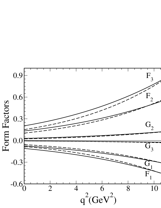
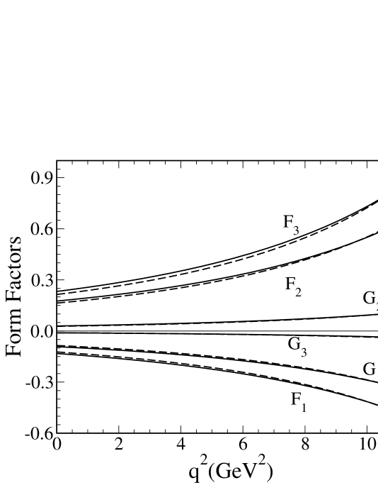
Figure 1: Form factors for $\Omega_{b}\to\Omega_{c}(1/2^{+})$ obtained using harmonic oscillator wave functions (left panel, HOSR and HONR models) and Sturmian wave functions (right panel, STSR and STSR models). In each panel, the solid curves arise from the semi-relativistic version of the model, while the dashed curves arise from the non-relativistic version.

Figure 1 shows the $q^{2}$ dependence of the form factors for the elastic transition $\Omega_{b}\to\Omega_{c}(1/2^{+})$ calculated in the HONR and HOSR models on the left, and in the STSR and STNR models on the right. In each panel, the solid curves arise from the SR version of the model, while the dashed curves are from the NR version. Here we note that the form factors calculated using the Sturmian wave functions have slopes near the non-recoil point that are similar to those calculated using the harmonic oscillator wave functions. This is due to the fact that we have similar mixing patterns for the $\Omega_{b}$ and $\Omega_{c}$ ground state wave functions in all models as can be seen in Table 5.

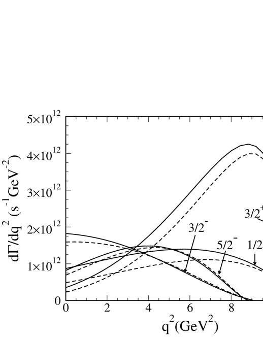
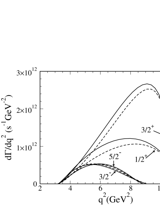
Figure 2: The differential decay rates for selected $\Omega_{b}\to\Omega_{c}^{(*)}$ transitions, in the various models that we use. The panels on the left arise from the two versions of the harmonic oscillator model, while those on the right are from the Sturmian models. The upper panels are for $\Omega_{b}\to\Omega_{c}^{(*)}\ell\bar{\nu}_{\ell}$, where $\ell$ is $e^{-}$ or $\mu^{-}$. The lower panels are for $\Omega_{b}\to\Omega_{c}^{(*)}\tau\bar{\nu}_{\tau}$. The curves are for final states with $J^{P}=3/2^{+}$, $1/2^{+}$, $3/2^{-}$ and $5/2^{-}$. In each panel, the solid curves arise from the semi-relativistic version of the model, while the dashed curves arise from the non-relativistic version.

The differential decay rates $d\Gamma/dq^{2}$ obtained in the four models for different final states in $\Omega_{b}\rightarrow\Omega_{c}^{(*)}\ell\bar{\nu}_{\ell}$, with $\ell=e^{-},\mu^{-}$, are shown in the upper panels of Figure 2. For these rates, we use $|V_{cb}|=0.041$. In these figures, we only show the differential rates for the dominant decays to the two elastic channels, with $J^{P}=3/2^{+}$ and $J^{P}=1/2^{+}$, and for two orbital excitations, the states with $J^{P}=3/2^{-}$ and $5/2^{-}$. We have also examined the differential decay rates to the $1/2^{-}$, $1/2^{-}_{1}$, and $3/2^{-}_{1}$ orbitally excited states, as well as to the radially excited states $1/2^{+}_{1}$ and $3/2^{+}_{1}$ (notations defined in Section IV.1). We have found that the branching fraction for the radially excited states (not shown in Table 8) are small, whereas the branching fraction for the decays to the orbitally excited states are not insignificant, as shown in Table 8. The lower panels of Figure 2 show the differential decay rates of $\Omega_{b}$ decaying to the same $\Omega_{c}$ final states as in the upper panels, but with a $\tau$ lepton in the final state.

In Table 8 we show the integrated decay rates obtained for the selected final states in the four quark models we use. The first part of this table shows the rate with a vanishing lepton mass, while the second part shows the rate when the final lepton is a $\tau$. The last two rows of the first part of the table present the total decay rate and the ratio of the elastic to the total semileptonic decay rate. The integrated rates for the elastic decay modes $(1/2^{+},3/2^{+})$ obtained in all models are similar. However, the two Sturmian models predict somewhat smaller rates for decays into the inelastic $\Omega_{c}$ channels. As a result the branching fraction for the elastic decay mode is smaller in the HO models than in the Sturmian models. If we consider the two HO models alone, the predicted elastic branching fraction is 49.5$\pm 1.5\%$. The corresponding prediction from the Sturmian models is 67.5$\pm 0.5\%$. Thus, the two HO models are consistent with each other, and the two ST models are consistent with each other, but the HO and ST models are in disagreement. Both sets of models predict that the elastic decay processes dominate the $\Omega_{b}$ semileptonic decay but do not saturate it; there is some significant branching fraction to the inelastic channels.

Table 8: Integrated decay rates for $\Omega_{b}\to\Omega_{c}^{(*)}$ in units of $10^{10}s^{-1}$, for a selection of $\Omega_{c}$ states in the four models we consider. The upper portion of the table presents the decay rates obtained with massless leptons (electron or muon), while the lower portion corresponds to the rates with a massive $\tau$ lepton in the final state.

	$\Omega_{b}\to\Omega^{(*)}_{c}\ell^{-}\bar{\nu}_{\ell}$
Spin	$\Gamma$(HONR)	$\Gamma$(HOSR)	$\Gamma$(STNR)	$\Gamma$(STSR)
$3/2^{+}$	$1.68$	$1.93$	2.01	2.00
$1/2^{+}$	$0.71$	$0.94$	0.87	0.96
$3/2^{-}$	$0.69$	$0.71$	0.43	0.43
$3/2^{-}_{1}$	$0.44$	$0.47$	0.23	0.22
$5/2^{-}$	$0.70$	$0.72$	0.46	0.45
$1/2^{-}$	$0.32$	$0.33$	0.20	0.20
$1/2^{-}_{1}$	$0.44$	$0.48$	0.07	0.07
total	4.98	5.58	4.27	4.33
$\Gamma_{\Omega_{c}(1/2^{+},3/2^{+})}/\Gamma_{\rm total}$	0.48	0.51	0.67	0.68
	$\Omega_{b}\to\Omega^{(*)}_{c}\tau^{-}\bar{\nu}_{\tau}$
Spin	$\Gamma$(HONR)	$\Gamma$(HOSR)	$\Gamma$(STNR)	$\Gamma$(STSR)
$3/2^{+}$	$0.81$	$0.89$	0.89	0.88
$1/2^{+}$	$0.42$	$0.49$	0.45	0.49
$3/2^{-}$	$0.15$	$0.14$	0.10	0.11
$3/2^{-}_{1}$	$0.09$	$0.10$	0.07	0.07
$5/2^{-}$	$0.14$	$0.14$	0.11	0.10
$1/2^{-}$	$0.07$	$0.06$	0.05	0.05
$1/2^{-}_{1}$	$0.08$	$0.09$	0.02	0.02
total	1.76	1.91	1.69	1.72

We may also compare our decay rates with HQET predictions. As discussed in Section III.2, there are a number of pairs of degenerate states, such as states with $J^{P}=(1/2^{+},3/2^{+})$, $J^{P}=(1/2^{-},3/2^{-})$ and $J^{P}=(3/2^{-}_{1},5/2^{-})$. In the heavy quark limit, the ratio between the rates of the ground state heavy baryon decaying to the states in the first two degenerate pairs is expected to be $1:2$, and for the third pair it is $2:3$. In other words, for example, we expect the rate for $\Omega_{b}(1/2^{+})\to\Omega_{c}(3/2^{+})$ to be twice as large as the rate for $\Omega_{b}(1/2^{+})\to\Omega_{c}(1/2^{+})$. The expected pattern of the rates coming from the HQET prediction is reflected in all of our quark model calculations, as can be seen in Table 8. Departures from these predictions are due to $1/m_{Q}$ and $1/m_{q}$ corrections, and the fact that, for instance, the $3/2^{-}$ state shown in the table is not exactly the state in the $(1/2^{-},3/2^{-})$ multiplet, but contains some admixture of the $3/2^{-}$ state from the $(3/2^{-}_{1},5/2^{-})$ multiplet.

In Table 8 we have shown only the rates to the $\Omega_{c}^{(*)}$ states which have a significant branching fraction. However, we have calculated the rates of $\Omega_{b}$ decaying to the majority of states listed in Eq. IV.1, and have found that the rates for states not shown in Table 8 are small (of the order of 1% of the total rate that we have obtained).

VI.4.2 $\Omega_{c}(\Omega_{b})\rightarrow\Xi^{(*)}$

The differential decay rates $d\Gamma/dq^{2}$ for $\Omega_{c}$ decaying to the dominant final states of $\Xi^{(*)}$ are shown as functions of $q^{2}$ in Figure 3. Here, we use $|V_{cs}|=0.224$. The left panel shows the differential decay rates obtained in the HONR and HOSR models, and the right panel shows the results from the STNR and STSR models. In both harmonic oscillator and Sturmian models we see significant differences between the non-relativistic and semi-relativistic predictions, with the most significant difference occuring between the HOSR and HONR predictions for the $1/2^{+}$ final state. Although the different size parameters obtained in various models play a role in these differences, we should also note here that this particular decay rate is very sensitive to the value of $m_{\sigma}$ ($\sigma=s$ in this decay). Our fitted values for the strange quark mass in the different models, shown in Table 1, show significant variation. We have seen similar differences between NR and SR model differential decay rates for the $\Lambda_{c}\to n$ decay mode presented in I.

Figure 3: The differential decay rates for selected $\Omega_{c}\to\Xi^{(*)}$ transitions, in the various models that we use. The panel on the left arises from the harmonic oscillator models, while the one on the right arises from the Sturmian models. They key to the curves is as in Fig. 2.

Table 9: Integrated decay rates for $\Omega_{c}\to\Xi^{(*)}$ in units of $10^{10}s^{-1}$, for selected $\Xi$ states in the four models we consider.

Spin	$\Gamma$(HONR)	$\Gamma$(HOSR)	$\Gamma$(STNR)	$\Gamma$(STSR)
$3/2^{+}$	$0.51$	$0.59$	0.36	0.39
$1/2^{+}$	$0.39$	$0.65$	0.34	0.39
$3/2^{-}$	$0.05$	$0.05$	0.03	0.02
$5/2^{-}$	$0.03$	$0.03$	0.04	0.03
$1/2^{-}$	$0.04$	$0.04$	0.05	0.05
$1/2^{-}_{1}$	$0.08$	$0.11$	0.02	0.02
total	1.10	1.47	0.84	0.90
$\Gamma_{\Xi(1/2^{+},3/2^{+})}/\Gamma_{\rm total}$	0.82	0.84	0.83	0.87

The integrated decay rates for $\Omega_{c}$ decaying to various states of $\Xi$ are shown in Table 9 in the four different models we use. The last two rows give the total decay rate and the branching fraction to the ‘elastic decay’ channels. The two elastic decay modes dominate the decay, with a small fraction of $\Omega_{c}$ decays going to the orbitally excited $\Xi^{(*)}$ states. The rates obtained in the Sturmian models are smaller than those obtained in the harmonic oscillator models. Nevertheless, the predicted elastic fraction does not depend strongly on the models we use.

Table 10: Integrated decay rates for $\Omega_{b}\to\Xi^{(*)}$ in units of $10^{12}|V_{ub}|^{2}s^{-1}$, for a selection of $\Xi$ states in the four models we consider. The last row of the top portion of the table shows the ‘elastic fraction’ (evaluated using the lowest lying $1/2^{+}$ and $3/2^{+}$ states) obtained in our model, where the decays shown in the table are assumed to saturate the semileptonic decays.

	$\Omega_{b}\to\Xi^{(*)}\ell^{-}\bar{\nu}_{\ell}$
Spin	$\Gamma$(HONR)	$\Gamma$(HOSR)	$\Gamma$(STNR)	$\Gamma$(STSR)
$3/2^{+}$	$2.90$	$3.74$	2.16	3.60
$1/2^{+}$	$0.82$	$1.46$	1.09	1.78
$3/2^{-}$	$2.17$	$2.73$	3.80	3.96
$3/2^{-}_{1}$	$2.25$	$4.15$	2.04	2.03
$5/2^{-}$	$2.15$	$3.73$	3.27	3.20
$1/2^{-}$	$0.64$	$0.87$	1.33	1.39
$1/2^{-}_{1}$	$1.15$	$1.80$	0.35	0.37
total	12.08	18.48	14.04	16.33
$\Gamma_{\Xi(1/2^{+},3/2^{+})}/\Gamma_{\rm total}$	0.31	0.28	0.23	0.33
	$\Omega_{b}\to\Xi^{(*)}\tau^{-}\bar{\nu}_{\tau}$
$3/2^{+}$	$2.42$	$3.10$	1.76	2.83
$1/2^{+}$	$0.89$	$1.53$	1.06	1.61
$3/2^{-}$	$1.86$	$2.32$	2.88	2.99
$3/2^{-}_{1}$	$1.86$	$3.36$	1.39	1.35
$5/2^{-}$	$1.62$	$2.75$	2.33	2.25
$1/2^{-}$	$0.59$	$0.77$	1.04	1.07
$1/2^{-}_{1}$	1.09	$1.67$	0.30	0.30
Total	10.33	15.50	10.76	12.4

In Table 10 the integrated decay rates of $\Omega_{b}$ to various states of $\Xi$ are presented, along with the rates for the $\Omega_{b}\to\Xi^{(*)}\tau^{-}\bar{\nu}_{\tau}$ in the second part of the table. We note that due to the large phase space available, a significant fraction of $\Omega_{b}$ is predicted to decay semileptonically to various excited $\Xi$ states. Apart from a few decay modes, such as $\Xi(1/2_{1}^{-})$, the integrated decay rates of $\Omega_{b}$ to the various states of $\Xi$ vary minimally within the models we use.

VI.4.3 $\Omega_{c}\rightarrow\Omega^{(*)}$

Table 11 shows the integrated rates for $\Omega_{c}$ decaying to $\Omega$ in our two harmonic oscillator models. The decay to the ground state ($J^{P}=3/2^{+}$) almost saturates the decay, providing 91% of the total decay rate. The lack of phase space suppresses the decays to ’inelastic’ channels.

Table 11: Integrated decay rates for $\Omega_{c}\to\Omega^{(*)}$ in units of $10^{11}s^{-1}$, for a selection of $\Omega$ states in the two HO models we consider. The last row shows the ‘elastic fraction’ obtained in our model, assuming the decays shown in the table saturate the semileptonic decays.

Spin	$\Gamma$(HONR)	$\Gamma$(HOSR)
$3/2^{+}$	$4.74$	$5.39$
$3/2^{-}$	$0.31$	$0.33$
$1/2^{-}$	$0.18$	$0.19$
total	5.23	5.91
$\Gamma_{\Omega(3/2^{+})}/\Gamma_{\rm total}$	0.91	0.91

VI.5 Form Factors and Decay Rates: $\Lambda_{Q}$, revisited

One consequence of the modified variational procedure mentioned in Section VI.1, coupled with fitting to the decay rate for $\Lambda_{c}^{+}\to\Lambda e^{+}\nu$, is that most of the decay rates for $\Lambda_{Q}$ have been modified. In this section, we briefly discuss the new results for $\Lambda_{Q}$ decays, and compare them with those presented in I. We also discuss the effects of $\kappa$ on these decay rates.

Table 12: Integrated decay rates for $\Lambda_{c}\to\Lambda^{(*)}$ in units of $10^{11}s^{-1}$, in the models we consider. The row labeled ‘total’ is obtained by adding all calculated exclusive decay rates. The fourth and fifth columns show the $\kappa$-affected integrated rates in the HO models. Integrated rates from our previous work are also shown in parentheses for comparison. The last row shows the ‘elastic fraction’ estimated in our models, assuming that the exclusive channels calculated saturate the semileptonic decays of the $\Lambda_{c}$. In each row, the numbers in parentheses are from I MWS .

$J^{P}$	$\Gamma$(HONR)	$\Gamma$(HOSR)	$\Gamma$(HONR$\kappa)$	$\Gamma$(HOSR$\kappa)$	$\Gamma$(STNR)	$\Gamma$(STSR)	Expt. CLEO
$1/2^{+}$	$1.80$ (2.10)	$2.16$ (2.36)	$1.07$	$1.31$	1.32 (0.79)	1.44 (1.11)	1.05$\pm$0.35
total	2.00 (2.36)	2.37 (2.73)	1.22	1.47	1.53 (0.97)	1.60 (1.31)	-
$\Gamma_{\Lambda}/\Gamma_{\rm total}$	0.90 (0.89)	0.91 (0.86)	0.88	0.89	0.86 (0.81)	0.90 (0.85)	1.0 (assumed)

Table 12 shows the integrated decay rates for $\Lambda_{c}\to\Lambda^{(*)}$ obtained in the various models we use. The second and third columns of this table show the rates we obtain in the two harmonic oscillator models. Note that the rates obtained in the HO models are somewhat improved from those presented in I, but are still larger than the experimentally measured rate by about a factor of two, even though the rate is included in the fit. The fourth and fifth columns show the rates we obtain when $\kappa$ is included in the harmonic oscillator form factors. The second row in the table shows the rates we obtain with the modified variational procedure, while the numbers in parentheses in that row are the corresponding rates presented in I. In the Sturmian models, the elastic rate is larger than in I, resulting in elastic fractions that are similar to those obtained in the HO models in the present work. As a result, the overall model dependence of the elastic fraction has decreased significantly. One of the reasons for this improvement is that with the new minimization scheme both harmonic oscillator and Sturmian model wave functions for different baryon states have similar mixing coefficients, as can be seen in Tables 5 and 6.

The third row presents the total rate we estimate for $\Lambda_{c}^{+}\to\Lambda^{(*)}e^{+}\nu$ (the numbers in parentheses are from I). Examination of these rates indicates that the model dependence in the $\Lambda_{c}^{+}\to\Lambda e^{+}\nu$ rate has decreased compared with I. We have obtained an average value of $1.28^{+0.16}_{-0.21}\times 10^{11}s^{-1}$ for the $\Lambda_{c}^{+}\to\Lambda e^{+}\nu$ rate in the Sturmian models and the two $\kappa$-modified HO models, consistent with the value reported by the CLEO collaboration CLEO . In the last row of Table 12 the ‘elastic fractions’ obtained in the various models are shown. Our new calculations predict smaller inelastic branching fractions (9 to 14%) than reported in I (11 to 19%). The elastic fraction, averaged over the Sturmian models and the $\kappa$-modified harmonic-oscillator models, is found to be $0.88\pm 0.02$.

Table 13: Rates for $\Lambda_{b}\to\Lambda_{c}^{(*)}$ decays in units of $10^{10}s^{-1}$. The fourth and fifth columns show the $\kappa$-affected integrated rates in the HO models. Integrated rates from our previous work are also shown in parentheses for comparison. The row labeled ‘total’ is obtained by adding all calculated exclusive decay rates, while the row with the branching fractions assumes that the exclusive channels calculated saturate the semileptonic decays of the $\Lambda_{b}$. The elastic fraction reported by the DELPHI collaboration delphi (third row of numbers, eighth column) is actually $\Gamma(\Lambda_{b}\to\Lambda_{c}\ell\bar{\nu}_{\ell})/[\Gamma(\Lambda_{b}\to\Lambda_{c}\ell\bar{\nu}_{\ell})+\Gamma(\Lambda_{b}\to\Lambda_{c}\pi\pi\ell\bar{\nu}_{\ell})]$. The errors on both numbers from DELPHI are statistical and systematic, respectively.

$J^{P}$	$\Gamma$(HONR)	$\Gamma$(HOSR)	$\Gamma$(HONR$\kappa)$	$\Gamma$(HOSR$\kappa)$	$\Gamma$(STNR)	$\Gamma$(STSR)	$\Gamma_{\rm DELPHI}$ delphi
$1/2^{+}$	$3.50$ (4.60)	$4.14$ (5.39)	$1.81$	$2.29$	2.39 (1.47)	2.52 (2.00)	$4.07^{+0.90+1.30}_{-0.65-0.98}$
Total ($\Lambda_{c}^{(*)}\ell^{-}\bar{\nu}_{\ell}$)	4.83 (5.95)	5.21 (6.82)	2.49	2.89	3.31 (2.36)	3.04 (2.88)	-
$\Gamma_{\Lambda_{c}}/\Gamma_{\rm total}$	0.72 (0.76)	0.79 (0.79)	0.73	0.79	0.72 (0.62)	0.83 (0.69)	$0.47^{+0.10+0.07}_{-0.08-0.06}$

The integrated rates for $\Lambda_{b}\to\Lambda_{c}^{(*)}$ are shown in Table 13. Here we again present both the results from this work and from I for comparison. We note that the HO and ST models now provide predictions for both the elastic ${\Lambda_{b}}\to\Lambda_{c}$ decay and the total decay rates that are more consistent with each other. It is intriguing that, for the decays of both the $\Lambda_{b}$ and $\Lambda_{c}$, the results obtained in the $\kappa$-modified HO models are consistent with the results obtained in the ST models.

The elastic fraction for the $\Lambda_{b}\to\Lambda_{c}^{(*)}$ decay obtained in the various models is shown in the last row of Table 13. In the present work this fraction is slightly less model-dependent than in I. The average value for the ${\Lambda_{b}}\to\Lambda_{c}e^{-}\nu$ rate obtained using the two Sturmian models and the two $\kappa$-modified HO models is $2.25^{+0.27}_{-0.44}\times 10^{10}s^{-1}$. These four models predict an average value of $0.77\pm 0.05$ for the elastic fraction.

Table 14: Decay rates of $\Lambda_{b}\to N^{(*)+}\ell^{-}\bar{\nu}_{\ell}$ in units of $10^{12}|V_{ub}|^{2}s^{-1}$. The fourth, fifth, eighth and ninth columns show the $\kappa$-affected integrated rates in the HO models. The row labeled ‘total’ is obtained by summing all the exclusive decay rates shown in the table. Integrated rates from our previous work are also shown in parentheses for comparison. The first four columns of numbers are for decays with a muon or electron in the final state, while the last four columns are for decays with a $\tau$ in the final state. Also shown are the rates for $\Lambda_{c}\to N^{(*)0}\ell^{+}\nu_{\ell}$ in units of $10^{10}s^{-1}$.

	$\Lambda_{b}\to N^{(*)+}\ell^{-}\bar{\nu}_{\ell}$				$\Lambda_{b}\to N^{(*)+}\tau^{-}\bar{\nu}_{\tau}$
$J^{P}$	$\Gamma$(HONR)	$\Gamma$(HOSR)	$\Gamma$(HONR$\kappa)$	$\Gamma($HOSR$\kappa)$	$\Gamma$(HONR)	$\Gamma$(HOSR)	$\Gamma$(HONR$\kappa)$	$\Gamma$(HOSR$\kappa)$
$1/2^{+}$	$2.38$ (4.55)	$3.53$ (7.55)	$0.90$	$1.19$	2.12 (4.01)	3.11 (6.55)	$0.81$	$1.06$
$1/2^{+}_{1}$	$0.44$	0.85	$0.49$	$0.65$	0.35	0.64	$0.12$	$0.22$
$1/2^{-}$	$1.18$	1.14	$0.45$	$0.42$	0.95	0.85	$0.38$	$0.35$
$3/2^{-}$	$0.87$	$0.73$	$0.20$	$0.15$	0.64	0.46	$0.17$	$0.06$
$3/2^{+}$	$0.52$	0.28	$0.11$	$0.06$	0.36	0.17	$0.09$	$0.05$
$5/2^{+}$	$1.29$	$0.44$	$0.18$	$0.06$	0.69	0.18	$0.13$	$0.04$
Total	6.68 (12.25)	6.97 (21.31)	2.33	2.53	5.11 (9.00)	5.41 (15.53)	1.70	1.78
	$\Lambda_{c}\to N^{(*)0}\ell^{+}\nu_{\ell}$				-	-	-	-
$1/2^{+}$	$0.68$	$0.84$	0.31	0.38	-	-	-	-
$1/2^{-}$	$0.03$	$0.03$	0.02	0.02	-	-	-	-

In Table 14 we present the integrated rates for $\Lambda_{b}\to N^{(*)+}\ell^{-}\bar{\nu}_{\ell}$ obtained in the two HO models. Integrated rates for $\Lambda_{b}\to N^{(*)+}\tau^{-}\bar{\nu}_{\tau}$ are also shown in this table. From the integrated rates for all allowed decay modes to ground state nucleons and N^∗ states shown in Table 14, we predict that a significant fraction of these decays are to excited nucleons, due in part to the large phase space available. We also present $\Lambda_{b}\to p$ rates and total decay rates from I in parentheses for comparison. We note that, as in the two previous decay processes, the modified variational procedure leads to results in the two HO models that are more consistent with each other.

VII Conclusion and outlook

A constituent quark model calculation of semileptonic decays of $\Omega_{Q}$, which has several intriguing features, has been described in the preceding sections. Analytic results for the form factors for the decays to ground states and excited states with a selection of quantum numbers are evaluated, and compared to HQET predictions. For $\Omega_{b}\to\Omega_{c}$ transitions, the HQET relationships among the form factors detailed in Appendix C in the $(1/2^{+},\,3/2^{+})$, $(1/2^{-},\,3/2^{-})$, $(3/2^{-},\,5/2^{-})$, and $(3/2^{+},\,5/2^{+})$ doublets are respected in our predicted form factors, at leading order.

These form factors depend on the size parameters of the initial and final baryon wave functions, and so a fit is made to the spectrum of the states treated here. Two model Hamiltonians are used, with either a nonrelativistic or semi-relativistic kinetic energy term, and with Coulomb and spin-spin contact interactions, as we did before in our work on $\Lambda_{Q}$ decay. For the present work we have modified our variational procedure from that used in I, and we have incorporated the $\Lambda_{c}^{+}\to\Lambda e^{+}\nu$ rate in the fit to the spectrum. As a result our size parameters are somewhat different from those shown in I, and our four baryon spectra are improved from those shown in I.

As in I, the wave functions are expanded in either a harmonic oscillator or Sturmian basis, up to second-order polynomials, and our numerical results for form factors and rates are calculated using the resulting mixed wave functions. Four sets of predictions are made for form factors and rates, with wave functions, size parameters and mixing coefficients arising from fits using both the non-relativistic and semi-relativistic Hamiltonians, and using the two different bases. The variation among these predictions can be used to assess the model dependence in the results we obtain.

At present there exist few quantitative measurements of the semileptonic decay rates of $\Omega_{Q}$. The CLEO collaboration cleooc has measured $B(\Omega_{c}^{0}\to\Omega^{-}e^{+}\nu)\cdot\sigma(e^{+}e^{-}\to\Omega_{c}X)=42.2\pm 14.1\pm 11.9$ fb. In addition the ARGUS argus and BELLE belle collaborations have reported the $\Omega_{c}^{0}\to\Omega^{-}$ decay as ‘seen’. However, the branching fraction for this decay has not yet been measured, which means that a comparison of our model predictions with experiment is not possible at this time. Nevertheless, it is instructive to examine our predictions for the various integrated rates for $\Omega_{b}$ and $\Omega_{c}$ decays in light of HQET predictions for these decays. There are a number of pairs of degenerate states, such as states with $J^{P}=(1/2^{+},3/2^{+})$, $J^{P}=(1/2^{-},3/2^{-})$, $J^{P}=(3/2^{-}_{1},5/2^{-})$, for which HQET predicts the relationships between the form factors as well as the ratio of rates of the degenerate pairs. According to this prediction, the rate for the $\Omega_{b}\to\Omega_{c}(3/2^{+})$ is expected to be twice as large as the rate for $\Omega_{b}\to\Omega_{c}(1/2^{+})$, and the rate for the $J^{P}=3/2^{-}$ final state is also expected to be twice as large as the rate for the $J^{P}=1/2^{-}$ final state decay. In the same way the ratio of the rates for the final states of the $(3/2^{-}_{1},\,5/2^{-})$ doublet is expected to be 2:3. The states we obtained in our spectral fits are not exactly the HQET states, but appear to be close approximations to such states, because these relationships among the rates of the degenerate pairs are well respected in all our quark model calculations for the semileptonic decays of $\Omega_{b}$.

Our predictions for the semileptonic elastic branching fraction of $\Omega_{Q}$ vary minimally within the models we use. We obtain an average value of (84$\pm$ 2%) for the elastic fraction of $\Omega_{c}\to\Xi^{(*)}$. For the case of $\Omega_{c}\to\Omega^{(*)}$, 91% of all decays are elastic. The two HO models give results that are consistent with each other (48%, 51%) for the elastic fraction of $\Omega_{b}\to\Omega_{c}^{(*)}$. The two Sturmian models also give results that are consistent with each other (67% and 68%), but which are somewhat different from the fraction predicted by the HO models.

We have recalculated the $\Lambda_{Q}$ rates in all four models. Following ISGW, we have also modified the results of the HO models by including a parameter $\kappa$ in the exponential factor that multiplies all HO form factors. As a result the model dependence of the $\Lambda_{Q}$ rates and the elastic rates have been decreased significantly. We have obtained an average value of $1.28^{+0.16}_{-0.21}\times 10^{11}s^{-1}$ for the $\Lambda_{c}^{+}\to\Lambda e^{+}\nu$ decay rate in the Sturmian and $\kappa$-modified HO models, and the elastic fraction for the decays of the $\Lambda_{c}$ is $0.88\pm 0.02$. For ${\Lambda_{b}}\to\Lambda_{c}e^{-}\nu$ our models predict an average value of $2.25^{+0.27}_{-0.44}\times 10^{10}s^{-1}$, and the predicted elastic fraction is $0.77\pm 0.05$.

As noted in I, the work presented in this manuscript can be extended in a number of directions. We can apply our model to the description of the semileptonic decays of the light baryons, although these are already successfully described by Cabibbo theory. Essentially all experimentally accessible observables for these decays have been measured, and it will be interesting to see if our model, constructed with no special reference to chiral symmetry or current algebra, can describe the results of these measurements.

We have not examined the predictions of our model for the many polarization observables which can, in principle, be measured in semileptonic decays. In addition, the rare decays of heavy baryons, such as $\Omega_{b}\to\Omega$ can easily be treated in the framework that we have developed. Such processes, along with their meson analogs, are used in searches for physics beyond the Standard Model. However, the interpretation of the measured rates depend strongly on estimates of the form factors involved (in much the same way that extraction of CKM matrix elements depends on the form factors that describe semileptonic decays). Finally, if factorization in some form is valid, the semileptonic form factors calculated in the manuscript may also be useful in the description of nonleptonic weak decays.

It may also be possible to systematically improve the quark model used in the present calculation. An obvious first step is the implementation of full symmetrization of the spatial wave functions in the Sturmian basis, which would allow calculation of results for decays to final state nucleons in this basis.

We also plan to modify and expand all our baryon spectrum codes to make predictions for baryons containing quarks with three different masses. One advantage of this modification is that it will allow us to examine the semileptonic decays of $\Xi_{Q}$. This study will be interesting, as some of the $\Xi_{Q}$ states have an antisymmetric ($\Lambda_{Q}$-like) light diquark, while some have a symmetric ($\Omega_{Q}$-like) light diquark pdgxi .

Appendix A Wave Functions

The wave function components for states that we consider are shown here. These components are valid for both the $\Omega_{Q}$ and $\Xi$ states that are treated in this manuscript. For $J^{P}=1/2^{+}$, wave functions are expanded as

$$\Psi^{\Omega_{Q}}_{1/2^{+}M} = \phi_{\Omega_{Q}}\left(\vphantom{\sum_{i}}\left[\eta_{1}^{\Omega_{Q}}\psi_{000000}({\bf p}_{\rho},{\bf p}_{\lambda})+\eta_{2}^{\Omega_{Q}}\psi_{001000}({\bf p}_{\rho},{\bf p}_{\lambda})+\eta_{3}^{\Omega_{Q}}\psi_{000010}({\bf p}_{\rho},{\bf p}_{\lambda})\right]\chi_{1/2}^{\lambda}(M)\right.$$ (65)

$$+ \eta_{4}^{\Omega_{Q}}\psi_{000101}({\bf p}_{\rho},{\bf p}_{\lambda})\chi_{1/2}^{\rho}(M)+\eta_{5}^{\Omega_{Q}}\left[\psi_{1M_{L}0101}({\bf p}_{\rho},{\bf p}_{\lambda})\chi_{1/2}^{\rho}(M-M_{L})\right]^{1/2}_{M}$$

$$+ \eta_{6}^{\Omega_{Q}}\left[\psi_{2M_{L}0200}({\bf p}_{\rho},{\bf p}_{\lambda})\chi_{3/2}^{S}(M-M_{L})\right]^{1/2}_{M}$$

$$+ \left.\eta_{7}^{\Omega_{Q}}\left[\psi_{2M_{L}0002}({\bf p}_{\rho},{\bf p}_{\lambda})\chi_{3/2}^{S}(M-M_{L})\right]^{1/2}_{M}\right),$$

For $\Omega_{Q}$ states with $J^{P}=3/2^{+}$, the expansion is

$$\Psi^{\Omega_{Q}}_{3/2^{+}M} = \phi_{\Omega_{Q}}\left(\vphantom{\sum_{i}}\left[\eta_{1}^{\Omega_{Q}}\psi_{000000}({\bf p}_{\rho},{\bf p}_{\lambda})+\eta_{2}^{\Omega_{Q}}\psi_{001000}({\bf p}_{\rho},{\bf p}_{\lambda})+\eta_{3}^{\Omega_{Q}}\psi_{000010}({\bf p}_{\rho},{\bf p}_{\lambda})\right]\chi_{3/2}^{S}(M)\right.$$ (66)

$$+ \eta_{4}^{\Omega_{Q}}\left[\psi_{1M_{L}0101}({\bf p}_{\rho},{\bf p}_{\lambda})\chi_{1/2}^{\rho}(M-M_{L})\right]^{3/2}_{M}$$

$$+ \eta_{5}^{\Omega_{Q}}\left[\psi_{2M_{L}0200}({\bf p}_{\rho},{\bf p}_{\lambda})\chi_{3/2}^{S}(M-M_{L})\right]^{3/2}_{M}$$

$$+ \eta_{6}^{\Omega_{Q}}\left[\psi_{2M_{L}0200}({\bf p}_{\rho},{\bf p}_{\lambda})\chi_{1/2}^{\lambda}(M-M_{L})\right]^{3/2}_{M}$$

$$+ \eta_{7}^{\Omega_{Q}}\left[\psi_{2M_{L}0101}({\bf p}_{\rho},{\bf p}_{\lambda})\chi_{1/2}^{\rho}(M-M_{L})\right]^{3/2}_{M}$$

$$+ \eta_{8}^{\Omega_{Q}}\left[\psi_{2M_{L}0002}({\bf p}_{\rho},{\bf p}_{\lambda})\chi_{3/2}^{S}(M-M_{L})\right]^{3/2}_{M}$$

$$+ \left.\eta_{9}^{\Omega_{Q}}\left[\psi_{2M_{L}0002}({\bf p}_{\rho},{\bf p}_{\lambda})\chi_{1/2}^{\lambda}(M-M_{L})\right]^{3/2}_{M}\right),$$

where $\left[\psi_{LM_{L}n_{\rho}\ell_{\rho}n_{\lambda}\ell_{\lambda}}({\bf p}_{\rho},{\bf p}_{\lambda})\chi_{S}(M-M_{L})\right]^{J}_{M}$ is a shorthand notation that denotes the Clebsch-Gordan sum $\sum_{M_{L}}\langle JM|LM_{L},SM-M_{L}\rangle\psi_{LM_{L}n_{\rho}\ell_{\rho}n_{\lambda}\ell_{\lambda}}({\bf p}_{\rho},{\bf p}_{\lambda})\chi_{S}(M-M_{L})$.

For $J^{P}=1/2^{-}$ and $3/2^{-}$, the expansion is

$$\Psi^{\Omega_{Q}}_{J^{-}M} = \phi_{\Omega_{Q}}\left(\eta_{1}^{\Omega_{Q}}\left[\psi_{1M_{L}0100}({\bf p}_{\rho},{\bf p}_{\lambda})\chi_{1/2}^{\rho}(M-M_{L})\right]^{J}_{M}\right.$$ (67)

$$+\eta_{2}^{\Omega_{Q}}\left[\psi_{1M_{L}0001}({\bf p}_{\rho},{\bf p}_{\lambda})\chi_{3/2}^{S}(M-M_{L})\right]^{J}_{M}$$

$$+\left.\eta_{3}^{\Omega_{Q}}\left[\psi_{1M_{L}0001}({\bf p}_{\rho},{\bf p}_{\lambda})\chi_{1/2}^{\lambda}(M-M_{L})\right]^{J}_{M}\right),$$

where $J$ can take the values 1/2 or 3/2.

For $J^{P}=5/2^{+}$, the expansion is

$$\Psi^{\Omega_{Q}}_{5/2^{+}M} = \phi_{\Omega_{Q}}\left(\vphantom{\sum_{i}}\eta_{1}^{\Omega_{Q}}\psi_{2M_{L}0101}({\bf p}_{\rho},{\bf p}_{\lambda})\chi_{1/2}^{\rho}(M-M_{L})+\eta_{2}^{\Omega_{Q}}\left[\psi_{2M_{L}0200}({\bf p}_{\rho},{\bf p}_{\lambda})\chi_{3/2}^{S}(M-M_{L})\right]^{5/2}_{M}\right.$$ (68)

$$+ \eta_{3}^{\Omega_{Q}}\left[\psi_{2M_{L}0200}({\bf p}_{\rho},{\bf p}_{\lambda})\chi_{1/2}^{\lambda}(M-M_{L})\right]^{5/2}_{M}+\eta_{4}^{\Omega_{Q}}\left[\psi_{2M_{L}0002}({\bf p}_{\rho},{\bf p}_{\lambda})\chi_{3/2}^{S}(M-M_{L})\right]^{5/2}_{M}$$

$$+ \left.\eta_{5}^{\Omega_{Q}}\left[\psi_{2M_{L}0002}({\bf p}_{\rho},{\bf p}_{\lambda})\chi_{1/2}^{\lambda}(M-M_{L})\right]^{5/2}_{M}\right)$$

For $J^{P}=5/2^{-}$, the wave function is

$$\Psi^{\Omega_{Q}}_{J^{-}M}=\phi_{\Omega_{Q}}\left[\psi_{1M_{L}0001}({\bf p}_{\rho},{\bf p}_{\lambda})\chi_{3/2}^{S}(M-M_{L})\right]^{5/2}_{M},$$ (69)

No other states are expected to have significant overlap with the decaying ground-state $\Omega_{Q}$ in the spectator approximation that we use.

Appendix B Quark Model Form Factors

In this section, we present the analytic expressions we obtained for the form factors, assuming single component wave functions. We list both harmonic oscillator and Sturmian form factors together, ordered by the spin and parity of the daughter baryon, beginning with the ground state. We place the form factors for each spin and parity in a separate subsection.

For most of the $J^{P}$ we treat, there is usually more than one example of the state: the exception is $5/2^{-}$, for which there is a single state up to $N=2$. We therefore distinguish among the different states with the same $J^{P}$ by presenting their quark model quantum numbers, in the notation $|n_{S},L,n_{\rho},\ell_{\rho},n_{\lambda},\ell_{\lambda}>$. Here $n_{S}$ takes values between 1 and 3, with 1 denoting total quark spin 1/2, with spin wave function of type $\chi_{\rho}$, 2 denoting total quark spin 1/2, with spin wave function of type $\chi_{\lambda}$, and 3 denoting total quark spin 3/2.

B.1 $1/2^{+},|200000>$

B.1.1 Harmonic Oscillator Form Factors

$$F_{1} = -I_{H}\left[1+\frac{m_{\sigma}}{\alpha^{2}_{\lambda\lambda^{\prime}}}\left(\frac{\alpha^{2}_{\lambda^{\prime}}}{m_{q}}+\frac{\alpha^{2}_{\lambda}}{m_{Q}}\right)\right],$$

$$F_{2} = 2I_{H}\left[1-\frac{m_{\sigma}}{\alpha^{2}_{\lambda\lambda^{\prime}}}\left(\frac{\alpha^{2}_{\lambda^{\prime}}}{2m_{q}}-\frac{\alpha^{2}_{\lambda}}{m_{Q}}\right)\right],$$

$$F_{3} = 2I_{H}\left[1+\frac{m_{\sigma}}{\alpha^{2}_{\lambda\lambda^{\prime}}}\left(\frac{\alpha^{2}_{\lambda^{\prime}}}{m_{q}}-\frac{\alpha^{2}_{\lambda}}{2m_{Q}}\right)\right],$$

$$G_{1} = -I_{H},$$

$$G_{2} = I_{H}\frac{m_{\sigma}}{m_{q}}\frac{\alpha^{2}_{\lambda^{\prime}}}{\alpha^{2}_{\lambda\lambda^{\prime}}},$$

$$G_{3} = -I_{H}\frac{m_{\sigma}}{m_{Q}}\frac{\alpha^{2}_{\lambda}}{\alpha^{2}_{\lambda\lambda^{\prime}}},$$

where

$$I_{H}=\frac{1}{3}\left(\frac{\alpha_{\lambda}\alpha_{\lambda^{\prime}}}{\alpha_{\lambda\lambda^{\prime}}^{2}}\right)^{3/2}\exp\left(-\frac{3m^{2}_{\sigma}}{2m^{2}_{\Omega_{q}}}\frac{p^{2}}{\alpha_{\lambda\lambda^{\prime}}^{2}}\right).$$

$\alpha_{\lambda\lambda^{\prime}}^{2}=\frac{1}{2}(\alpha_{\lambda}^{2}+\alpha_{\lambda^{\prime}}^{2})$, and $m_{\sigma}$ is the mass of the light quark.

B.1.2 Sturmian Form Factors

$$F_{1} = -I_{S}\left[1+\frac{m_{\sigma}}{\beta_{\lambda\lambda^{\prime}}}\left(\frac{\beta_{\lambda^{\prime}}}{m_{q}}+\frac{\beta_{\lambda}}{m_{Q}}\right)\right],$$

$$F_{2} = 2I_{S}\left[1-\frac{m_{\sigma}}{\beta_{\lambda\lambda^{\prime}}}\left(\frac{\beta_{\lambda^{\prime}}}{2m_{q}}-\frac{\beta_{\lambda}}{m_{Q}}\right)\right],$$

$$F_{3} = 2I_{S}\left[1+\frac{m_{\sigma}}{\beta_{\lambda\lambda^{\prime}}}\left(\frac{\beta_{\lambda^{\prime}}}{m_{q}}-\frac{\beta_{\lambda}}{2m_{Q}}\right)\right],$$

$$G_{1} = -I_{S},$$

$$G_{2} = I_{S}\frac{m_{\sigma}\beta_{\lambda^{\prime}}}{m_{q}\beta_{\lambda\lambda^{\prime}}},$$

$$G_{3} = -I_{S}\frac{m_{\sigma}\beta_{\lambda}}{m_{Q}\beta_{\lambda\lambda^{\prime}}},$$

where

$$I_{S}=\frac{1}{3}\frac{\left(\frac{\beta_{\lambda}\beta_{\lambda^{\prime}}}{\beta_{\lambda\lambda^{\prime}}^{2}}\right)^{3/2}}{\left[1+\frac{3}{2}\frac{m^{2}_{\sigma}}{m^{2}_{\Omega_{q}}}\frac{p^{2}}{\beta_{\lambda\lambda^{\prime}}^{2}}\right]^{2}},$$

and $\beta_{\lambda\lambda^{\prime}}=\frac{1}{2}(\beta_{\lambda}+\beta_{\lambda}^{\prime})$.

B.2 $1/2^{+}_{1},|200010>$

B.2.1 Harmonic Oscillator Form Factors

$$F_{1} = -I_{H}\frac{1}{2\alpha_{\lambda}\alpha_{\lambda^{\prime}}}\left[\left(\alpha^{2}_{\lambda}-\alpha^{2}_{\lambda^{\prime}}\right)+\frac{m_{\sigma}}{3\alpha^{2}_{\lambda\lambda^{\prime}}}\left(\frac{\alpha^{2}_{\lambda^{\prime}}(7\alpha^{2}_{\lambda}-3\alpha^{2}_{\lambda^{\prime}})}{m_{q}}+\frac{\alpha^{2}_{\lambda}(3\alpha^{2}_{\lambda}-7\alpha^{2}_{\lambda^{\prime}})}{m_{Q}}\right)\right],$$

$$F_{2} = I_{H}\frac{1}{\alpha_{\lambda}\alpha_{\lambda^{\prime}}}\left[\left(\alpha^{2}_{\lambda}-\alpha^{2}_{\lambda^{\prime}}\right)-\frac{m_{\sigma}}{3\alpha^{2}_{\lambda\lambda^{\prime}}}\left(\frac{\alpha^{2}_{\lambda^{\prime}}(7\alpha^{2}_{\lambda}-3\alpha^{2}_{\lambda^{\prime}})}{2m_{q}}-\frac{\alpha^{2}_{\lambda}(3\alpha^{2}_{\lambda}-7\alpha^{2}_{\lambda^{\prime}})}{m_{Q}}\right)\right],$$

$$F_{3} = I_{H}\frac{1}{\alpha_{\lambda}\alpha_{\lambda^{\prime}}}\left[\left(\alpha^{2}_{\lambda}-\alpha^{2}_{\lambda^{\prime}}\right)+\frac{m_{\sigma}}{3\alpha^{2}_{\lambda\lambda^{\prime}}}\left(\frac{\alpha^{2}_{\lambda^{\prime}}(7\alpha^{2}_{\lambda}-3\alpha^{2}_{\lambda^{\prime}})}{m_{q}}-\frac{\alpha^{2}_{\lambda}(3\alpha^{2}_{\lambda}-7\alpha^{2}_{\lambda^{\prime}})}{2m_{Q}}\right)\right],$$

$$G_{1} = -I_{H}\frac{\left(\alpha^{2}_{\lambda}-\alpha^{2}_{\lambda^{\prime}}\right)}{2\alpha_{\lambda}\alpha_{\lambda^{\prime}}},$$

$$G_{2} = I_{H}\frac{m_{\sigma}}{6m_{q}}\frac{\alpha_{\lambda^{\prime}}(7\alpha^{2}_{\lambda}-3\alpha^{2}_{\lambda^{\prime}})}{\alpha_{\lambda}\alpha^{2}_{\lambda\lambda^{\prime}}},$$

$$G_{3} = -I_{H}\frac{m_{\sigma}}{6m_{Q}}\frac{\alpha_{\lambda}(3\alpha^{2}_{\lambda}-7\alpha^{2}_{\lambda^{\prime}})}{\alpha_{\lambda^{\prime}}\alpha^{2}_{\lambda\lambda^{\prime}}},$$

where

$$I_{H}=\frac{1}{\sqrt{6}}\left(\frac{\alpha_{\lambda}\alpha_{\lambda^{\prime}}}{\alpha_{\lambda\lambda^{\prime}}^{2}}\right)^{5/2}\exp\left(-\frac{3m^{2}_{\sigma}}{2m^{2}_{\Omega_{q}}}\frac{p^{2}}{\alpha_{\lambda\lambda^{\prime}}^{2}}\right).$$

B.2.2 Sturmian Form Factors

$$F_{1} = -I_{S}\frac{1}{2\beta_{\lambda}\beta_{\lambda^{\prime}}}\left[(\beta^{2}_{\lambda}-\beta^{2}_{\lambda^{\prime}})+\frac{2m_{\sigma}}{3}\left(\frac{\beta_{\lambda^{\prime}}(5\beta_{\lambda}-3\beta_{\lambda^{\prime}})}{m_{q}}+\frac{\beta_{\lambda}(3\beta_{\lambda}-5\beta_{\lambda^{\prime}})}{m_{Q}}\right)\right],$$

$$F_{2} = I_{S}\frac{1}{\beta_{\lambda}\beta_{\lambda^{\prime}}}\left[(\beta^{2}_{\lambda}-\beta^{2}_{\lambda^{\prime}})-\frac{2m_{\sigma}}{3}\left(\frac{\beta_{\lambda^{\prime}}(5\beta_{\lambda}-3\beta_{\lambda^{\prime}})}{2m_{q}}-\frac{\beta_{\lambda}(3\beta_{\lambda}-5\beta_{\lambda^{\prime}})}{m_{Q}}\right)\right],$$

$$F_{3} = I_{S}\frac{1}{\beta_{\lambda}\beta_{\lambda^{\prime}}}\left[(\beta^{2}_{\lambda}-\beta^{2}_{\lambda^{\prime}})+\frac{2m_{\sigma}}{3}\left(\frac{\beta_{\lambda^{\prime}}(5\beta_{\lambda}-3\beta_{\lambda^{\prime}})}{m_{q}}-\frac{\beta_{\lambda}(3\beta_{\lambda}-5\beta_{\lambda^{\prime}})}{2m_{Q}}\right)\right],$$

$$G_{1} = -I_{S}\frac{(\beta^{2}_{\lambda}-\beta^{2}_{\lambda^{\prime}})}{2\beta_{\lambda}\beta_{\lambda^{\prime}}},$$

$$G_{2} = I_{S}\frac{m_{\sigma}}{3m_{q}}\frac{(5\beta_{\lambda}-3\beta_{\lambda^{\prime}})}{\beta_{\lambda}},$$

$$G_{3} = -I_{S}\frac{m_{\sigma}}{3m_{Q}}\frac{(3\beta_{\lambda}-5\beta_{\lambda^{\prime}})}{\beta_{\lambda^{\prime}}},$$

where

$$I_{S}=\frac{1}{2\sqrt{3}}\frac{\left(\frac{\beta_{\lambda}\beta_{\lambda^{\prime}}}{\beta_{\lambda\lambda^{\prime}}^{2}}\right)^{5/2}}{\left[1+\frac{3}{2}\frac{m^{2}_{\sigma}}{m^{2}_{\Omega_{q}}}\frac{p^{2}}{\beta_{\lambda\lambda^{\prime}}^{2}}\right]^{3}}.$$

B.3 $1/2^{+}_{2},|320002>$

B.3.1 Harmonic Oscillator Form Factors

$$F_{1} = -I_{H}m_{\sigma}\left(\frac{1}{m_{q}}-\frac{1}{m_{Q}}\right),$$

$$F_{2} = I_{H}\frac{m_{\sigma}}{2}\left(\frac{1}{m_{q}}-\frac{1}{m_{Q}}\right),$$

$$F_{3} = I_{H}\frac{m_{\sigma}}{2}\left(\frac{1}{m_{q}}-\frac{1}{m_{Q}}\right),$$

$$G_{1} = 0,$$

$$G_{2} = I_{H}\frac{m_{\sigma}}{\alpha_{\lambda}}\left[\frac{18m_{\sigma}}{5\alpha_{\lambda}}-\frac{\alpha_{\lambda}}{2}\left(\frac{4}{m_{q}}+\frac{3}{m_{Q}}\right)\right],$$

$$G_{3} = -I_{H}\frac{m_{\sigma}}{\alpha_{\lambda}}\left(\frac{18m_{\sigma}}{5\alpha_{\lambda}}+\frac{\alpha_{\lambda}}{2m_{Q}}\right),$$

where

$$I_{H}=-\frac{\sqrt{10}}{3\sqrt{3}}\left(\frac{\alpha_{\lambda}\alpha_{\lambda^{\prime}}}{\alpha_{\lambda\lambda^{\prime}}^{2}}\right)^{7/2}\exp\left(-\frac{3m^{2}_{\sigma}}{2m^{2}_{\Omega_{q}}}\frac{p^{2}}{\alpha_{\lambda\lambda^{\prime}}^{2}}\right).$$

B.3.2 Sturmian Form Factors

$$F_{1} = -I_{S}\frac{m_{\sigma}\beta_{\lambda\lambda^{\prime}}}{2\beta_{\lambda}}\left(\frac{1}{m_{q}}-\frac{1}{m_{Q}}\right),$$

$$F_{2} = I_{S}\frac{m_{\sigma}\beta_{\lambda\lambda^{\prime}}}{4\beta_{\lambda}}\left(\frac{1}{m_{q}}-\frac{1}{m_{Q}}\right),$$

$$F_{3} = I_{S}\frac{m_{\sigma}\beta_{\lambda\lambda^{\prime}}}{4\beta_{\lambda}}\left(\frac{1}{m_{q}}-\frac{1}{m_{Q}}\right),$$

$$G_{1} = 0,$$

$$G_{2} = I_{S}\frac{m_{\sigma}}{\beta_{\lambda}}\left[\frac{27m_{\sigma}}{5\beta_{\lambda}}-\frac{\beta_{\lambda\lambda^{\prime}}}{4}\left(\frac{4}{m_{q}}+\frac{3}{m_{Q}}\right)\right],$$

$$G_{3} = -I_{S}\frac{m_{\sigma}}{\beta_{\lambda}}\left(\frac{27m_{\sigma}}{5\beta_{\lambda}}+\frac{\beta_{\lambda\lambda^{\prime}}}{4m_{Q}}\right),$$

where

$$I_{S}=-\frac{4\sqrt{5}}{9}\frac{\left(\frac{\beta_{\lambda}\beta_{\lambda^{\prime}}}{\beta_{\lambda\lambda^{\prime}}^{2}}\right)^{7/2}}{\left[1+\frac{3}{2}\frac{m^{2}_{\sigma}}{m^{2}_{\Omega_{q}}}\frac{p^{2}}{\beta_{\lambda\lambda^{\prime}}^{2}}\right]^{4}}.$$

B.4 $1/2^{-},|210001>$

B.4.1 Harmonic Oscillator Form Factors

$$F_{1} = -I_{H}\frac{\alpha_{\lambda}}{6}\left(\frac{1}{m_{q}}+\frac{5}{m_{Q}}\right),$$

$$F_{2} = I_{H}\left\{\frac{2m_{\sigma}}{\alpha_{\lambda}}\left[1-\frac{m_{\sigma}}{\alpha_{\lambda\lambda^{\prime}}^{2}}\left(\frac{2\alpha_{\lambda^{\prime}}^{2}}{m_{q}}-\frac{\alpha_{\lambda}^{2}}{m_{Q}}\right)\right]-\frac{\alpha_{\lambda}}{6m_{q}}\right\},$$

$$F_{3} = I_{H}\frac{4m_{\sigma}}{\alpha_{\lambda}}\left[1+\frac{m_{\sigma}}{\alpha_{\lambda\lambda^{\prime}}^{2}}\left(\frac{\alpha^{2}_{\lambda^{\prime}}}{m_{q}}-\frac{\alpha^{2}_{\lambda}}{2m_{Q}}\right)\right],$$

$$G_{1} = I_{H}\left(\frac{2m_{\sigma}}{\alpha_{\lambda}}-\frac{5\alpha_{\lambda}}{6m_{Q}}\right),$$

$$G_{2} = -I_{H}\left[\frac{2m_{\sigma}}{\alpha_{\lambda}}-\alpha_{\lambda}\left(\frac{1}{2m_{q}}+\frac{2}{3m_{Q}}\right)\right],$$

$$G_{3} = I_{H}\frac{2\alpha_{\lambda}}{3m_{Q}},$$

where

$$I_{H}=-\frac{1}{3}\left(\frac{\alpha_{\lambda}\alpha_{\lambda^{\prime}}}{\alpha_{\lambda\lambda^{\prime}}^{2}}\right)^{5/2}\exp\left(-\frac{3m^{2}_{\sigma}}{2m^{2}_{\Omega_{q}}}\frac{p^{2}}{\alpha_{\lambda\lambda^{\prime}}^{2}}\right).$$

B.4.2 Sturmian Form Factors

$$F_{1} = -I_{S}\frac{\beta_{\lambda\lambda^{\prime}}}{12}\left(\frac{1}{m_{q}}+\frac{5}{m_{Q}}\right),$$

$$F_{2} = I_{S}\left\{\frac{2m_{\sigma}}{\beta_{\lambda}}\left[1-\frac{m_{\sigma}}{\beta_{\lambda\lambda^{\prime}}}\left(\frac{2\beta_{\lambda^{\prime}}}{m_{q}}-\frac{\beta_{\lambda}}{m_{Q}}\right)\right]-\frac{\beta_{\lambda\lambda^{\prime}}}{12m_{q}}\right\},$$

$$F_{3} = I_{S}\frac{4m_{\sigma}}{\beta_{\lambda}}\left[1+\frac{m_{\sigma}}{\beta_{\lambda\lambda^{\prime}}}\left(\frac{\beta_{\lambda^{\prime}}}{m_{q}}-\frac{\beta_{\lambda}}{2m_{Q}}\right)\right],$$

$$G_{1} = I_{S}\left(\frac{2m_{\sigma}}{\beta_{\lambda}}-\frac{5\beta_{\lambda\lambda^{\prime}}}{12m_{Q}}\right),$$

$$G_{2} = -I_{S}\left[\frac{2m_{\sigma}}{\beta_{\lambda}}-\beta_{\lambda\lambda^{\prime}}\left(\frac{1}{4m_{q}}+\frac{1}{3m_{Q}}\right)\right],$$

$$G_{3} = I_{S}\frac{\beta_{\lambda\lambda^{\prime}}}{3m_{Q}},$$

where

$$I_{S}=-\frac{\sqrt{2}}{3}\frac{\left(\frac{\beta_{\lambda}\beta_{\lambda^{\prime}}}{\beta_{\lambda\lambda^{\prime}}^{2}}\right)^{5/2}}{\left[1+\frac{3}{2}\frac{m^{2}_{\sigma}}{m^{2}_{\Omega_{q}}}\frac{p^{2}}{\beta_{\lambda\lambda^{\prime}}^{2}}\right]^{3}}.$$

B.5 $3/2^{-},|210001>$

B.5.1 Harmonic Oscillator Form Factors

$$F_{1} = -I_{H}\frac{m_{\sigma}}{\alpha_{\lambda}}\left[1+\frac{m_{\sigma}}{\alpha^{2}_{\lambda\lambda^{\prime}}}\left(\frac{\alpha^{2}_{\lambda^{\prime}}}{m_{q}}+\frac{\alpha^{2}_{\lambda}}{m_{Q}}\right)\right],$$

$$F_{2} = I_{H}\left\{\frac{2m_{\sigma}}{\alpha_{\lambda}}\left[1-\frac{m_{\sigma}}{2\alpha_{\lambda\lambda^{\prime}}^{2}}\left(\frac{\alpha_{\lambda^{\prime}}^{2}}{m_{q}}-\frac{2\alpha_{\lambda}^{2}}{m_{Q}}\right)\right]-\frac{\alpha_{\lambda}}{3m_{q}}\right\},$$

$$F_{3} = I_{H}\left\{\frac{2m_{\sigma}}{\alpha_{\lambda}}\left[1+\frac{m_{\sigma}}{2\alpha_{\lambda\lambda^{\prime}}^{2}}\left(\frac{2\alpha^{2}_{\lambda^{\prime}}}{m_{q}}-\frac{\alpha^{2}_{\lambda}}{m_{Q}}\right)\right]-\frac{\alpha_{\lambda}}{6}\left(\frac{2}{m_{q}}+\frac{1}{m_{Q}}\right)\right\},$$

$$F_{4} = I_{H}\frac{\alpha_{\lambda}}{3}\left(\frac{2}{m_{q}}+\frac{1}{m_{Q}}\right),$$

$$G_{1} = -I_{H}\left(\frac{m_{\sigma}}{\alpha_{\lambda}}+\frac{\alpha_{\lambda}}{6m_{Q}}\right),$$

$$G_{2} = I_{H}\frac{m_{\sigma}^{2}}{m_{q}}\frac{\alpha^{2}_{\lambda^{\prime}}}{\alpha^{2}_{\lambda\lambda^{\prime}}\alpha_{\lambda}},$$

$$G_{3} = -I_{H}\frac{\alpha_{\lambda}}{m_{Q}}\left(\frac{m_{\sigma}^{2}}{\alpha^{2}_{\lambda\lambda^{\prime}}}-\frac{1}{6}\right),\,\,\,\,\,\,\,\,\,\,\,\,\,\,G_{4}=-I_{H}\frac{\alpha_{\lambda}}{3m_{Q}},$$

$$I_{H} = -\frac{1}{\sqrt{3}}\left(\frac{\alpha_{\lambda}\alpha_{\lambda^{\prime}}}{\alpha_{\lambda\lambda^{\prime}}^{2}}\right)^{5/2}\exp\left(-\frac{3m^{2}_{\sigma}}{2m^{2}_{\Omega_{q}}}\frac{p^{2}}{\alpha_{\lambda\lambda^{\prime}}^{2}}\right).$$

B.5.2 Sturmian Form Factors

$$F_{1} = -I_{S}\frac{m_{\sigma}}{\beta_{\lambda}}\left[1+\frac{m_{\sigma}}{\beta_{\lambda\lambda^{\prime}}}\left(\frac{\beta_{\lambda^{\prime}}}{m_{q}}+\frac{\beta_{\lambda}}{m_{Q}}\right)\right],$$

$$F_{2} = I_{S}\left\{\frac{2m_{\sigma}}{\beta_{\lambda}}\left[1-\frac{m_{\sigma}}{\beta_{\lambda\lambda^{\prime}}}\left(\frac{\beta_{\lambda^{\prime}}}{2m_{q}}-\frac{\beta_{\lambda}}{m_{Q}}\right)\right]-\frac{\beta_{\lambda\lambda^{\prime}}}{6m_{q}}\right\},$$

$$F_{3} = I_{S}\left\{\frac{2m_{\sigma}}{\beta_{\lambda}}\left[1+\frac{m_{\sigma}}{\beta_{\lambda\lambda^{\prime}}}\left(\frac{\beta_{\lambda^{\prime}}}{m_{q}}-\frac{\beta_{\lambda}}{2m_{Q}}\right)\right]-\frac{\beta_{\lambda\lambda^{\prime}}}{12}\left(\frac{2}{m_{q}}+\frac{1}{m_{Q}}\right)\right\},$$

$$F_{4} = I_{S}\frac{\beta_{\lambda\lambda^{\prime}}}{6}\left(\frac{2}{m_{q}}+\frac{1}{m_{Q}}\right),$$

$$G_{1} = -I_{S}\left(\frac{m_{\sigma}}{\beta_{\lambda}}+\frac{\beta_{\lambda\lambda^{\prime}}}{12m_{Q}}\right),$$

$$G_{2} = I_{S}\frac{m^{2}_{\sigma}}{m_{q}}\frac{\beta_{\lambda^{\prime}}}{\beta_{\lambda}\beta_{\lambda\lambda^{\prime}}},$$

$$G_{3} = -I_{S}\frac{\beta_{\lambda\lambda^{\prime}}}{m_{Q}}\left(\frac{m^{2}_{\sigma}}{\beta_{\lambda\lambda^{\prime}}^{2}}-\frac{1}{12}\right),\,\,\,\,\,\,\,\,\,\,\,\,\,\,G_{4}=-I_{S}\frac{\beta_{\lambda\lambda^{\prime}}}{6m_{Q}},$$

$$I_{S} = -\sqrt{\frac{2}{3}}\frac{\left(\frac{\beta_{\lambda}\beta_{\lambda^{\prime}}}{\beta_{\lambda\lambda^{\prime}}^{2}}\right)^{5/2}}{\left[1+\frac{3}{2}\frac{m^{2}_{\sigma}}{m^{2}_{\Omega_{q}}}\frac{p^{2}}{\beta_{\lambda\lambda^{\prime}}^{2}}\right]^{3}}.$$

B.6 $1/2^{-}_{1},|310001>$

B.6.1 Harmonic Oscillator Form Factors

$$F_{1} = -I_{H}\frac{\alpha_{\lambda}}{3}\left(\frac{1}{m_{q}}-\frac{1}{m_{Q}}\right),$$

$$F_{2} = I_{H}\left\{\frac{m_{\sigma}}{\alpha_{\lambda}}\left[1+\frac{m_{\sigma}}{\alpha_{\lambda\lambda^{\prime}}^{2}}\left(\frac{\alpha^{2}_{\lambda^{\prime}}}{m_{q}}+\frac{\alpha^{2}_{\lambda}}{m_{Q}}\right)\right]-\frac{\alpha_{\lambda}}{3m_{Q}}\right\},$$

$$F_{3} = -I_{H}\frac{m_{\sigma}}{\alpha_{\lambda}}\left[1+\frac{m_{\sigma}}{\alpha_{\lambda\lambda^{\prime}}^{2}}\left(\frac{\alpha^{2}_{\lambda^{\prime}}}{m_{q}}+\frac{\alpha^{2}_{\lambda}}{m_{Q}}\right)\right],$$

$$G_{1} = -I_{H}\left(\frac{2m_{\sigma}}{\alpha_{\lambda}}-\frac{\alpha_{\lambda}}{3m_{Q}}\right),$$

$$G_{2} = -I_{H}\left[\frac{m_{\sigma}}{\alpha_{\lambda}}-\frac{\alpha_{\lambda}}{3}\left(\frac{3}{m_{q}}+\frac{1}{m_{Q}}\right)\right],$$

$$G_{3} = I_{H}\left(\frac{3m_{\sigma}}{\alpha_{\lambda}}+\frac{\alpha_{\lambda}}{3m_{Q}}\right),$$

where

$$I_{H}=-\frac{\sqrt{2}}{3}\left(\frac{\alpha_{\lambda}\alpha_{\lambda^{\prime}}}{\alpha_{\lambda\lambda^{\prime}}^{2}}\right)^{5/2}\exp\left(-\frac{3m^{2}_{\sigma}}{2m^{2}_{\Omega_{q}}}\frac{p^{2}}{\alpha_{\lambda\lambda^{\prime}}^{2}}\right).$$

B.6.2 Sturmian Form Factors

$$F_{1} = -I_{S}\frac{\beta_{\lambda\lambda^{\prime}}}{6}\left(\frac{1}{m_{q}}-\frac{1}{m_{Q}}\right),$$

$$F_{2} = I_{S}\left\{\frac{m_{\sigma}}{\beta_{\lambda}}\left[1+\frac{m_{\sigma}}{\beta_{\lambda\lambda^{\prime}}}\left(\frac{\beta_{\lambda^{\prime}}}{m_{q}}+\frac{\beta_{\lambda}}{m_{Q}}\right)\right]-\frac{\beta_{\lambda\lambda^{\prime}}}{6m_{q}}\right\},$$

$$F_{3} = -I_{S}\frac{m_{\sigma}}{\beta_{\lambda}}\left[1+\frac{m_{\sigma}}{\beta_{\lambda\lambda^{\prime}}}\left(\frac{\beta_{\lambda^{\prime}}}{m_{q}}+\frac{\beta_{\lambda}}{m_{Q}}\right)\right],$$

$$G_{1} = -I_{S}\left(\frac{2m_{\sigma}}{\beta_{\lambda}}-\frac{\beta_{\lambda\lambda^{\prime}}}{6m_{Q}}\right),$$

$$G_{2} = -I_{S}\left[\frac{m_{\sigma}}{\beta_{\lambda}}-\frac{\beta_{\lambda\lambda^{\prime}}}{6}\left(\frac{3}{m_{q}}+\frac{1}{m_{Q}}\right)\right],$$

$$G_{3} = I_{S}\left(\frac{3m_{\sigma}}{\beta_{\lambda}}+\frac{\beta_{\lambda\lambda^{\prime}}}{6m_{Q}}\right),$$

where

$$I_{S}=-\frac{2}{3}\frac{\left(\frac{\beta_{\lambda}\beta_{\lambda^{\prime}}}{\beta_{\lambda\lambda^{\prime}}^{2}}\right)^{5/2}}{\left[1+\frac{3}{2}\frac{m^{2}_{\sigma}}{m^{2}_{\Omega_{q}}}\frac{p^{2}}{\beta_{\lambda\lambda^{\prime}}^{2}}\right]^{3}}.$$

B.7 $3/2^{-}_{1},|310001>$

B.7.1 Harmonic Oscillator Form Factors

$$F_{1} = I_{H}\frac{2m_{\sigma}}{\alpha_{\lambda}}\left[1+\frac{m_{\sigma}}{\alpha^{2}_{\lambda\lambda^{\prime}}}\left(\frac{\alpha^{2}_{\lambda^{\prime}}}{m_{q}}+\frac{\alpha^{2}_{\lambda}}{m_{Q}}\right)\right],$$

$$F_{2} = I_{H}\left\{\frac{2m_{\sigma}}{\alpha_{\lambda}}\left[1+\frac{m_{\sigma}}{\alpha_{\lambda\lambda^{\prime}}^{2}}\left(\frac{\alpha^{2}_{\lambda^{\prime}}}{m_{q}}+\frac{\alpha^{2}_{\lambda}}{m_{Q}}\right)\right]-\frac{5\alpha_{\lambda}}{6m_{q}}\right\},$$

$$F_{3} = -I_{H}\left\{\frac{4m_{\sigma}}{\alpha_{\lambda}}\left[1+\frac{m_{\sigma}}{\alpha_{\lambda\lambda^{\prime}}^{2}}\left(\frac{\alpha^{2}_{\lambda^{\prime}}}{m_{q}}+\frac{\alpha^{2}_{\lambda}}{m_{Q}}\right)\right]+\frac{5\alpha_{\lambda}}{6}\left(\frac{1}{m_{q}}-\frac{1}{m_{Q}}\right)\right\},$$

$$F_{4} = I_{H}\frac{5\alpha_{\lambda}}{3}\left(\frac{1}{m_{q}}-\frac{1}{m_{Q}}\right),$$

$$G_{1} = -I_{H}\left(\frac{4m_{\sigma}}{\alpha_{\lambda}}-\frac{\alpha_{\lambda}}{6m_{Q}}\right),\,\,\,\,\,\,\,\,\,\,\,\,\,\,G_{2}=-I_{H}\left(\frac{2\alpha_{\lambda}}{3m_{Q}}+\frac{2m_{\sigma}^{2}\alpha^{2}_{\lambda^{\prime}}}{m_{q}\alpha^{2}_{\lambda\lambda^{\prime}}\alpha_{\lambda}}\right),$$

$$G_{3} = I_{H}\left[\frac{6m_{\sigma}}{\alpha_{\lambda}}\left(1+\frac{\alpha_{\lambda}^{2}m_{\sigma}}{3\alpha_{\lambda\lambda^{\prime}}^{2}m_{Q}}\right)-\frac{5\alpha_{\lambda}}{6m_{Q}}\right],$$

$$G_{4} = -I_{H}\left(\frac{12m_{\sigma}}{\alpha_{\lambda}}-\frac{5\alpha_{\lambda}}{3m_{Q}}\right),$$

$$I_{H} = -\frac{1}{\sqrt{15}}\left(\frac{\alpha_{\lambda}\alpha_{\lambda^{\prime}}}{\alpha_{\lambda\lambda^{\prime}}^{2}}\right)^{5/2}\exp\left(-\frac{3m^{2}_{\sigma}}{2m^{2}_{\Omega_{q}}}\frac{p^{2}}{\alpha_{\lambda\lambda^{\prime}}^{2}}\right).$$

B.7.2 Sturmian Form Factors

$$F_{1} = I_{S}\frac{2m_{\sigma}}{\beta_{\lambda}}\left[1+\frac{m_{\sigma}}{\beta_{\lambda\lambda^{\prime}}}\left(\frac{\beta_{\lambda^{\prime}}}{m_{q}}+\frac{\beta_{\lambda}}{m_{Q}}\right)\right],$$

$$F_{2} = I_{S}\left\{\frac{2m_{\sigma}}{\beta_{\lambda}}\left[1+\frac{m_{\sigma}}{\beta_{\lambda\lambda^{\prime}}}\left(\frac{\beta_{\lambda^{\prime}}}{m_{q}}+\frac{\beta_{\lambda}}{m_{Q}}\right)\right]-\frac{5\beta_{\lambda\lambda^{\prime}}}{12m_{q}}\right\},$$

$$F_{3} = -I_{S}\left\{\frac{4m_{\sigma}}{\beta_{\lambda}}\left[1+\frac{m_{\sigma}}{\beta_{\lambda\lambda^{\prime}}}\left(\frac{\beta_{\lambda^{\prime}}}{m_{q}}+\frac{\beta_{\lambda}}{m_{Q}}\right)\right]+\frac{5\beta_{\lambda\lambda^{\prime}}}{12}\left(\frac{1}{m_{q}}-\frac{1}{m_{Q}}\right)\right\},$$

$$F_{4} = I_{S}\frac{5\beta_{\lambda\lambda^{\prime}}}{6}\left(\frac{1}{m_{q}}-\frac{1}{m_{Q}}\right),$$

$$G_{1} = -I_{S}\left(\frac{4m_{\sigma}}{\beta_{\lambda}}-\frac{\beta_{\lambda\lambda^{\prime}}}{12m_{Q}}\right),\,\,\,\,\,\,\,\,\,\,\,\,\,\,G_{2}=-I_{S}\left(\frac{\beta_{\lambda\lambda^{\prime}}}{3m_{Q}}+\frac{2m_{\sigma}^{2}\beta_{\lambda^{\prime}}}{m_{q}\beta_{\lambda\lambda^{\prime}}\beta_{\lambda}}\right),$$

$$G_{3} = I_{S}\left[\frac{6m_{\sigma}}{\beta_{\lambda}}\left(1+\frac{\beta_{\lambda}m_{\sigma}}{3\beta_{\lambda\lambda^{\prime}}m_{Q}}\right)-\frac{5\beta_{\lambda\lambda^{\prime}}}{12m_{Q}}\right],$$

$$G_{4} = -I_{S}\left(\frac{12m_{\sigma}}{\beta_{\lambda}}-\frac{5\beta_{\lambda}}{6m_{Q}}\right),$$

$$I_{S} = -\sqrt{\frac{2}{15}}\frac{\left(\frac{\beta_{\lambda}\beta_{\lambda^{\prime}}}{\beta_{\lambda\lambda^{\prime}}^{2}}\right)^{5/2}}{\left[1+\frac{3}{2}\frac{m^{2}_{\sigma}}{m^{2}_{\Omega_{q}}}\frac{p^{2}}{\beta_{\lambda\lambda^{\prime}}^{2}}\right]^{3}}.$$

B.8 $3/2^{+},|300000>$

B.8.1 Harmonic Oscillator Form Factors

$$F_{1} = I_{H}\left[1+\frac{m_{\sigma}}{\alpha^{2}_{\lambda\lambda^{\prime}}}\left(\frac{\alpha^{2}_{\lambda^{\prime}}}{m_{q}}+\frac{\alpha^{2}_{\lambda}}{m_{Q}}\right)\right],$$

$$F_{2} = 0,$$

$$F_{3} = -I_{H}\left[1+\frac{m_{\sigma}}{\alpha^{2}_{\lambda\lambda^{\prime}}}\left(\frac{\alpha^{2}_{\lambda^{\prime}}}{m_{q}}+\frac{\alpha^{2}_{\lambda}}{m_{Q}}\right)\right],$$

$$F_{4} = 2I_{H}\left[1+\frac{m_{\sigma}}{\alpha^{2}_{\lambda\lambda^{\prime}}}\left(\frac{\alpha^{2}_{\lambda^{\prime}}}{m_{q}}+\frac{\alpha^{2}_{\lambda}}{m_{Q}}\right)\right],$$

$$G_{1} = 0,$$

$$G_{2} = -I_{H}\frac{m_{\sigma}}{m_{q}}\frac{\alpha^{2}_{\lambda^{\prime}}}{\alpha^{2}_{\lambda\lambda^{\prime}}},$$

$$G_{3} = I_{H}\left(1+\frac{m_{\sigma}}{m_{Q}}\frac{\alpha^{2}_{\lambda}}{\alpha^{2}_{\lambda\lambda^{\prime}}}\right),$$

$$G_{4} = -2I_{H},$$

where

$$I_{H}=\frac{1}{\sqrt{3}}\left(\frac{\alpha_{\lambda}\alpha_{\lambda^{\prime}}}{\alpha_{\lambda\lambda^{\prime}}^{2}}\right)^{3/2}\exp\left(-\frac{3m^{2}_{\sigma}}{2m^{2}_{\Omega_{q}}}\frac{p^{2}}{\alpha_{\lambda\lambda^{\prime}}^{2}}\right).$$

B.8.2 Sturmian Form Factors

$$F_{1} = I_{S}\left[1+\frac{m_{\sigma}}{\beta_{\lambda\lambda^{\prime}}}\left(\frac{\beta_{\lambda^{\prime}}}{m_{q}}+\frac{\beta_{\lambda}}{m_{Q}}\right)\right],$$

$$F_{2} = 0,$$

$$F_{3} = -I_{S}\left[1+\frac{m_{\sigma}}{\beta_{\lambda\lambda^{\prime}}}\left(\frac{\beta_{\lambda^{\prime}}}{m_{q}}+\frac{\beta_{\lambda}}{m_{Q}}\right)\right],$$

$$F_{4} = 2I_{S}\left[1+\frac{m_{\sigma}}{\beta_{\lambda\lambda^{\prime}}}\left(\frac{\beta_{\lambda^{\prime}}}{m_{q}}+\frac{\beta_{\lambda}}{m_{Q}}\right)\right],$$

$$G_{1} = 0,$$

$$G_{2} = -I_{S}\frac{m_{\sigma}}{m_{q}}\frac{\beta_{\lambda^{\prime}}}{\beta_{\lambda\lambda^{\prime}}},$$

$$G_{3} = I_{S}\left(1+\frac{m_{\sigma}}{m_{Q}}\frac{\beta_{\lambda}}{\beta_{\lambda\lambda^{\prime}}}\right),$$

$$G_{4} = -2I_{S},$$

where

$$I_{S}=\frac{1}{\sqrt{3}}\frac{\left(\frac{\beta_{\lambda}\beta_{\lambda^{\prime}}}{\beta_{\lambda\lambda^{\prime}}^{2}}\right)^{3/2}}{\left[1+\frac{3}{2}\frac{m^{2}_{\sigma}}{m^{2}_{\Omega_{q}}}\frac{p^{2}}{\beta_{\lambda\lambda^{\prime}}^{2}}\right]^{2}}.$$

B.9 $3/2^{+}_{1},|300010>$

B.9.1 Harmonic Oscillator Form Factors

$$F_{1} = I_{H}\frac{1}{\alpha_{\lambda}\alpha_{\lambda^{\prime}}}\left[3\left(\alpha^{2}_{\lambda}-\alpha^{2}_{\lambda^{\prime}}\right)+\frac{m_{\sigma}}{\alpha^{2}_{\lambda\lambda^{\prime}}}\left(\frac{\alpha_{\lambda^{\prime}}^{2}(7\alpha^{2}_{\lambda}-3\alpha^{2}_{\lambda^{\prime}})}{m_{q}}+\frac{\alpha_{\lambda}^{2}(3\alpha^{2}_{\lambda}-7\alpha^{2}_{\lambda^{\prime}})}{m_{Q}}\right)\right],$$

$$F_{2} = 0,$$

$$F_{3} = -I_{H}\frac{1}{\alpha_{\lambda}\alpha_{\lambda^{\prime}}}\left[3\left(\alpha^{2}_{\lambda}-\alpha^{2}_{\lambda^{\prime}}\right)+\frac{m_{\sigma}}{\alpha^{2}_{\lambda\lambda^{\prime}}}\left(\frac{\alpha_{\lambda^{\prime}}^{2}(7\alpha^{2}_{\lambda}-3\alpha^{2}_{\lambda^{\prime}})}{m_{q}}+\frac{\alpha_{\lambda}^{2}(3\alpha^{2}_{\lambda}-7\alpha^{2}_{\lambda^{\prime}})}{m_{Q}}\right)\right],$$

$$F_{4} = I_{H}\frac{2}{\alpha_{\lambda}\alpha_{\lambda^{\prime}}}\left[3\left(\alpha^{2}_{\lambda}-\alpha^{2}_{\lambda^{\prime}}\right)+\frac{m_{\sigma}}{\alpha^{2}_{\lambda\lambda^{\prime}}}\left(\frac{\alpha_{\lambda^{\prime}}^{2}(7\alpha^{2}_{\lambda}-3\alpha^{2}_{\lambda^{\prime}})}{m_{q}}+\frac{\alpha_{\lambda}^{2}(3\alpha^{2}_{\lambda}-7\alpha^{2}_{\lambda^{\prime}})}{m_{Q}}\right)\right],$$

$$G_{1} = 0,$$

$$G_{2} = -I_{H}\frac{m_{\sigma}}{m_{q}}\frac{\alpha_{\lambda^{\prime}}(7\alpha^{2}_{\lambda}-3\alpha^{2}_{\lambda^{\prime}})}{\alpha_{\lambda}\alpha^{2}_{\lambda\lambda^{\prime}}},$$

$$G_{3} = I_{H}\frac{1}{\alpha_{\lambda}\alpha_{\lambda^{\prime}}}\left[3\left(\alpha^{2}_{\lambda}-\alpha^{2}_{\lambda^{\prime}}\right)+\frac{m_{\sigma}}{m_{Q}}\frac{\alpha_{\lambda}^{2}(3\alpha^{2}_{\lambda}-7\alpha^{2}_{\lambda^{\prime}})}{\alpha^{2}_{\lambda\lambda^{\prime}}}\right],$$

$$G_{4} = -I_{H}\frac{6(\alpha^{2}_{\lambda}-\alpha^{2}_{\lambda^{\prime}})}{\alpha_{\lambda}\alpha_{\lambda}},$$

$$I_{H} = \frac{1}{6\sqrt{2}}\left(\frac{\alpha_{\lambda}\alpha_{\lambda^{\prime}}}{\alpha_{\lambda\lambda^{\prime}}^{2}}\right)^{5/2}\exp\left(-\frac{3m^{2}_{\sigma}}{2m^{2}_{\Omega_{q}}}\frac{p^{2}}{\alpha_{\lambda\lambda^{\prime}}^{2}}\right).$$

B.9.2 Sturmian Form Factors

$$F_{1} = I_{S}\frac{1}{2\beta_{\lambda}\beta_{\lambda^{\prime}}}\left[3\left(\beta^{2}_{\lambda}-\beta^{2}_{\lambda^{\prime}}\right)+2m_{\sigma}\left(\frac{\beta_{\lambda^{\prime}}(5\beta_{\lambda}-3\beta_{\lambda^{\prime}})}{m_{q}}+\frac{\beta_{\lambda}(3\beta_{\lambda}-5\beta_{\lambda^{\prime}})}{m_{Q}}\right)\right],$$

$$F_{2} = 0,$$

$$F_{3} = -I_{S}\frac{1}{2\beta_{\lambda}\beta_{\lambda^{\prime}}}\left[3\left(\beta^{2}_{\lambda}-\beta^{2}_{\lambda^{\prime}}\right)+2m_{\sigma}\left(\frac{\beta_{\lambda^{\prime}}(5\beta_{\lambda}-3\beta_{\lambda^{\prime}})}{m_{q}}+\frac{\beta_{\lambda}(3\beta_{\lambda}-5\beta_{\lambda^{\prime}})}{m_{Q}}\right)\right],$$

$$F_{4} = I_{S}\frac{1}{\beta_{\lambda}\beta_{\lambda^{\prime}}}\left[3\left(\beta^{2}_{\lambda}-\beta^{2}_{\lambda^{\prime}}\right)+2m_{\sigma}\left(\frac{\beta_{\lambda^{\prime}}(5\beta_{\lambda}-3\beta_{\lambda^{\prime}})}{m_{q}}+\frac{\beta_{\lambda}(3\beta_{\lambda}-5\beta_{\lambda^{\prime}})}{m_{Q}}\right)\right],$$

$$G_{1} = 0,$$

$$G_{2} = -I_{S}\frac{m_{\sigma}}{m_{q}}\frac{(5\beta_{\lambda}-3\beta_{\lambda^{\prime}})}{\beta_{\lambda}},$$

$$G_{3} = I_{S}\frac{1}{2\beta_{\lambda}\beta_{\lambda^{\prime}}}\left[3\left(\beta^{2}_{\lambda}-\beta^{2}_{\lambda^{\prime}}\right)+\frac{2m_{\sigma}}{m_{Q}}\beta_{\lambda}(3\beta_{\lambda}-5\beta_{\lambda^{\prime}})\right],$$

$$G_{4} = -I_{S}\frac{3(\beta^{2}_{\lambda}-\beta^{2}_{\lambda^{\prime}})}{\beta_{\lambda}\beta_{\lambda^{\prime}}},$$

$$I_{S} = \frac{1}{6}\frac{\left(\frac{\beta_{\lambda}\beta_{\lambda^{\prime}}}{\beta_{\lambda\lambda^{\prime}}^{2}}\right)^{5/2}}{\left[1+\frac{3}{2}\frac{m^{2}_{\sigma}}{m^{2}_{\Omega_{q}}}\frac{p^{2}}{\beta_{\lambda\lambda^{\prime}}^{2}}\right]^{3}}.$$

B.10 $3/2^{+}_{2},|220002>$

B.10.1 Harmonic Oscillator Form Factors

$$F_{1} = I_{H}\frac{m_{\sigma}}{2}\left(\frac{1}{m_{q}}-\frac{7}{m_{Q}}\right),$$

$$F_{2} = I_{H}\frac{m_{\sigma}}{\alpha_{\lambda}}\left\{\frac{6m_{\sigma}}{\alpha_{\lambda}}\left[1-\frac{m_{\sigma}}{\alpha_{\lambda\lambda^{\prime}}^{2}}\left(\frac{2\alpha^{2}_{\lambda^{\prime}}}{m_{q}}-\frac{\alpha^{2}_{\lambda}}{m_{Q}}\right)\right]-\frac{3\alpha_{\lambda}}{2m_{q}}\right\},$$

$$F_{3} = I_{H}\frac{m_{\sigma}}{\alpha_{\lambda}}\left\{\frac{12m_{\sigma}}{\alpha_{\lambda}}\left[1+\frac{m_{\sigma}}{\alpha_{\lambda\lambda^{\prime}}^{2}}\left(\frac{\alpha^{2}_{\lambda^{\prime}}}{m_{q}}-\frac{\alpha^{2}_{\lambda}}{2m_{Q}}\right)\right]-\alpha_{\lambda}\left(\frac{2}{m_{q}}+\frac{1}{m_{Q}}\right)\right\},$$

$$F_{4} = 2I_{H}m_{\sigma}\left(\frac{2}{m_{q}}+\frac{1}{m_{Q}}\right),$$

$$G_{1} = I_{H}\frac{3m_{\sigma}}{\alpha_{\lambda}}\left(\frac{2m_{\sigma}}{\alpha_{\lambda}}-\frac{3\alpha_{\lambda}}{2m_{Q}}\right),$$

$$G_{2} = -I_{H}\frac{m_{\sigma}}{\alpha_{\lambda}}\left[\frac{6m_{\sigma}}{\alpha_{\lambda}}-\alpha_{\lambda}\left(\frac{5}{2m_{q}}+\frac{3}{m_{Q}}\right)\right],$$

$$G_{3} = I_{H}\frac{4m_{\sigma}}{m_{Q}},\,\,\,\,\,\,\,\,\,\,\,\,\,\,G_{4}=0,$$

where

$$I_{H}=\frac{1}{3\sqrt{5}}\left(\frac{\alpha_{\lambda}\alpha_{\lambda^{\prime}}}{\alpha_{\lambda\lambda^{\prime}}^{2}}\right)^{7/2}\exp\left(-\frac{3m^{2}_{\sigma}}{2m^{2}_{\Omega_{q}}}\frac{p^{2}}{\alpha_{\lambda\lambda^{\prime}}^{2}}\right).$$

B.10.2 Sturmian Form Factors

$$F_{1} = I_{S}\frac{m_{\sigma}\beta_{\lambda\lambda^{\prime}}}{2\beta_{\lambda}}\left(\frac{1}{m_{q}}-\frac{7}{m_{Q}}\right),$$

$$F_{2} = I_{S}\frac{m_{\sigma}}{\beta_{\lambda}}\left\{\frac{18m_{\sigma}}{\beta_{\lambda}}\left[1-\frac{m_{\sigma}}{\beta_{\lambda\lambda^{\prime}}}\left(\frac{2\beta_{\lambda^{\prime}}}{m_{q}}-\frac{\beta_{\lambda}}{m_{Q}}\right)\right]-\frac{3\beta_{\lambda\lambda^{\prime}}}{2m_{q}}\right\},$$

$$F_{3} = I_{S}\frac{m_{\sigma}}{\beta_{\lambda}}\left\{\frac{36m_{\sigma}}{\beta_{\lambda}}\left[1+\frac{m_{\sigma}}{\beta_{\lambda\lambda^{\prime}}}\left(\frac{\beta_{\lambda^{\prime}}}{m_{q}}-\frac{\beta_{\lambda}}{2m_{Q}}\right)\right]-\beta_{\lambda\lambda^{\prime}}\left(\frac{2}{m_{q}}+\frac{1}{m_{Q}}\right)\right\},$$

$$F_{4} = I_{S}\frac{2m_{\sigma}\beta_{\lambda\lambda^{\prime}}}{\beta_{\lambda}}\left(\frac{2}{m_{q}}+\frac{1}{m_{Q}}\right),$$

$$G_{1} = I_{S}\frac{9m_{\sigma}}{\beta_{\lambda}}\left(\frac{2m_{\sigma}}{\beta_{\lambda}}-\frac{\beta_{\lambda\lambda^{\prime}}}{2m_{Q}}\right),$$

$$G_{2} = -I_{S}\frac{m_{\sigma}}{\beta_{\lambda}}\left[\frac{18m_{\sigma}}{\beta_{\lambda}}-\beta_{\lambda\lambda^{\prime}}\left(\frac{5}{2m_{q}}+\frac{3}{m_{Q}}\right)\right],$$

$$G_{3} = I_{S}\frac{4m_{\sigma}\beta_{\lambda\lambda^{\prime}}}{m_{Q}\beta_{\lambda}},\,\,\,\,\,\,\,\,\,\,\,\,\,\,G_{4}=0,$$

where

$$I_{S}=\frac{\sqrt{2}}{3\sqrt{15}}\frac{\left(\frac{\beta_{\lambda}\beta_{\lambda^{\prime}}}{\beta_{\lambda\lambda^{\prime}}^{2}}\right)^{7/2}}{\left[1+\frac{3}{2}\frac{m^{2}_{\sigma}}{m^{2}_{\Omega_{q}}}\frac{p^{2}}{\beta_{\lambda\lambda^{\prime}}^{2}}\right]^{4}}.$$

B.11 $3/2^{+}_{3},|320002>$

B.11.1 Harmonic Oscillator Form Factors

$$F_{1} = I_{H}m_{\sigma}\left(\frac{1}{m_{q}}-\frac{1}{m_{Q}}\right),$$

$$F_{2} = I_{H}\frac{3m_{\sigma}}{\alpha_{\lambda}}\left\{\frac{2m_{\sigma}}{\alpha_{\lambda}}\left[1+\frac{m_{\sigma}}{\alpha_{\lambda\lambda^{\prime}}^{2}}\left(\frac{\alpha^{2}_{\lambda^{\prime}}}{m_{q}}+\frac{\alpha^{2}_{\lambda}}{m_{Q}}\right)\right]-\frac{\alpha_{\lambda}}{m_{q}}\right\},$$

$$F_{3} = -I_{H}\frac{2m_{\sigma}}{\alpha_{\lambda}}\left\{\frac{3m_{\sigma}}{\alpha_{\lambda}}\left[1+\frac{m_{\sigma}}{\alpha_{\lambda\lambda^{\prime}}^{2}}\left(\frac{\alpha^{2}_{\lambda^{\prime}}}{m_{q}}+\frac{\alpha^{2}_{\lambda}}{m_{Q}}\right)\right]+2\alpha_{\lambda}\left(\frac{1}{m_{q}}-\frac{1}{m_{Q}}\right)\right\},$$

$$F_{4} = 8I_{H}m_{\sigma}\left(\frac{1}{m_{q}}-\frac{1}{m_{Q}}\right),$$

$$G_{1} = -I_{H}\frac{3m_{\sigma}}{\alpha_{\lambda}}\left(\frac{4m_{\sigma}}{\alpha_{\lambda}}-\frac{\alpha_{\lambda}}{m_{Q}}\right),$$

$$G_{2} = -I_{H}\frac{m_{\sigma}}{\alpha_{\lambda}}\left[\frac{6m_{\sigma}}{\alpha_{\lambda}}-\alpha_{\lambda}\left(\frac{5}{m_{q}}+\frac{3}{m_{Q}}\right)\right],$$

$$G_{3} = I_{H}\frac{m_{\sigma}}{\alpha_{\lambda}}\left(\frac{18m_{\sigma}}{\alpha_{\lambda}}-\frac{\alpha_{\lambda}}{m_{Q}}\right),\,\,\,\,\,\,\,\,\,\,\,\,\,\,G_{4}=0,$$

where

$$I_{H}=\frac{1}{3\sqrt{5}}\left(\frac{\alpha_{\lambda}\alpha_{\lambda^{\prime}}}{\alpha_{\lambda\lambda^{\prime}}^{2}}\right)^{7/2}\exp\left(-\frac{3m^{2}_{\sigma}}{2m^{2}_{\Omega_{q}}}\frac{p^{2}}{\alpha_{\lambda\lambda^{\prime}}^{2}}\right).$$

B.11.2 Sturmian Form Factors

$$F_{1} = I_{S}\frac{m_{\sigma}\beta_{\lambda\lambda^{\prime}}}{\beta_{\lambda}}\left(\frac{1}{m_{q}}-\frac{1}{m_{Q}}\right),$$

$$F_{2} = I_{S}\frac{3m_{\sigma}}{\beta_{\lambda}}\left\{\frac{6m_{\sigma}}{\beta_{\lambda}}\left[1+\frac{m_{\sigma}}{\beta_{\lambda\lambda^{\prime}}}\left(\frac{\beta_{\lambda^{\prime}}}{m_{q}}+\frac{\beta_{\lambda}}{m_{Q}}\right)\right]-\frac{\beta_{\lambda\lambda^{\prime}}}{m_{q}}\right\},$$

$$F_{3} = -I_{S}\frac{2m_{\sigma}}{\beta_{\lambda}}\left\{\frac{9m_{\sigma}}{\beta_{\lambda}}\left[1+\frac{m_{\sigma}}{\beta_{\lambda\lambda^{\prime}}}\left(\frac{\beta_{\lambda^{\prime}}}{m_{q}}+\frac{\beta_{\lambda}}{m_{Q}}\right)\right]+2\beta_{\lambda\lambda^{\prime}}\left(\frac{1}{m_{q}}-\frac{1}{m_{Q}}\right)\right\},$$

$$F_{4} = I_{S}\frac{8m_{\sigma}\beta_{\lambda\lambda^{\prime}}}{\beta_{\lambda}}\left(\frac{1}{m_{q}}-\frac{1}{m_{Q}}\right),$$

$$G_{1} = -I_{S}\frac{3m_{\sigma}}{\beta_{\lambda}}\left(\frac{12m_{\sigma}}{\beta_{\lambda}}-\frac{\beta_{\lambda\lambda^{\prime}}}{m_{Q}}\right),$$

$$G_{2} = -I_{S}\frac{m_{\sigma}}{\beta_{\lambda}}\left[\frac{18m_{\sigma}}{\beta_{\lambda}}-\beta_{\lambda\lambda^{\prime}}\left(\frac{5}{m_{q}}+\frac{3}{m_{Q}}\right)\right],$$

$$G_{3} = I_{S}\frac{m_{\sigma}}{\beta_{\lambda}}\left(\frac{54m_{\sigma}}{\beta_{\lambda}}-\frac{\beta_{\lambda\lambda^{\prime}}}{m_{Q}}\right),\,\,\,\,\,\,\,\,\,\,\,\,\,\,G_{4}=0,$$

where

$$I_{S}=\frac{1}{3}\sqrt{\frac{2}{15}}\frac{\left(\frac{\beta_{\lambda}\beta_{\lambda^{\prime}}}{\beta_{\lambda\lambda^{\prime}}^{2}}\right)^{7/2}}{\left[1+\frac{3}{2}\frac{m^{2}_{\sigma}}{m^{2}_{\Omega_{q}}}\frac{p^{2}}{\beta_{\lambda\lambda^{\prime}}^{2}}\right]^{4}}.$$

B.12 $5/2^{-},|310001>$

B.12.1 Harmonic Oscillator Form Factors

$$F_{1} = I_{H}\frac{m_{\sigma}}{\alpha_{\lambda}}\left[1+\frac{m_{\sigma}}{\alpha^{2}_{\lambda\lambda^{\prime}}}\left(\frac{\alpha^{2}_{\lambda^{\prime}}}{m_{q}}+\frac{\alpha^{2}_{\lambda}}{m_{Q}}\right)\right],$$

$$F_{2} = 0,$$

$$F_{3} = -I_{H}\frac{m_{\sigma}}{\alpha_{\lambda}}\left[1+\frac{m_{\sigma}}{\alpha^{2}_{\lambda\lambda^{\prime}}}\left(\frac{\alpha^{2}_{\lambda^{\prime}}}{m_{q}}+\frac{\alpha^{2}_{\lambda}}{m_{Q}}\right)\right],$$

$$F_{4} = I_{H}\frac{2m_{\sigma}}{\alpha_{\lambda}}\left[1+\frac{m_{\sigma}}{\alpha^{2}_{\lambda\lambda^{\prime}}}\left(\frac{\alpha^{2}_{\lambda^{\prime}}}{m_{q}}+\frac{\alpha^{2}_{\lambda}}{m_{Q}}\right)\right],$$

$$G_{1} = 0,$$

$$G_{2} = -I_{H}\frac{m_{\sigma}^{2}\alpha^{2}_{\lambda^{\prime}}}{m_{q}\alpha_{\lambda}\alpha^{2}_{\lambda\lambda^{\prime}}},$$

$$G_{3} = I_{H}\frac{m_{\sigma}}{\alpha_{\lambda}}\left(1+\frac{m_{\sigma}\alpha_{\lambda}^{2}}{m_{Q}\alpha^{2}_{\lambda\lambda^{\prime}}}\right),$$

$$G_{4} = -I_{H}\frac{2m_{\sigma}}{\alpha_{\lambda}},$$

where

$$I_{H}=-\left(\frac{\alpha_{\lambda}\alpha_{\lambda^{\prime}}}{\alpha_{\lambda\lambda^{\prime}}^{2}}\right)^{5/2}\exp\left(-\frac{3m^{2}_{\sigma}}{2m^{2}_{\Omega_{q}}}\frac{p^{2}}{\alpha_{\lambda\lambda^{\prime}}^{2}}\right).$$

B.12.2 Sturmian Form Factors

$$F_{1} = I_{S}\frac{m_{\sigma}}{\beta_{\lambda}}\left[1+\frac{m_{\sigma}}{\beta_{\lambda\lambda^{\prime}}}\left(\frac{\beta_{\lambda^{\prime}}}{m_{q}}+\frac{\beta_{\lambda}}{m_{Q}}\right)\right],$$

$$F_{2} = 0,$$

$$F_{3} = -I_{S}\frac{m_{\sigma}}{\beta_{\lambda}}\left[1+\frac{m_{\sigma}}{\beta_{\lambda\lambda^{\prime}}}\left(\frac{\beta_{\lambda^{\prime}}}{m_{q}}+\frac{\beta_{\lambda}}{m_{Q}}\right)\right],$$

$$F_{4} = I_{S}\frac{2m_{\sigma}}{\beta_{\lambda}}\left[1+\frac{m_{\sigma}}{\beta_{\lambda\lambda^{\prime}}}\left(\frac{\beta_{\lambda^{\prime}}}{m_{q}}+\frac{\beta_{\lambda}}{m_{Q}}\right)\right],$$

$$G_{1} = 0,$$

$$G_{2} = -I_{S}\frac{m_{\sigma}^{2}\beta_{\lambda^{\prime}}}{m_{q}\beta_{\lambda}\beta_{\lambda\lambda^{\prime}}},$$

$$G_{3} = I_{S}\frac{m_{\sigma}}{\beta_{\lambda}}\left(1+\frac{m_{\sigma}\beta_{\lambda}}{m_{Q}\beta_{\lambda\lambda^{\prime}}}\right),$$

$$G_{4} = -I_{S}\frac{2m_{\sigma}}{\beta_{\lambda}},$$

where

$$I_{S}=-\sqrt{2}\frac{\left(\frac{\beta_{\lambda}\beta_{\lambda^{\prime}}}{\beta_{\lambda\lambda^{\prime}}^{2}}\right)^{5/2}}{\left[1+\frac{3}{2}\frac{m^{2}_{\sigma}}{m^{2}_{\Omega_{q}}}\frac{p^{2}}{\beta_{\lambda\lambda^{\prime}}^{2}}\right]^{3}}.$$

B.13 $5/2^{+},|220002>$

B.13.1 Harmonic Oscillator Form Factors

$$F_{1} = -I_{H}\frac{3m_{\sigma}^{2}}{\alpha^{2}_{\lambda}}\left[1+\frac{m_{\sigma}}{\alpha^{2}_{\lambda\lambda^{\prime}}}\left(\frac{\alpha^{2}_{\lambda^{\prime}}}{m_{q}}+\frac{\alpha^{2}_{\lambda}}{m_{Q}}\right)\right],$$

$$F_{2} = I_{H}\frac{2m_{\sigma}}{\alpha_{\lambda}}\left\{\frac{3m_{\sigma}}{\alpha_{\lambda}}\left[1-\frac{m_{\sigma}}{\alpha_{\lambda\lambda^{\prime}}^{2}}\left(\frac{\alpha^{2}_{\lambda^{\prime}}}{2m_{q}}-\frac{\alpha^{2}_{\lambda}}{m_{Q}}\right)\right]-\frac{\alpha_{\lambda}}{m_{q}}\right\},$$

$$F_{3} = I_{H}\frac{2m_{\sigma}}{\alpha_{\lambda}}\left\{\frac{3m_{\sigma}}{\alpha_{\lambda}}\left[1+\frac{m_{\sigma}}{\alpha_{\lambda\lambda^{\prime}}^{2}}\left(\frac{\alpha^{2}_{\lambda^{\prime}}}{m_{q}}-\frac{\alpha^{2}_{\lambda}}{2m_{Q}}\right)\right]-\alpha_{\lambda}\left(\frac{1}{m_{q}}+\frac{1}{2m_{Q}}\right)\right\},$$

$$F_{4} = 2I_{H}m_{\sigma}\left(\frac{2}{m_{q}}+\frac{1}{m_{Q}}\right),$$

$$G_{1} = -I_{H}\frac{m_{\sigma}}{\alpha_{\lambda}}\left(\frac{3m_{\sigma}}{\alpha_{\lambda}}+\frac{\alpha_{\lambda}}{m_{Q}}\right),$$

$$G_{2} = I_{H}\frac{3m_{\sigma}^{3}}{m_{q}}\frac{\alpha^{2}_{\lambda^{\prime}}}{\alpha^{2}_{\lambda\lambda^{\prime}}\alpha^{2}_{\lambda}},$$

$$G_{3} = I_{H}\frac{m_{\sigma}}{m_{Q}}\left(1-\frac{3m_{\sigma}^{2}}{\alpha^{2}_{\lambda\lambda^{\prime}}}\right),\,\,\,\,\,\,\,\,\,\,\,\,\,\,G_{4}=-I_{H}\frac{2m_{\sigma}}{m_{Q}},$$

where

$$I_{H}=\frac{1}{3\sqrt{2}}\left(\frac{\alpha_{\lambda}\alpha_{\lambda^{\prime}}}{\alpha_{\lambda\lambda^{\prime}}^{2}}\right)^{7/2}\exp\left(-\frac{3m^{2}_{\sigma}}{2m^{2}_{\Omega_{q}}}\frac{p^{2}}{\alpha_{\lambda\lambda^{\prime}}^{2}}\right).$$

B.13.2 Sturmian Form Factors

$$F_{1} = -I_{S}\frac{9m_{\sigma}^{2}}{\beta_{\lambda}^{2}}\left[1+\frac{m_{\sigma}}{\beta_{\lambda\lambda^{\prime}}}\left(\frac{\beta_{\lambda^{\prime}}}{m_{q}}+\frac{\beta_{\lambda}}{m_{Q}}\right)\right],$$

$$F_{2} = I_{S}\frac{2m_{\sigma}}{\beta_{\lambda}}\left\{\frac{9m_{\sigma}}{\beta_{\lambda}}\left[1-\frac{m_{\sigma}}{\beta_{\lambda\lambda^{\prime}}}\left(\frac{\beta_{\lambda^{\prime}}}{2m_{q}}-\frac{\beta_{\lambda}}{m_{Q}}\right)\right]-\frac{\beta_{\lambda\lambda^{\prime}}}{m_{q}}\right\},$$

$$F_{3} = I_{S}\frac{2m_{\sigma}}{\beta_{\lambda}}\left\{\frac{9m_{\sigma}}{\beta_{\lambda}}\left[1+\frac{m_{\sigma}}{\beta_{\lambda\lambda^{\prime}}}\left(\frac{\beta_{\lambda^{\prime}}}{m_{q}}-\frac{\beta_{\lambda}}{2m_{Q}}\right)\right]-\beta_{\lambda\lambda^{\prime}}\left(\frac{1}{m_{q}}+\frac{1}{2m_{Q}}\right)\right\},$$

$$F_{4} = I_{S}\frac{2m_{\sigma}\beta_{\lambda\lambda^{\prime}}}{\beta_{\lambda}}\left(\frac{2}{m_{q}}+\frac{1}{m_{Q}}\right),$$

$$G_{1} = -I_{S}\frac{m_{\sigma}}{\beta_{\lambda}}\left(\frac{9m_{\sigma}}{\beta_{\lambda}}+\frac{\beta_{\lambda\lambda^{\prime}}}{m_{Q}}\right),$$

$$G_{2} = I_{S}\frac{9m_{\sigma}^{3}\beta_{\lambda^{\prime}}}{m_{q}\beta_{\lambda}^{2}\beta_{\lambda\lambda^{\prime}}},$$

$$G_{3} = I_{S}\frac{m_{\sigma}\beta_{\lambda\lambda^{\prime}}}{m_{Q}\beta_{\lambda}}\left(1-\frac{9m_{\sigma}^{2}}{\beta_{\lambda\lambda^{\prime}}^{2}}\right),\,\,\,\,\,\,\,\,\,\,\,\,\,\,G_{4}=-I_{S}\frac{2m_{\sigma}\beta_{\lambda\lambda^{\prime}}}{m_{Q}\beta_{\lambda}},$$

where

$$I_{S}=\frac{1}{3\sqrt{3}}\frac{\left(\frac{\beta_{\lambda}\beta_{\lambda^{\prime}}}{\beta_{\lambda\lambda^{\prime}}^{2}}\right)^{7/2}}{\left[1+\frac{3}{2}\frac{m^{2}_{\sigma}}{m^{2}_{\Omega_{q}}}\frac{p^{2}}{\beta_{\lambda\lambda^{\prime}}^{2}}\right]^{4}}.$$

B.14 $5/2^{+}_{1},|320002>$

B.14.1 Harmonic Oscillator Form Factors

$$F_{1} = I_{H}\frac{3m_{\sigma}^{2}}{\alpha^{2}_{\lambda}}\left[1+\frac{m_{\sigma}}{\alpha^{2}_{\lambda\lambda^{\prime}}}\left(\frac{\alpha^{2}_{\lambda^{\prime}}}{m_{q}}+\frac{\alpha^{2}_{\lambda}}{m_{Q}}\right)\right],$$

$$F_{2} = I_{H}\frac{m_{\sigma}}{\alpha_{\lambda}}\left\{\frac{3m_{\sigma}}{\alpha_{\lambda}}\left[1+\frac{m_{\sigma}}{\alpha_{\lambda\lambda^{\prime}}^{2}}\left(\frac{\alpha^{2}_{\lambda^{\prime}}}{m_{q}}+\frac{\alpha^{2}_{\lambda}}{m_{Q}}\right)\right]-\frac{\alpha_{\lambda}}{4}\left(\frac{1}{m_{q}}+\frac{6}{m_{Q}}\right)\right\},$$

$$F_{3} = -I_{H}\frac{m_{\sigma}}{\alpha_{\lambda}}\left\{\frac{6m_{\sigma}}{\alpha_{\lambda}}\left[1+\frac{m_{\sigma}}{\alpha_{\lambda\lambda^{\prime}}^{2}}\left(\frac{\alpha^{2}_{\lambda^{\prime}}}{m_{q}}+\frac{\alpha^{2}_{\lambda}}{m_{Q}}\right)\right]+\frac{\alpha_{\lambda}}{4}\left(\frac{1}{m_{q}}-\frac{1}{m_{Q}}\right)\right\},$$

$$F_{4} = I_{H}\frac{m_{\sigma}}{2}\left(\frac{1}{m_{q}}-\frac{1}{m_{Q}}\right),$$

$$G_{1} = -I_{H}\frac{m_{\sigma}}{\alpha_{\lambda}}\left(\frac{6m_{\sigma}}{\alpha_{\lambda}}-\frac{7\alpha_{\lambda}}{4m_{Q}}\right),\,\,\,\,\,\,\,\,\,\,\,\,\,\,G_{2}=-I_{H}\frac{3m_{\sigma}^{3}}{\alpha^{2}_{\lambda\lambda^{\prime}}\alpha^{2}_{\lambda}}\left(\frac{\alpha^{2}_{\lambda^{\prime}}}{m_{q}}+\frac{2\alpha^{2}_{\lambda}}{m_{Q}}\right),$$

$$G_{3} = I_{H}\frac{m_{\sigma}}{\alpha_{\lambda}}\left[\frac{9m_{\sigma}}{\alpha_{\lambda}}+\frac{\alpha_{\lambda}}{m_{Q}}\left(\frac{9m_{\sigma}^{2}}{\alpha_{\lambda\lambda^{\prime}}^{2}}-\frac{7}{4}\right)\right],$$

$$G_{4} = -I_{H}\frac{m_{\sigma}}{\alpha_{\lambda}}\left(\frac{18m_{\sigma}}{\alpha_{\lambda}}-\frac{7\alpha_{\lambda}}{2m_{Q}}\right),$$

where

$$I_{H}=\frac{2}{3\sqrt{7}}\left(\frac{\alpha_{\lambda}\alpha_{\lambda^{\prime}}}{\alpha_{\lambda\lambda^{\prime}}^{2}}\right)^{7/2}\exp\left(-\frac{3m^{2}_{\sigma}}{2m^{2}_{\Omega_{q}}}\frac{p^{2}}{\alpha_{\lambda\lambda^{\prime}}^{2}}\right).$$

B.14.2 Sturmian Form Factors

$$F_{1} = I_{S}\frac{18m_{\sigma}^{2}}{\beta_{\lambda}^{2}}\left[1+\frac{m_{\sigma}}{\beta_{\lambda\lambda^{\prime}}}\left(\frac{\beta_{\lambda^{\prime}}}{m_{q}}+\frac{\beta_{\lambda}}{m_{Q}}\right)\right],$$

$$F_{2} = I_{S}\frac{m_{\sigma}}{\beta_{\lambda}}\left\{\frac{18m_{\sigma}}{\beta_{\lambda}}\left[1+\frac{m_{\sigma}}{\beta_{\lambda\lambda^{\prime}}}\left(\frac{\beta_{\lambda^{\prime}}}{m_{q}}+\frac{\beta_{\lambda}}{m_{Q}}\right)\right]-\frac{\beta_{\lambda\lambda^{\prime}}}{2}\left(\frac{1}{m_{q}}+\frac{6}{m_{Q}}\right)\right\},$$

$$F_{3} = -I_{S}\frac{m_{\sigma}}{\beta_{\lambda}}\left\{\frac{36m_{\sigma}}{\beta_{\lambda}}\left[1+\frac{m_{\sigma}}{\beta_{\lambda\lambda^{\prime}}}\left(\frac{\beta_{\lambda^{\prime}}}{m_{q}}+\frac{\beta_{\lambda}}{m_{Q}}\right)\right]+\frac{\beta_{\lambda\lambda^{\prime}}}{2}\left(\frac{1}{m_{q}}-\frac{1}{m_{Q}}\right)\right\},$$

$$F_{4} = I_{S}\frac{m_{\sigma}\beta_{\lambda\lambda^{\prime}}}{\beta_{\lambda}}\left(\frac{1}{m_{q}}-\frac{1}{m_{Q}}\right),$$

$$G_{1} = -I_{S}\frac{m_{\sigma}}{\beta_{\lambda}}\left(\frac{36m_{\sigma}}{\beta_{\lambda}}-\frac{7\beta_{\lambda}}{2m_{Q}}\right),\,\,\,\,\,\,\,\,\,\,\,\,\,\,G_{2}=-I_{S}\frac{18m_{\sigma}^{3}}{\beta_{\lambda}^{2}\beta_{\lambda\lambda^{\prime}}}\left(\frac{\beta_{\lambda^{\prime}}}{m_{q}}+\frac{2\beta_{\lambda}}{m_{Q}}\right),$$

$$G_{3} = I_{S}\frac{m_{\sigma}}{\beta_{\lambda}}\left[\frac{54m_{\sigma}}{\beta_{\lambda}}+\frac{\beta_{\lambda\lambda^{\prime}}}{m_{Q}}\left(\frac{54m_{\sigma}^{2}}{\beta_{\lambda\lambda^{\prime}}^{2}}-\frac{7}{2}\right)\right],$$

$$G_{4} = -I_{S}\frac{m_{\sigma}}{\beta_{\lambda}}\left(\frac{108m_{\sigma}}{\beta_{\lambda}}-\frac{7\beta_{\lambda\lambda^{\prime}}}{m_{Q}}\right),$$

where

$$I_{S}=\frac{\sqrt{2}}{3\sqrt{21}}\frac{\left(\frac{\beta_{\lambda}\beta_{\lambda^{\prime}}}{\beta_{\lambda\lambda^{\prime}}^{2}}\right)^{7/2}}{\left[1+\frac{3}{2}\frac{m^{2}_{\sigma}}{m^{2}_{\Omega_{q}}}\frac{p^{2}}{\beta_{\lambda\lambda^{\prime}}^{2}}\right]^{4}}.$$

Appendix C HQET Quark Model Form Factors

C.1 $1/2^{-},\,\,j=0$

C.1.1 Harmonic Oscillator Form Factors

$$F_{1} = I_{H}\frac{\alpha_{\lambda}}{6}\left(\frac{1}{m_{q}}-\frac{3}{m_{Q}}\right),$$

$$F_{2} = I_{H}\frac{1}{6m_{q}\alpha_{\lambda}}\left(\alpha^{2}_{\lambda}-\frac{12\alpha_{\lambda^{\prime}}^{2}m_{\sigma}^{2}}{\alpha_{\lambda\lambda^{\prime}}^{2}}\right),$$

$$F_{3} = I_{H}\frac{2m_{\sigma}}{\alpha_{\lambda}}\left(1+\frac{m_{\sigma}\alpha_{\lambda^{\prime}}^{2}}{m_{q}\alpha_{\lambda\lambda^{\prime}}^{2}}\right),$$

$$G_{1} = I_{H}\left(\frac{2m_{\sigma}}{\alpha_{\lambda}}-\frac{\alpha_{\lambda}}{2m_{Q}}\right),$$

$$G_{2} = -I_{H}\frac{\alpha_{\lambda}}{2m_{q}},$$

$$G_{3} = -I_{H}\frac{2m_{\sigma}}{\alpha_{\lambda}},$$

where

$$I_{H}=\frac{1}{\sqrt{3}}\left(\frac{\alpha_{\lambda}\alpha_{\lambda^{\prime}}}{\alpha_{\lambda\lambda^{\prime}}^{2}}\right)^{5/2}\exp\left(-\frac{3m^{2}_{\sigma}}{2m^{2}_{\Omega_{q}}}\frac{p^{2}}{\alpha_{\lambda\lambda^{\prime}}^{2}}\right).$$

C.1.2 Sturmian Form Factors

$$F_{1} = I_{S}\frac{\beta_{\lambda\lambda^{\prime}}}{24}\left(\frac{1}{m_{q}}-\frac{3}{m_{Q}}\right),$$

$$F_{2} = I_{S}\frac{1}{24m_{q}}\left(\beta_{\lambda\lambda^{\prime}}-\frac{24\beta_{\lambda^{\prime}}m_{\sigma}^{2}}{\beta_{\lambda}\beta_{\lambda\lambda^{\prime}}}\right),$$

$$F_{3} = I_{S}\frac{m_{\sigma}}{\beta_{\lambda}}\left(1+\frac{m_{\sigma}\beta_{\lambda^{\prime}}}{m_{q}\beta_{\lambda\lambda^{\prime}}}\right),$$

$$G_{1} = I_{S}\left(\frac{m_{\sigma}}{\beta_{\lambda}}-\frac{\beta_{\lambda\lambda^{\prime}}}{8m_{Q}}\right),$$

$$G_{2} = -I_{S}\frac{\beta_{\lambda\lambda^{\prime}}}{8m_{q}},$$

$$G_{3} = -I_{S}\frac{m_{\sigma}}{\beta_{\lambda}},$$

where

$$I_{S}=\frac{2\sqrt{2}}{\sqrt{3}}\frac{\left(\frac{\beta_{\lambda}\beta_{\lambda^{\prime}}}{\beta_{\lambda\lambda^{\prime}}}\right)^{5/2}}{\left[1+\frac{3}{2}\frac{m^{2}_{\sigma}}{m^{2}_{\Omega_{q}}}\frac{p^{2}}{\beta_{\lambda\lambda^{\prime}}^{2}}\right]^{3}}.$$

C.2 $1/2^{-},\,\,j=1$

C.2.1 Harmonic Oscillator Form Factors

$$F_{1} = I_{H}\frac{\alpha_{\lambda}}{6}\left(\frac{1}{m_{q}}+\frac{1}{m_{Q}}\right),$$

$$F_{2} = I_{H}\left\{-\frac{m_{\sigma}}{\alpha_{\lambda}}\left[1-\frac{m_{\sigma}}{\alpha_{\lambda\lambda^{\prime}}^{2}}\left(\frac{\alpha_{\lambda^{\prime}}^{2}}{m_{q}}-\frac{\alpha_{\lambda}^{2}}{m_{Q}}\right)\right]+\frac{\alpha_{\lambda}}{6m_{q}}\right\},$$

$$F_{3} = -I_{H}\frac{m_{\sigma}}{\alpha_{\lambda}}\left[1+\frac{m_{\sigma}}{\alpha_{\lambda\lambda^{\prime}}^{2}}\left(\frac{\alpha_{\lambda^{\prime}}^{2}}{m_{q}}-\frac{\alpha_{\lambda}^{2}}{m_{Q}}\right)\right],$$

$$G_{1} = I_{H}\frac{\alpha_{\lambda}}{6m_{Q}},$$

$$G_{2} = I_{H}\left[\frac{m_{\sigma}}{\alpha_{\lambda}}-\frac{\alpha_{\lambda}}{6}\left(\frac{3}{m_{q}}+\frac{2}{m_{Q}}\right)\right],$$

$$G_{3} = -I_{H}\left(\frac{m_{\sigma}}{\alpha_{\lambda}}+\frac{\alpha_{\lambda}}{3m_{Q}}\right),$$

where

$$I_{H}=\sqrt{\frac{2}{3}}\left(\frac{\alpha_{\lambda}\alpha_{\lambda^{\prime}}}{\alpha_{\lambda\lambda^{\prime}}^{2}}\right)^{5/2}\exp\left(-\frac{3m^{2}_{\sigma}}{2m^{2}_{\Omega_{q}}}\frac{p^{2}}{\alpha_{\lambda\lambda^{\prime}}^{2}}\right).$$

C.2.2 Sturmian Form Factors

$$F_{1} = I_{S}\frac{\beta_{\lambda\lambda^{\prime}}}{6}\left(\frac{1}{m_{q}}+\frac{1}{m_{Q}}\right),$$

$$F_{2} = I_{S}\left\{-\frac{2m_{\sigma}}{\beta_{\lambda}}\left[1-\frac{m_{\sigma}}{\beta_{\lambda\lambda^{\prime}}}\left(\frac{\beta_{\lambda^{\prime}}}{m_{q}}-\frac{\beta_{\lambda}}{m_{Q}}\right)\right]+\frac{\beta_{\lambda\lambda^{\prime}}}{6m_{q}}\right\},$$

$$F_{3} = -I_{S}\frac{2m_{\sigma}}{\beta_{\lambda}}\left[1+\frac{m_{\sigma}}{\beta_{\lambda\lambda^{\prime}}}\left(\frac{\beta_{\lambda^{\prime}}}{m_{q}}-\frac{\beta_{\lambda}}{m_{Q}}\right)\right],$$

$$G_{1} = I_{S}\frac{\beta_{\lambda\lambda^{\prime}}}{6m_{Q}},$$

$$G_{2} = I_{S}\left[\frac{2m_{\sigma}}{\beta_{\lambda}}-\frac{\beta_{\lambda\lambda^{\prime}}}{6}\left(\frac{3}{m_{q}}+\frac{2}{m_{Q}}\right)\right],$$

$$G_{3} = -I_{S}\left(\frac{2m_{\sigma}}{\beta_{\lambda}}+\frac{\beta_{\lambda\lambda^{\prime}}}{3m_{Q}}\right),$$

where

$$I_{S}=\frac{1}{\sqrt{3}}\frac{\left(\frac{\beta_{\lambda}\beta_{\lambda^{\prime}}}{\beta_{\lambda\lambda^{\prime}}^{2}}\right)^{5/2}}{\left[1+\frac{3}{2}\frac{m^{2}_{\sigma}}{m^{2}_{\Omega_{q}}}\frac{p^{2}}{\beta_{\lambda\lambda^{\prime}}^{2}}\right]^{4}}.$$

C.3 $3/2^{+},\,\,j=1$

C.3.1 Harmonic Oscillator Form Factors

$$F_{1} = I_{H}\frac{m_{\sigma}}{6}\left(\frac{1}{m_{q}}+\frac{5}{m_{Q}}\right),$$

$$F_{2} = -I_{H}\frac{m_{\sigma}}{2m_{q}}\left(1-\frac{12m_{\sigma}^{2}\alpha^{2}_{\lambda^{\prime}}}{\alpha^{2}_{\lambda}\alpha^{2}_{\lambda\lambda^{\prime}}}\right),$$

$$F_{3} = -I_{H}\frac{m_{\sigma}}{\alpha_{\lambda}}\left[\frac{6m_{\sigma}}{\alpha_{\lambda}}\left(1+\frac{m_{\sigma}\alpha^{2}_{\lambda^{\prime}}}{m_{q}\alpha^{2}_{\lambda\lambda^{\prime}}}\right)+\frac{\alpha_{\lambda}}{3}\left(\frac{2}{m_{q}}-\frac{5}{m_{Q}}\right)\right],$$

$$F_{4} = I_{H}\frac{2m_{\sigma}}{3}\left(\frac{2}{m_{q}}-\frac{5}{m_{Q}}\right),$$

$$G_{1} = -I_{H}\frac{m_{\sigma}}{\alpha_{\lambda}}\left(\frac{6m_{\sigma}}{\alpha_{\lambda}}-\frac{5\alpha_{\lambda}}{2m_{Q}}\right),$$

$$G_{2} = I_{H}\frac{5m_{\sigma}}{6m_{q}},$$

$$G_{3} = I_{H}\frac{m_{\sigma}}{\alpha_{\lambda}}\left(\frac{6m_{\sigma}}{\alpha_{\lambda}}-\frac{5\alpha_{\lambda}}{3m_{Q}}\right),\,\,\,\,\,\,\,\,\,\,\,\,\,\,G_{4}=0,$$

where

$$I_{H}=\sqrt{\frac{1}{10}}\left(\frac{\alpha_{\lambda}\alpha_{\lambda^{\prime}}}{\alpha_{\lambda\lambda^{\prime}}^{2}}\right)^{7/2}\exp\left(-\frac{3m^{2}_{\sigma}}{2m^{2}_{\Omega_{q}}}\frac{p^{2}}{\alpha_{\lambda\lambda^{\prime}}^{2}}\right).$$

C.3.2 Sturmian Form Factors

$$F_{1} = I_{S}\frac{\beta_{\lambda\lambda^{\prime}}m_{\sigma}}{108\beta_{\lambda}}\left(\frac{1}{m_{q}}+\frac{5}{m_{Q}}\right),$$

$$F_{2} = -I_{S}\frac{m_{\sigma}\beta_{\lambda\lambda^{\prime}}}{36m_{q}\beta_{\lambda}}\left(1-\frac{36m_{\sigma}^{2}\beta_{\lambda^{\prime}}}{\beta_{\lambda}\beta_{\lambda\lambda^{\prime}}^{2}}\right),$$

$$F_{3} = -I_{S}\frac{m_{\sigma}}{\beta_{\lambda}}\left[\frac{m_{\sigma}}{\beta_{\lambda}}\left(1+\frac{m_{\sigma}\beta_{\lambda^{\prime}}}{m_{q}\beta_{\lambda\lambda^{\prime}}}\right)+\frac{\beta_{\lambda\lambda^{\prime}}}{54}\left(\frac{2}{m_{q}}-\frac{5}{m_{Q}}\right)\right],$$

$$F_{4} = I_{S}\frac{\beta_{\lambda\lambda^{\prime}}m_{\sigma}}{27\beta_{\lambda}}\left(\frac{2}{m_{q}}-\frac{5}{m_{Q}}\right),$$

$$G_{1} = -I_{S}\frac{m_{\sigma}}{\beta_{\lambda}}\left(\frac{m_{\sigma}}{\beta_{\lambda}}-\frac{5\beta_{\lambda\lambda^{\prime}}}{36m_{Q}}\right),$$

$$G_{2} = I_{S}\frac{5m_{\sigma}\beta_{\lambda\lambda^{\prime}}}{108m_{q}\beta_{\lambda}},$$

$$G_{3} = I_{S}\frac{m_{\sigma}}{\beta_{\lambda}}\left(\frac{m_{\sigma}}{\beta_{\lambda}}-\frac{5\beta_{\lambda\lambda^{\prime}}}{54m_{Q}}\right),\,\,\,\,\,\,\,\,\,\,\,\,\,\,G_{4}=0,$$

where

$$I_{S}=\frac{6\sqrt{3}}{\sqrt{5}}\frac{\left(\frac{\beta_{\lambda}\beta_{\lambda^{\prime}}}{\beta^{2}_{\lambda\lambda^{\prime}}}\right)^{7/2}}{\left[1+\frac{3}{2}\frac{m^{2}_{\sigma}}{m^{2}_{\Omega_{q}}}\frac{p^{2}}{\beta_{\lambda\lambda^{\prime}}^{2}}\right]^{4}}.$$

C.4 $3/2^{+},\,\,j=2$

C.4.1 Harmonic Oscillator Form Factors

$$F_{1} = I_{H}\frac{m_{\sigma}}{4}\left(\frac{1}{m_{q}}-\frac{3}{m_{Q}}\right),$$

$$F_{2} = I_{H}\left\{\frac{2m_{\sigma}^{2}}{\alpha_{\lambda}^{2}}\left[1+\frac{m_{\sigma}}{2\alpha_{\lambda\lambda^{\prime}}^{2}}\left(\frac{2\alpha_{\lambda}^{2}}{m_{Q}}-\frac{\alpha_{\lambda^{\prime}}^{2}}{m_{q}}\right)\right]-\frac{3m_{\sigma}}{4m_{q}}\right\},$$

$$F_{3} = I_{H}\left\{\frac{m_{\sigma}^{2}}{\alpha_{\lambda}^{2}}\left[1+\frac{m_{\sigma}}{\alpha_{\lambda\lambda^{\prime}}^{2}}\left(\frac{\alpha_{\lambda^{\prime}}^{2}}{m_{q}}-\frac{2\alpha_{\lambda}^{2}}{m_{Q}}\right)\right]+m_{\sigma}\left(\frac{1}{2m_{Q}}-\frac{1}{m_{q}}\right)\right\},$$

$$F_{4} = I_{H}m_{\sigma}\left(\frac{2}{m_{q}}-\frac{1}{m_{Q}}\right),$$

$$G_{1} = -I_{H}m_{\sigma}\left(\frac{m_{\sigma}}{\alpha^{2}_{\lambda}}+\frac{1}{4m_{Q}}\right),$$

$$G_{2} = I_{H}\frac{m_{\sigma}}{\alpha_{\lambda}}\left[-\frac{2m_{\sigma}}{\alpha_{\lambda}}+\frac{\alpha_{\lambda}}{4}\left(\frac{5}{m_{q}}+\frac{4}{m_{Q}}\right)\right],$$

$$G_{3} = I_{H}\frac{m_{\sigma}}{\alpha_{\lambda}}\left(\frac{3m_{\sigma}}{\alpha_{\lambda}}+\frac{\alpha_{\lambda}}{2m_{Q}}\right),\,\,\,\,\,\,\,\,\,\,\,\,\,\,G_{4}=0,$$

where

$$I_{H}=\sqrt{\frac{2}{5}}\left(\frac{\alpha_{\lambda}\alpha_{\lambda^{\prime}}}{\alpha_{\lambda\lambda^{\prime}}^{2}}\right)^{7/2}\exp\left(-\frac{3m^{2}_{\sigma}}{2m^{2}_{\Omega_{q}}}\frac{p^{2}}{\alpha_{\lambda\lambda^{\prime}}^{2}}\right).$$

C.4.2 Sturmian Form Factors

$$F_{1} = I_{S}\frac{m_{\sigma}\beta_{\lambda\lambda^{\prime}}}{24\beta_{\lambda}}\left(\frac{1}{m_{q}}-\frac{3}{m_{Q}}\right),$$

$$F_{2} = I_{S}\frac{m_{\sigma}}{\beta_{\lambda}}\left\{\frac{m_{\sigma}}{\beta_{\lambda}}\left[1+\frac{m_{\sigma}}{2\beta_{\lambda\lambda^{\prime}}}\left(\frac{2\beta_{\lambda}}{m_{Q}}-\frac{\beta_{\lambda^{\prime}}}{m_{q}}\right)\right]-\frac{\beta_{\lambda\lambda^{\prime}}}{8m_{q}}\right\},$$

$$F_{3} = I_{S}\frac{m_{\sigma}}{\beta_{\lambda}}\left\{\frac{m_{\sigma}}{2\beta_{\lambda}}\left[1+\frac{m_{\sigma}}{\beta_{\lambda\lambda^{\prime}}}\left(\frac{\beta_{\lambda^{\prime}}}{m_{q}}-\frac{2\beta_{\lambda}}{m_{Q}}\right)\right]+\frac{\beta_{\lambda\lambda^{\prime}}}{12}\left(\frac{1}{m_{Q}}-\frac{2}{m_{q}}\right)\right\},$$

$$F_{4} = I_{S}\frac{m_{\sigma}\beta_{\lambda\lambda^{\prime}}}{6\beta_{\lambda}}\left(\frac{2}{m_{q}}-\frac{1}{m_{Q}}\right),$$

$$G_{1} = -I_{S}\frac{m_{\sigma}}{2\beta_{\lambda}}\left(\frac{m_{\sigma}}{\beta_{\lambda}}+\frac{\beta_{\lambda\lambda^{\prime}}}{12m_{Q}}\right),$$

$$G_{2} = I_{S}\frac{m_{\sigma}}{\beta_{\lambda}}\left[-\frac{m_{\sigma}}{\beta_{\lambda}}+\frac{\beta_{\lambda\lambda^{\prime}}}{24}\left(\frac{5}{m_{q}}+\frac{4}{m_{Q}}\right)\right],$$

$$G_{3} = I_{S}\frac{m_{\sigma}}{2\beta_{\lambda}}\left(\frac{3m_{\sigma}}{\beta_{\lambda}}+\frac{\beta_{\lambda\lambda^{\prime}}}{6m_{Q}}\right),\,\,\,\,\,\,\,\,\,\,\,\,\,\,G_{4}=0,$$

where

$$I_{S}=\frac{4\sqrt{3}}{\sqrt{5}}\frac{\left(\frac{\beta_{\lambda}\beta_{\lambda^{\prime}}}{\beta_{\lambda\lambda^{\prime}}^{2}}\right)^{7/2}}{\left[1+\frac{3}{2}\frac{m^{2}_{\sigma}}{m^{2}_{\Omega_{q}}}\frac{p^{2}}{\beta_{\lambda\lambda^{\prime}}^{2}}\right]^{4}}.$$

C.5 $3/2^{-},\,\,j=1$

C.5.1 Harmonic Oscillator Form Factors

$$F_{1} = -I_{H}\frac{m_{\sigma}}{\alpha_{\lambda}}\left[1+\frac{m_{\sigma}}{\alpha^{2}_{\lambda\lambda^{\prime}}}\left(\frac{\alpha^{2}_{\lambda^{\prime}}}{m_{q}}+\frac{\alpha^{2}_{\lambda}}{m_{Q}}\right)\right],$$

$$F_{2} = I_{H}\frac{\alpha_{\lambda}}{m_{q}}\left(\frac{1}{6}-\frac{m_{\sigma}^{2}\alpha_{\lambda^{\prime}}^{2}}{\alpha_{\lambda}^{2}\alpha_{\lambda\lambda^{\prime}}^{2}}\right),$$

$$F_{3} = I_{H}\left\{\frac{2m_{\sigma}}{\alpha_{\lambda}}\left[1+\frac{m_{\sigma}}{2\alpha_{\lambda\lambda^{\prime}}^{2}}\left(\frac{\alpha_{\lambda}^{2}}{m_{Q}}+\frac{2\alpha_{\lambda^{\prime}}^{2}}{m_{q}}\right)\right]+\frac{\alpha_{\lambda}}{6}\left(\frac{1}{m_{q}}-\frac{2}{m_{Q}}\right)\right\},$$

$$F_{4} = I_{H}\frac{\alpha_{\lambda}}{3}\left(\frac{2}{m_{Q}}-\frac{1}{m_{q}}\right),$$

$$G_{1} = I_{H}\left(\frac{m_{\sigma}}{\alpha_{\lambda}}-\frac{\alpha_{\lambda}}{9m_{Q}}\right),\,\,\,\,\,\,\,\,\,\,\,\,\,\,G_{2}=2I_{H}\left(\frac{\alpha_{\lambda}}{9m_{Q}}+\frac{m_{\sigma}^{2}\alpha_{\lambda^{\prime}}^{2}}{2m_{q}\alpha_{\lambda}\alpha_{\lambda\lambda^{\prime}}^{2}}\right),$$

$$G_{3} = I_{H}\left[-\frac{2m_{\sigma}}{\alpha_{\lambda}}\left(1+\frac{m_{\sigma}\alpha_{\lambda}^{2}}{2m_{Q}\alpha_{\lambda\lambda^{\prime}}^{2}}\right)+\frac{\alpha_{\lambda}}{3m_{Q}}\right],$$

$$G_{4} = 2I_{H}\left(\frac{2m_{\sigma}}{\alpha_{\lambda}}-\frac{\alpha_{\lambda}}{3m_{Q}}\right),$$

where

$$I_{H}=-\frac{1}{\sqrt{2}}\left(\frac{\alpha_{\lambda}\alpha_{\lambda^{\prime}}}{\alpha_{\lambda\lambda^{\prime}}^{2}}\right)^{5/2}\exp\left(-\frac{3m^{2}_{\sigma}}{2m^{2}_{\Omega_{q}}}\frac{p^{2}}{\alpha_{\lambda\lambda^{\prime}}^{2}}\right).$$

C.5.2 Sturmian Form Factors

$$F_{1} = -I_{S}\frac{m_{\sigma}}{\beta_{\lambda}}\left[1+\frac{m_{\sigma}}{\beta_{\lambda\lambda^{\prime}}}\left(\frac{\beta_{\lambda^{\prime}}}{m_{q}}+\frac{\beta_{\lambda}}{m_{Q}}\right)\right],$$

$$F_{2} = I_{S}\frac{\beta_{\lambda\lambda^{\prime}}}{m_{q}}\left(\frac{1}{12}-\frac{m_{\sigma}^{2}\beta_{\lambda^{\prime}}}{\beta_{\lambda}\beta_{\lambda\lambda^{\prime}}^{2}}\right),$$

$$F_{3} = I_{S}\left\{\frac{2m_{\sigma}}{\beta_{\lambda}}\left[1+\frac{m_{\sigma}}{2\beta_{\lambda\lambda^{\prime}}}\left(\frac{2\beta_{\lambda^{\prime}}}{m_{q}}+\frac{\beta_{\lambda}}{m_{Q}}\right)\right]+\frac{\beta_{\lambda\lambda^{\prime}}}{12}\left(\frac{1}{m_{q}}-\frac{2}{m_{Q}}\right)\right\},$$

$$F_{4} = I_{S}\frac{\beta_{\lambda\lambda^{\prime}}}{6}\left(\frac{2}{m_{Q}}-\frac{1}{m_{q}}\right),$$

$$G_{1} = I_{S}\left(\frac{m_{\sigma}}{\beta_{\lambda}}-\frac{\beta_{\lambda\lambda^{\prime}}}{18m_{Q}}\right),\,\,\,\,\,\,\,\,\,\,\,\,\,\,G_{2}=I_{S}\left(\frac{m^{2}_{\sigma}\beta_{\lambda^{\prime}}}{m_{q}\beta_{\lambda}\beta_{\lambda\lambda^{\prime}}}+\frac{\beta_{\lambda\lambda^{\prime}}}{9m_{Q}}\right),$$

$$G_{3} = I_{S}\left[\frac{-2m_{\sigma}}{\beta_{\lambda}}+\frac{1}{m_{Q}}\left(\frac{\beta_{\lambda\lambda^{\prime}}}{6}-\frac{m_{\sigma}^{2}}{\beta_{\lambda\lambda^{\prime}}}\right)\right],$$

$$G_{4} = I_{S}\left(\frac{4m_{\sigma}}{\beta_{\lambda}}-\frac{\beta_{\lambda\lambda^{\prime}}}{3m_{Q}}\right),$$

where

$$I_{S}=\frac{\left(\frac{\beta_{\lambda}\beta_{\lambda^{\prime}}}{\beta_{\lambda\lambda^{\prime}}^{2}}\right)^{5/2}}{\left[1+\frac{3}{2}\frac{m^{2}_{\sigma}}{m^{2}_{\Omega_{q}}}\frac{p^{2}}{\beta_{\lambda\lambda^{\prime}}^{2}}\right]^{3}}.$$

C.6 $3/2^{-},\,\,j=2$

C.6.1 Harmonic Oscillator Form Factors

$$F_{1} = I_{H}\frac{m_{\sigma}}{\alpha_{\lambda}}\left[1+\frac{m_{\sigma}}{\alpha^{2}_{\lambda\lambda^{\prime}}}\left(\frac{\alpha^{2}_{\lambda^{\prime}}}{m_{q}}+\frac{\alpha^{2}_{\lambda}}{m_{Q}}\right)\right],$$

$$F_{2} = I_{H}\left\{\frac{2m_{\sigma}}{\alpha_{\lambda}}\left[-2+\frac{m_{\sigma}}{2\alpha^{2}_{\lambda\lambda^{\prime}}}\left(\frac{\alpha^{2}_{\lambda^{\prime}}}{m_{q}}-\frac{4\alpha^{2}_{\lambda}}{m_{Q}}\right)\right]+\frac{5\alpha_{\lambda}}{6m_{q}}\right\},$$

$$F_{3} = I_{H}\left\{\frac{2m_{\sigma}}{\alpha_{\lambda}}\left[-1+\frac{m_{\sigma}}{2\alpha^{2}_{\lambda\lambda^{\prime}}}\left(\frac{3\alpha_{\lambda}^{2}}{m_{Q}}-\frac{2\alpha_{\lambda^{\prime}}^{2}}{m_{q}}\right)\right]+\frac{5\alpha_{\lambda}}{6m_{q}}\right\},$$

$$F_{4} = -I_{H}\frac{5\alpha_{\lambda}}{3m_{q}},$$

$$G_{1} = I_{H}\left(\frac{3m_{\sigma}}{\alpha_{\lambda}}+\frac{2\alpha_{\lambda}}{9m_{Q}}\right),$$

$$G_{2} = I_{H}\left(\frac{2\alpha_{\lambda}}{9m_{Q}}-\frac{m_{\sigma}^{2}\alpha^{2}_{\lambda^{\prime}}}{m_{q}\alpha^{2}_{\lambda\lambda^{\prime}}\alpha_{\lambda}}\right),$$

$$G_{3} = -I_{H}\frac{2m_{\sigma}}{\alpha_{\lambda}}\left(1-\frac{m_{\sigma}\alpha_{\lambda}^{2}}{2m_{Q}\alpha_{\lambda\lambda^{\prime}}^{2}}\right),\,\,\,\,\,\,\,\,\,\,\,\,\,\,G_{4}=I_{H}\frac{4m_{\sigma}}{\alpha_{\lambda}},$$

where

$$I_{H}=\frac{1}{\sqrt{10}}\left(\frac{\alpha_{\lambda}\alpha_{\lambda^{\prime}}}{\alpha_{\lambda\lambda^{\prime}}^{2}}\right)^{5/2}\exp\left(-\frac{3m^{2}_{\sigma}}{2m^{2}_{\Omega_{q}}}\frac{p^{2}}{\alpha_{\lambda\lambda^{\prime}}^{2}}\right).$$

C.6.2 Sturmian Form Factors

$$F_{1} = I_{S}\frac{m_{\sigma}}{\beta_{\lambda}}\left[1+\frac{m_{\sigma}}{\beta_{\lambda\lambda^{\prime}}}\left(\frac{\beta_{\lambda^{\prime}}}{m_{q}}+\frac{\beta_{\lambda}}{m_{Q}}\right)\right],$$

$$F_{2} = I_{S}\left\{\frac{2m_{\sigma}}{\beta_{\lambda}}\left[-2+\frac{m_{\sigma}}{2\beta_{\lambda\lambda^{\prime}}}\left(\frac{\beta_{\lambda^{\prime}}}{m_{q}}-\frac{4\beta_{\lambda}}{m_{Q}}\right)\right]+\frac{5\beta_{\lambda\lambda^{\prime}}}{12m_{q}}\right\},$$

$$F_{3} = I_{S}\left\{\frac{2m_{\sigma}}{\beta_{\lambda}}\left[-1+\frac{m_{\sigma}}{2\beta_{\lambda\lambda^{\prime}}}\left(\frac{3\beta_{\lambda}}{m_{Q}}-\frac{2\beta_{\lambda^{\prime}}}{m_{q}}\right)\right]+\frac{5\beta_{\lambda\lambda^{\prime}}}{12m_{q}}\right\},$$

$$F_{4} = -I_{S}\frac{5\beta_{\lambda\lambda^{\prime}}}{6m_{q}},$$

$$G_{1} = I_{S}\left(\frac{3m_{\sigma}}{\beta_{\lambda}}+\frac{\beta_{\lambda\lambda^{\prime}}}{9m_{Q}}\right),$$

$$G_{2} = I_{S}\left(\frac{\beta_{\lambda\lambda^{\prime}}}{9m_{Q}}-\frac{m_{\sigma}^{2}\beta_{\lambda^{\prime}}}{m_{q}\beta_{\lambda}\beta_{\lambda\lambda^{\prime}}}\right),$$

$$G_{3} = -I_{S}\frac{2m_{\sigma}}{\beta_{\lambda}}\left(1-\frac{m_{\sigma}\beta_{\lambda}}{2m_{Q}\beta_{\lambda\lambda^{\prime}}}\right),\,\,\,\,\,\,\,\,\,\,\,\,\,\,G_{4}=I_{S}\frac{4m_{\sigma}}{\beta_{\lambda}},$$

where

$$I_{S}=\frac{1}{\sqrt{5}}\frac{\left(\frac{\beta_{\lambda}\beta_{\lambda^{\prime}}}{\beta_{\lambda\lambda^{\prime}}^{2}}\right)^{5/2}}{\left[1+\frac{3}{2}\frac{m^{2}_{\sigma}}{m^{2}_{\Omega_{q}}}\frac{p^{2}}{\beta_{\lambda\lambda^{\prime}}^{2}}\right]^{3}}.$$

C.7 $5/2^{+},\,\,j=2$

C.7.1 Harmonic Oscillator Form Factors

$$F_{1} = I_{H}\frac{m_{\sigma}^{2}}{\alpha_{\lambda}^{2}}\left[1+\frac{m_{\sigma}}{\alpha_{\lambda\lambda^{\prime}}^{2}}\left(\frac{\alpha_{\lambda^{\prime}}^{2}}{m_{q}}+\frac{\alpha_{\lambda}^{2}}{m_{Q}}\right)\right],$$

$$F_{2} = I_{H}m_{\sigma}\left[\frac{1}{6}\left(\frac{1}{m_{q}}-\frac{2}{m_{Q}}\right)+\frac{m_{\sigma}^{2}\alpha_{\lambda^{\prime}}^{2}}{m_{q}\alpha_{\lambda}^{2}\alpha_{\lambda\lambda^{\prime}}^{2}}\right],$$

$$F_{3} = I_{H}\frac{m_{\sigma}}{\alpha_{\lambda}}\left\{-\frac{2m_{\sigma}}{\alpha_{\lambda}}\left[1+\frac{m_{\sigma}}{2\alpha_{\lambda\lambda^{\prime}}^{2}}\left(\frac{2\alpha_{\lambda^{\prime}}^{2}}{m_{q}}+\frac{\alpha_{\lambda}^{2}}{m_{Q}}\right)\right]+\frac{\alpha_{\lambda}}{6}\left(\frac{1}{m_{q}}+\frac{1}{m_{Q}}\right)\right\},$$

$$F_{4} = -I_{H}\frac{m_{\sigma}}{3}\left(\frac{1}{m_{q}}+\frac{1}{m_{Q}}\right),$$

$$G_{1} = -I_{H}\frac{m_{\sigma}}{\alpha_{\lambda}}\left(\frac{m_{\sigma}}{\alpha_{\lambda}}-\frac{\alpha_{\lambda}}{2m_{Q}}\right),\,\,\,\,\,\,\,\,\,\,\,\,\,\,G_{2}=-I_{H}\frac{m_{\sigma}^{3}}{\alpha_{\lambda}^{2}\alpha_{\lambda\lambda^{\prime}}^{2}}\left(\frac{\alpha_{\lambda^{\prime}}^{2}}{m_{q}}+\frac{4\alpha_{\lambda}^{2}}{3m_{Q}}\right),$$

$$G_{3} = I_{H}\frac{m_{\sigma}}{\alpha_{\lambda}}\left[\frac{2m_{\sigma}}{\alpha_{\lambda}}\left(1+\frac{7m_{\sigma}\alpha_{\lambda}^{2}}{6m_{Q}\alpha_{\lambda\lambda^{\prime}}^{2}}\right)-\frac{\alpha_{\lambda}}{2m_{Q}}\right],$$

$$G_{4} = I_{H}m_{\sigma}\left(-\frac{4m_{\sigma}}{\alpha_{\lambda}^{2}}+\frac{1}{m_{Q}}\right),$$

where

$$I_{H}=\left(\frac{\alpha_{\lambda}\alpha_{\lambda^{\prime}}}{\alpha_{\lambda\lambda^{\prime}}^{2}}\right)^{7/2}\exp\left(-\frac{3m^{2}_{\sigma}}{2m^{2}_{\Omega_{q}}}\frac{p^{2}}{\alpha_{\lambda\lambda^{\prime}}^{2}}\right).$$

C.7.2 Sturmian Form Factors

$$F_{1} = I_{S}\frac{m_{\sigma}^{2}}{\beta_{\lambda}^{2}}\left[1+\frac{m_{\sigma}}{\beta_{\lambda\lambda^{\prime}}}\left(\frac{\beta_{\lambda^{\prime}}}{m_{q}}+\frac{\beta_{\lambda}}{m_{Q}}\right)\right],$$

$$F_{2} = I_{S}\frac{m_{\sigma}}{\beta_{\lambda}}\left[\frac{\beta_{\lambda\lambda^{\prime}}}{18}\left(\frac{1}{m_{q}}-\frac{2}{m_{Q}}\right)+\frac{m_{\sigma}^{2}\beta_{\lambda^{\prime}}}{m_{q}\beta_{\lambda}\beta_{\lambda\lambda^{\prime}}}\right],$$

$$F_{3} = I_{S}\frac{m_{\sigma}}{\beta_{\lambda}}\left\{-\frac{2m_{\sigma}}{\beta_{\lambda}}\left[1+\frac{m_{\sigma}}{2\beta_{\lambda\lambda^{\prime}}}\left(\frac{2\beta_{\lambda^{\prime}}}{m_{q}}+\frac{\beta_{\lambda}}{m_{Q}}\right)\right]+\frac{\beta_{\lambda\lambda^{\prime}}}{18}\left(\frac{1}{m_{q}}+\frac{1}{m_{Q}}\right)\right\},$$

$$F_{4} = -I_{S}\frac{m_{\sigma}\beta_{\lambda\lambda^{\prime}}}{9\beta_{\lambda}}\left(\frac{1}{m_{q}}+\frac{1}{m_{Q}}\right),$$

$$G_{1} = -I_{S}\frac{m_{\sigma}}{\beta_{\lambda}}\left(\frac{m_{\sigma}}{\beta_{\lambda}}-\frac{\beta_{\lambda\lambda^{\prime}}}{6m_{Q}}\right),\,\,\,\,\,\,\,\,\,\,\,\,\,\,G_{2}=-I_{S}\frac{m_{\sigma}^{3}}{\beta_{\lambda}^{2}\beta_{\lambda\lambda^{\prime}}}\left(\frac{\beta_{\lambda^{\prime}}}{m_{q}}+\frac{4\beta_{\lambda}}{3m_{Q}}\right),$$

$$G_{3} = I_{S}\frac{m_{\sigma}}{\beta_{\lambda}}\left[\frac{2m_{\sigma}}{\beta_{\lambda}}\left(1+\frac{7m_{\sigma}\beta_{\lambda}}{6m_{Q}\beta_{\lambda\lambda^{\prime}}}\right)-\frac{\beta_{\lambda\lambda^{\prime}}}{6m_{Q}}\right],$$

$$G_{4} = I_{S}\frac{m_{\sigma}}{\beta_{\lambda}}\left(-\frac{4m_{\sigma}}{\beta_{\lambda}}+\frac{\beta_{\lambda\lambda^{\prime}}}{3m_{Q}}\right),$$

where

$$I_{S}=\sqrt{6}\frac{\left(\frac{\beta_{\lambda}\beta_{\lambda^{\prime}}}{\beta_{\lambda\lambda^{\prime}}^{2}}\right)^{7/2}}{\left[1+\frac{3}{2}\frac{m^{2}_{\sigma}}{m^{2}_{\Omega_{q}}}\frac{p^{2}}{\beta_{\lambda\lambda^{\prime}}^{2}}\right]^{4}}.$$

C.8 $5/2^{+},\,\,j=3$

C.8.1 Harmonic Oscillator Form Factors

$$F_{1} = -I_{H}\frac{m_{\sigma}^{2}}{\alpha_{\lambda}^{2}}\left[1+\frac{m_{\sigma}}{\alpha_{\lambda\lambda^{\prime}}^{2}}\left(\frac{\alpha_{\lambda^{\prime}}^{2}}{m_{q}}+\frac{\alpha_{\lambda}^{2}}{m_{Q}}\right)\right],$$

$$F_{2} = I_{H}\frac{m_{\sigma}}{\alpha_{\lambda}}\left\{\frac{2m_{\sigma}}{\alpha_{\lambda}}\left[3+\frac{m_{\sigma}}{2\alpha^{2}_{\lambda\lambda^{\prime}}}\left(\frac{6\alpha_{\lambda}^{2}}{m_{Q}}-\frac{\alpha_{\lambda^{\prime}}^{2}}{m_{q}}\right)\right]-\frac{\alpha_{\lambda}}{3}\left(\frac{5}{m_{q}}+\frac{2}{m_{Q}}\right)\right\},$$

$$F_{3} = I_{H}\frac{m_{\sigma}}{\alpha_{\lambda}}\left\{\frac{2m_{\sigma}}{\alpha_{\lambda}}\left[1+\frac{m_{\sigma}}{2\alpha^{2}_{\lambda\lambda^{\prime}}}\left(\frac{2\alpha_{\lambda^{\prime}}^{2}}{m_{q}}-\frac{5\alpha_{\lambda}^{2}}{m_{Q}}\right)\right]-\frac{\alpha_{\lambda}}{3}\left(\frac{5}{m_{q}}+\frac{2}{m_{Q}}\right)\right\},$$

$$F_{4} = I_{H}\frac{2m_{\sigma}}{3}\left(\frac{2}{m_{Q}}+\frac{5}{m_{q}}\right),$$

$$G_{1} = -I_{H}\frac{5m_{\sigma}^{2}}{\alpha_{\lambda}^{2}},\,\,\,\,\,\,\,\,\,\,\,\,\,\,G_{2}=I_{H}\frac{m_{\sigma}^{3}}{\alpha_{\lambda}^{2}\alpha_{\lambda\lambda^{\prime}}^{2}}\left(\frac{\alpha_{\lambda^{\prime}}^{2}}{m_{q}}-\frac{8\alpha_{\lambda}^{2}}{3m_{Q}}\right),$$

$$G_{3} = I_{H}\frac{m_{\sigma}^{2}}{\alpha_{\lambda}^{2}}\left(4+\frac{5m_{\sigma}\alpha_{\lambda}^{2}}{3m_{Q}\alpha_{\lambda\lambda^{\prime}}^{2}}\right),$$

$$G_{4} = -I_{H}\frac{8m_{\sigma}^{2}}{\alpha_{\lambda}^{2}},$$

where

$$I_{H}=\frac{1}{\sqrt{14}}\left(\frac{\alpha_{\lambda}\alpha_{\lambda^{\prime}}}{\alpha_{\lambda\lambda^{\prime}}^{2}}\right)^{7/2}\exp\left(-\frac{3m^{2}_{\sigma}}{2m^{2}_{\Omega_{q}}}\frac{p^{2}}{\alpha_{\lambda\lambda^{\prime}}^{2}}\right).$$

C.8.2 Sturmian Form Factors

$$F_{1} = -I_{S}\frac{m_{\sigma}^{2}}{\beta_{\lambda}^{2}}\left[1+\frac{m_{\sigma}}{\beta_{\lambda\lambda^{\prime}}}\left(\frac{\beta_{\lambda^{\prime}}}{m_{q}}+\frac{\beta_{\lambda}}{m_{Q}}\right)\right],$$

$$F_{2} = I_{S}\frac{m_{\sigma}}{\beta_{\lambda}}\left\{\frac{2m_{\sigma}}{\beta_{\lambda}}\left[3+\frac{m_{\sigma}}{2\beta_{\lambda\lambda^{\prime}}}\left(\frac{6\beta_{\lambda}}{m_{Q}}-\frac{\beta_{\lambda^{\prime}}}{m_{q}}\right)\right]-\frac{\beta_{\lambda\lambda^{\prime}}}{9}\left(\frac{5}{m_{q}}+\frac{2}{m_{Q}}\right)\right\},$$

$$F_{3} = I_{S}\frac{m_{\sigma}}{\beta_{\lambda}}\left\{\frac{2m_{\sigma}}{\beta_{\lambda}}\left[1+\frac{m_{\sigma}}{2\beta_{\lambda\lambda^{\prime}}}\left(\frac{2\beta_{\lambda^{\prime}}}{m_{q}}-\frac{5\beta_{\lambda}}{m_{Q}}\right)\right]-\frac{\beta_{\lambda\lambda^{\prime}}}{9}\left(\frac{5}{m_{q}}+\frac{2}{m_{Q}}\right)\right\},$$

$$F_{4} = I_{S}\frac{2m_{\sigma}\beta_{\lambda\lambda^{\prime}}}{9\beta_{\lambda}}\left(\frac{2}{m_{Q}}+\frac{5}{m_{q}}\right),$$

$$G_{1} = -I_{S}\frac{5m_{\sigma}^{2}}{\beta_{\lambda}^{2}},\,\,\,\,\,\,\,\,\,\,\,\,\,\,G_{2}=I_{S}\frac{m_{\sigma}^{3}}{\beta_{\lambda}^{2}\beta_{\lambda\lambda^{\prime}}}\left(\frac{\beta_{\lambda^{\prime}}}{m_{q}}-\frac{8\beta_{\lambda}}{3m_{Q}}\right),$$

$$G_{3} = I_{S}\frac{m_{\sigma}^{2}}{\beta_{\lambda}^{2}}\left(4+\frac{5m_{\sigma}\beta_{\lambda}}{3m_{Q}\beta_{\lambda\lambda^{\prime}}}\right),$$

$$G_{4} = -I_{S}\frac{8m_{\sigma}^{2}}{\beta_{\lambda}^{2}},$$

where

$$I_{S}=\sqrt{\frac{3}{7}}\frac{\left(\frac{\beta_{\lambda}\beta_{\lambda^{\prime}}}{\beta_{\lambda\lambda^{\prime}}^{2}}\right)^{7/2}}{\left[1+\frac{3}{2}\frac{m^{2}_{\sigma}}{m^{2}_{\Omega_{q}}}\frac{p^{2}}{\beta_{\lambda\lambda^{\prime}}^{2}}\right]^{4}}.$$

References

- (1) M.Pervin, W. Roberts, S. Capstick, Phys. Rev. C 72, 035201 (2005).
-
(2)
N. Isgur and M. Wise,
Phys. Lett. B232 (1989) 113;
Phys.Lett. B237 (1990) 527;
B. Grinstein, Nucl. Phys. B339 (1990) 253;
H. Georgi, Phys. Lett. B240 (1990) 447;
A. Falk, H. Georgi, B. Grinstein and M. Wise, Nucl. Phys. B343 (1990) 1;
A. Falk and B. Grinstein, Phys. Lett. B247 (1990) 406;
T. Mannel, W. Roberts and Z. Ryzak, Nucl. Phys. B368 (1992) 204. - (3) C. G. Boyd and D. E. Brahm, Phys. Lett. B 254, 468 (1991).
- (4) M. Sutherland, Z. Phys. C 63, 111 (1994).
- (5) Q. P. Xu, Phys. Rev. D 48, 5429 (1993).
- (6) K. K. Gan [CLEO Collaboration], arXiv:hep-ex/0202012.
- (7) H. Albrecht et al. [ARGUS Collaboration], Phys. Lett. B 277, 209 (1992).
- (8) K. Abe et al., Lepton-Photon 2003, BELLE-CONF-0333 (2003).
- (9) A. F. Falk, Nucl. Phys. B 378, 79 (1992).
- (10) B. D. Keister and W. N. Polyzou, J. Comput. Phys. 134, 231 (1997).
- (11) T. Barnes, S. Godfrey and E. S. Swanson, Phys. Rev. D 72, 054026 (2005)
- (12) N. Isgur, D. Scora, B. Grinstein and M. Wise, Phys. Rev. D 39,799 (1989).
- (13) N. Isgur and D. Scora, Phys. Rev. D 52, 2783 (1989).
- (14) C. Hayne and N. Isgur, Phys. Rev. D 25, 1944 (1982).
- (15) F. Foster and G. Hughes, Rept. Prog. Phys. 46, 1445 (1983).
- (16) G. D. Crawford et al. [CLEO Collaboration], Phys. Rev. Lett. 75, 624 (1995).
- (17) J. Abdallah et al. [DELPHI Collaboration], Phys. Lett. B 585, 63 (2004).
- (18) See article by C.G. Wohl (pp. 977) in S. Eidelman et al. [Particle Data Group], Phys. Lett. B 592, 1 (2004).